Window of multistability and its control in a simple 3D Hopfield neural network: application to biomedical image encryption

Abstract

In this contribution, the problem of multistability control in a simple model of 3D HNNs as well as its application to biomedical image encryption is addressed. The space magnetization is justified by the coexistence of up to six disconnected attractors including both chaotic and periodic. The linear augmentation method is successfully applied to control the multistable HNNs into a monostable network. The control of the coexisting four attractors including a pair of chaotic attractors and a pair of periodic attractors is made through three crises that enable the chaotic attractors to be metamorphosed in a monostable periodic attractor. Also, the control of six coexisting attractors (with two pairs of chaotic attractors and a pair of periodic one) is made through five crises enabling all the chaotic attractors to be metamorphosed in a monostable periodic attractor. Note that this controlled HNN is obtained for higher values of the coupling strength. These interesting results are obtained using nonlinear analysis tools such as the phase portraits, bifurcations diagrams, graph of maximum Lyapunov exponent, and basins of attraction. The obtained results have been perfectly supported using the PSPICE simulation environment. Finally, a simple encryption scheme is designed jointly using the sequences of the proposed HNNs and the sequences of real/imaginary values of the Julia fractals set. The obtained cryptosystem is validated using some well-known metrics. The proposed method achieved entropy of 7.9992, NPCR of 99.6299, and encryption time of 0.21 for the 256*256 sample 1 image.

1 Introduction

Hopfield neural network (HNN) was introduced for the first time by Hopfield in 1984 [1]. From then, a better understanding of the dynamical behavior of the Hopfield neural network (HNN) is of major importance in the study of information processing and engineering applications [2, 3], such as pattern recognition [2], associative memory, and signal processing [3]. In addition, many investigations related to the dynamical properties with respect to a variety of complex-valued neural network (CVNN) models have been published in the literature. In the engineering science domain, the applications of CVNN models have been reported by many researchers, e.g., for sonic wave, electromagnetic wave, light wave, quantum devices, image processing as well as signal processing. In regard to both the mathematical analysis and practical application, CVNN models have been widely studied, and many effective methods on various dynamical analyses of CVNN models are available [4, 5]. Mainly, the Hopfield type of neural network (HTNN) models has been considered a key development owing to their adaptive mathematical model capability, along with many powerful methods concerning the stability of HTNN models [4,5,6,7].

We recall that HNN is an artificial model obtained from brain dynamics and it is an essential model that plays a substantial role in neurocomputing [8]. Such neuronal model is capable to accumulate some information or specimens in a way similar to the brain. We can now realize that more and more research has been done to develop robust encryption algorithms based on chaotic sequences. Inverse tent map was used by Habutsu et al. in a chaotic cryptosystem [9], in which the plaintext represents the initial condition of the inverse tent map and the ciphertext is obtained by iterating the map N times. Because of the weakness of the piecewise linearity of the tent map and the use of 75 random bits, Biham presented a known-plaintext attack and a chosen-plaintext attack to break it [10]. Baptista suggested a new encryption method in which a chaotic attractor is divided into S units representing different plaintexts, the ciphertext is the number of iteration from an initial value to the unit representing the plaintext, and the logistic map is used for demonstration [11]. Before applying chaos for encryption it is necessary to analyze the dynamics of the whole system in other to highlight its complex behaviors and properties.

Recently, several works have been focused on the investigation of the multistable property of the HNN [12,13,14,15]. Recall that multistability in HNNs means the coexistence of several stable states for the same set of synaptic weight matrix by starting the evolution of the model from different initial conditions [13]. It has already been found in several classes of nonlinear dynamical systems [16,17,18,19,20,21,22,23,24,25,26]. In this scope, there are special cases of multistability which have attracted much attention in recent years. Among others, we have systems with extreme multistability (characterized by the coexistence of an infinite number of attractors, in this case, the bifurcation control parameter is one of the initial conditions) [27,28,29,30]. Other types of multistable systems found recently are systems with megastability [31,32,33,34,35]. These later cases have an infinite number of coexisting attractors, but there are no such bifurcations in them like systems with extreme multistability [32]. In other words, the term megastable has been used for systems with countable infinite attractors [36], in contrast to extreme multi-stability which is related to non-countable infinite attractors. The coexistence of multiple attractors including up to four disconnected found by Bao et al. [12, 15, 37]. Likewise coexistence of up to six disconnected attractors as well as antimonotonicity phenomenon is found by Njitacke et al. in some classes of 4D HNN in [13, 14] and bursting oscillations [27] discovered by Bao et al. in a model of two-neuron-based non-autonomous memristive Hopfield neural network. Very recently, Bao et al., 2019 have explored the effect of the gradient variation on the dynamics of a 3D HNN. As result, the authors found that when gradients of the activation functions were varied, the proposed model was able to display a bistable property [38]. From the point of view of the application, the coexistence of different stable states offers great flexibility in the system performance without major parameter changes; that can be exploited with the right control strategies to induce a definite switching between different coexisting states [39, 40]. However, multistability may create inconvenience, for instance, in the design of a commercial device with a specific characteristic where coexisting stable states need to be avoided or the desired state has to be controlled/stabilized against a noisy environment [40]. Many strategies/technics are existing in the literature to control multistability (by annihilating some stable trajectories) or target specific attractors such as pseudo-forcing [41], short pulses [42], noise selection [43], harmonic perturbation [44], and linear augmentation [45]. Except for linear augmentation method, in almost all other existing methods, the control is applied to one parameter of the system parameters to delete (cancel, disappear, remove) on the attractors for all initial points. Thus, external control like the linear augmentation method would be preferred. Since its solid successful application prior in 2011 on the stabilization of fixed-point solution in chaotic systems by Sharma et al. [46], the linear augmentation scheme has been extended later on the control of bistability in chaotic attractors comprising of well-separated unstable steady state [47]. In addition, Fozin et al. [48] have exploited this technic on linear augmentation to control the coexistence of three attractors in a hyperchaotic system. However, from these aforementioned works, there is no one focused on the control of multistability in a dynamical system with up to four or more than four attractors. More particularly, there are no works focused on the multistability control in the Hopfield neural network despite their various applications in engineering [1,2,3, 8].

New researches are developed to propose modern encryption algorithms. A chaotic system is a major tool in this prominent research domain due to ergodicity, deterministic dynamics, unpredictable behaviors, nonlinear transformation, and sensitivity dependence of the system [49,50,51,52]. For instance, Gao et al. [49] designed an encryption algorithm based on Chen hyperchaotic system. A simple diffusion–confusion encryption scheme is developed in their work. Zhou et al. [50] used 1-D chaotic map to establish the encryption key for both color and gray images. Analysis of the proposed scheme showed a high security level. As strong cryptographic technics are developed, cryptanalysis is also growing. Another idea of chaos encryption is to use the discrete output of the neural network to increase the security of the process. In this line, Xing et al. [51] designed an encryption scheme using both the sequences of the Lorenz attractor and the discrete output of the perceptron model. Experimental results show a high security algorithm. Lakshmi et al. [52] design an encryption algorithm based on HNN. The technics uses a simple diffusion–confusion algorithm, and security against some existing attacks is achieved.

A variety of encryption methods can be found in the literature and classified either as q spatial domain or frequency domain encryption algorithms [49,50,51,52]. The first method directly considers the pixel of the original image without any transformation. The second method applies a mathematical transformation on the original image to compute some coefficients based on image pixels. Transform domain-based algorithms seem to be more efficient and robust than the spatial domain. The above-mentioned techniques combining both chaos and neural network in cryptography rely on the spatial domain algorithms. In this paper, we will use the Julia set and the discrete sequences of the proposed HNN to transform the pixels of the plain image. Then, the sequences of a simple 3D Hopfield neural network will be applied for encryption.

Thus, our objectives in this work are as follows:

• To propose a novel topological configuration (with different activation gradients) of a simple 3D HNN

• To present the space magnetization which enables the coexistence of multiple stable states through attraction basins

• To control the multistable behavior using linear augmentation and show that only one stable state survive.

• Finally, use the sequences of the proposed HNN to design a robust encryption scheme relying on the transform domain algorithms.

It is important to stress that the linear augmentation method has been considered in the literature only to control two different attractors (i.e., bistable or tristable systems) [48]. Also to the best of authors’ knowledge, no other chaotic systems, particularly no HNN with up to six disconnected stable states, have been successfully controlled in the literature until date. Finally, the complex HNN has been equally used for robust image encryption. Thus, the present results contribute to enrich the literature about HNN behavior as well as their engineering applications.

The layout of the paper is as follows: Sect. 2 focuses on the mathematical model and some basic properties of the introduced HNN model. In Sect. 3, investigations are carried out in order to highlight different windows with the proposed HNN displaying the magnetization of the space and thus the phenomenon of coexistence of multiple attractors. In Sect. 4, a recall on the linear augmentation control method is discussed. Section 5 presents the discussion of results when the control method is applied to the HNN. The PSPICE verification of the obtained result is addressed in Sect. 6. The cryptosystem is designed and analyzed in Sect. 7. Finally, we conclude and proposed some future issues in the last section.

2 Mathematical expression of the investigated model

It is well known that Hopfield neural networks (HNNs) can be used to describe and simulate some brain behaviors in the context of the learning and memory process. In such type of neuron, the circuit equation can be described as

$$ C_{i} \frac{{{\text{d}}x_{i} }}{{{\text{d}}t}} = - \frac{{x_{i} }}{{R_{i} }} + \sum\limits_{j = 1}^{n} {w_{ij} \tanh \left( {\beta_{j} x_{j} } \right)} + I_{i} $$

(1)

The term $x_{i}$ is a state variable corresponding to the voltage across the capacitor $C_{i}$. $R_{i}$ is a resistor related to the membrane robustness between the inside and outside of the neuron. $I_{i}$ denotes the input bias current. The matrix $W = w_{ij}$ is a $n \times n$ synaptic weight matrix. Synaptic weight represents the strength of coupling that one neuron has on another [1, 12,13,14, 38]. $\tanh(\beta_j x_j)$ is the smooth neuron activation function indicating the voltage input from the jth neuron where the term $\beta_{j}$ is the gradient. In this contribution, we consider that$C_{i} = 1$, $R_{i} = 1$, $I_{i} = 0$ and $n = 3$. Now considering the following weight matrix:

$$ w = \left[ {\begin{array}{*{20}c} {w_{11} } & {w_{12} } & {w_{13} } \\ {w_{21} } & {w_{22} } & {w_{23} } \\ {w_{31} } & {w_{32} } & {w_{33} } \\ \end{array} } \right] = \left[ {\begin{array}{*{20}c} 2 & { - 1.2} & { \, 0.48} \\ {3.6} & {1.7} & {1.076} \\ { - 9} & 0 & 0 \\ \end{array} } \right] $$

(2)

From all the above considerations, the smooth nonlinear third-order differential equations highlighting the dynamics of the Hopfield neural networks model is taken in a dimensionless form as:

$$ \left\{ {\begin{array}{*{20}l} {\dot{x}_{1} = - x_{1} + 2 \, \tanh (\beta_{1} x_{1} ) - 1.2 \, \tanh (\beta_{2} x_{2} ) + 0.48 \, \tanh (\beta_{3} x_{3} )} \hfill \\ {\dot{x}_{2} = - x_{2} + 3.6 \, \tanh (\beta_{1} x_{1} ) + 1.7 \, \tanh (\beta_{2} x_{2} ) + 1.776 \, \tanh (\beta_{3} x_{3} )} \hfill \\ {\dot{x}_{3} = - x_{3} - 9 \, \tanh (\beta_{1} x_{1} )} \hfill \\ \end{array} } \right. $$

(3)

In Eq. 3, $\beta_{i}$ are the variable gradient of the activation function. When $\beta = 1$, it corresponds to a standard gradient, $\beta > 1$ to a high gradient and step-like curve with the faster response speed of the neuronal electrical activities, and $\beta < 1$ to a low gradient and flat sigmoid curve with the slower response speed of the neuronal electrical activities [1]. For $\beta_{1} = 0.9$, $\beta_{3} = 1.4$, $\beta_{2} = tuneable$ several properties of the model are investigated. It can be seen that the model investigated in this work is symmetric meaning that it is invariant under the transformation $\left( {x_{1} ,x_{2} ,x_{3} } \right) \to \left( { - x_{1} , - x_{2} , - x_{3} } \right)$. It is easy to demonstrate that the volume contraction rated of the model is given by

$$ \nabla .f = - 3 + 1.8\left( {1 - \tanh^{2} (0.9x_{1} )} \right) + 1.7\beta_{2} \left( {1 - \tanh^{2} (\beta_{2} x_{2} )} \right) $$

(4)

Since $0 \le \left( {1 - \tanh^{2} (\beta_{i} x_{i} )} \right) \le 1$ and that $- 1 \le \tanh (\beta_{i} x_{i} ) \le 1$, the model can be dissipative and thus support attractors for a judicious choice of $\beta_{2}$.

3 Different windows of multistability

In this section, we show how transitions between stable states in the model of HNNs occur using bifurcation diagrams and graphs of Lyapunov exponents. Numerical simulations are made using the fourth-order Runge–Kutta formula. For each iteration, the time grid is always $\Delta t = 2 \times 10^{ - 4}$ and the computations are made using parameters and variables in extended precision mode. After several computer simulations, we have obtained bifurcation diagrams of Fig. 1 with their corresponding graph of the largest Lyapunov exponent. In this figure, up to four diagrams are superimposed. So, these diagrams highlight the phenomenon of coexisting bifurcation which justified the coexistence of several stable states for the same set of synaptic weight but different initial conditions. The diagrams of the previous figure are obtained by increasing the gradient of the second neuron starting from different initial conditions as presented in Table 1. For $\beta_{2} = 1.15$, the model displays the coexistence of four disconnected stable states. The cross sections of the basin of attraction which enable to obtain each of the previous attractors are presented in Fig. 2.

Fig. 1

Bifurcation diagram showing local maxima of neuron state variable $x_{1}$ when the activation gradient $\beta_{2}$ of the second neuron is varied in the range ${1}.{15} \le \beta_{2} \le {1}.{25}$: a, b exhibit the coexistence of four different bifurcation diagrams while c, d show the corresponding graph of the maximal Lyapunov exponents (with respect colors). The activation gradients of the first and the third neuron are $\beta_{1} = 0.9$ and $\beta_{3} = 1.4$

Table 1 Method used to obtain coexisting bifurcation diagrams of Fig. 1

Fig. 2

Coexisting multiple attractors’ behavior of chaotic and periodic attractors near $\beta_{2} = 1.15$ in the plane $\left( {x_{1} ,x_{2} } \right)$. Phase plane trajectories of a pair of single scroll chaotic attractors are given in (a) while the one given the for period-1 limit cycle is provided in (b) for initial condition, see Table 2; the rest of the parameters are the same used for Fig. 1

The basins of attraction associated with each of the previous coexisting attractors are provided in Fig. 3. These basins show the set of the initial conditions which enable to obtain each of the previous coexisting stable states. From these attraction basins, it can be seen that the one of the chaotic stable states is larger than one of the periodic stable states. In the same line when $\beta_{2} = 1.183$ the model under consideration displays the coexistence of six disconnected stable states for different initial conditions as depicted in Fig. 4. For each coexisting attractor, the domain of initial conditions which permits to capture it is provided in Fig. 5. As in the case of the coexistence of four attractors, the attraction basins of the chaotic stable state are also larger than one of the periodic stable states. Table 2 provides a summary of the initial condition used to capture each of the coexisting stable states presented in this work. In order to obtain the stability of the region where the model defined in Eq. 3 displays coexisting attractors, let $\dot{x}_{1} = \dot{x}_{2} = \dot{x}_{3} = 0$. Using the MATLAB built-in function” fsolve,” the stability of our model is provided in Table 3. From the results of this table, we conclude that the system experiences self-excited stable states.

Fig. 3

Cross sections of the basin of attraction obtained when the initial state of the third and the second neuron are $x_{3} (0) = 0$ and $x_{2} (0) = 0$, respectively. These attraction basins correspond to the asymmetric pair of period-1 cycle (red and blue) and the pair of chaotic attractors (green and magenta). Parameters are those of Fig. 2

Fig. 4

Coexisting multiple attractors’ behavior of two pairs chaotic attractors and one pair of periodic attractors near the activation gradient of the second neuron $\beta_{2} = 1.183$. The initial conditions used to obtain each attractor are provided in Table 2

Fig. 5

Cross sections of the basin of attraction obtained when the initial state of the third and the second neuron are $x_{3} (0) = 0$ and $x_{2} (0) = 0$, respectively. These attraction basins are associated with the asymmetric pair of period-1 cycle (red and blue), the first pair of chaotic attractors (green and magenta), and the second pair of chaotic attractors (purple and cyan). Parameters are those of Fig. 4

Table 2 Initial conditions used to obtain coexisting attractors of Figs. 2 and 4

Table 3 Coexistence types, the equilibrium points states, their eigenvalues, and stabilities for different values of $\beta_{2}$

4 Theory of linear augmentation

The implementation of this control method of linear augmentation consists to couple a linear dynamic system with a nonlinear system and then increasing the coupling strength in order to achieve the control goal, which can be described as [45,46,47,48]

$$ \left\{ \begin{array}{ll} \dot{X} = G\left( X \right) + \varepsilon Y \hfill \\ \dot{Y} = - kY - \varepsilon \left( {X - b} \right) \hfill \\ \end{array} \right. $$

(5)

In Eq. 5, $\dot{X} = G\left( X \right)$ represents any nonlinear system, $\dot{Y} = - kY$ is the linear dynamical system coupled to the nonlinear system, and $k$ is its decay parameter [47]. In Eq. (5), the linear system disappears in the absence of coupling $\left( {{\text{i.e.}}\,\varepsilon = 0} \right)$. In other words, the dynamic behavior of the nonlinear system will not be influenced by the linear system when this parameter condition is satisfied. Another important parameter is $b$ which is exploited to locate the expected attractor based on the fixed points of the nonlinear system. For higher values of the coupling strength, only one desired attractor is obtained turning the system for chosen parameter sets from multistable to monostable one. In addition, the choice of adaptive feedback control instead of non-adaptive control was guided by some recent results of control and synchronization on some nonlinear dynamical systems [23, 53,54,55,56,57]. Indeed, it has been demonstrated in these recent works that control and synchronization of the nonlinear system using adaptive feedback control offer robustness to the system more than non-adaptive control. In addition, the use of the adaptive feedback control can also view as a scalar controller; thus, only one state of the systems is used in the process. Thus, the energy as well the resources consumption is very low. Also, the control method used in this work is external and preferred in case of inaccessibility of the internal system parameter and/or variables.

5 Control of the multistability

When a linear controller is coupled with a nonlinear 3D HNN, an autonomous 4D dynamical system describing the dynamics of the controlled HNN is given in Eq. 6

$$ \left\{ {\begin{array}{*{20}l} {\dot{x}_{1} = - x_{1} + 2 \, \tanh \left( {\beta_{1} x_{1} } \right) - 1.2 \, \tanh \left( {\beta_{2} x_{2} } \right) + 0.48 \, \tanh \left( {\beta_{3} x_{3} } \right)} \hfill \\ {\dot{x}_{2} = - x_{2} + 3.6 \, \tanh \left( {\beta_{1} x_{1} } \right) + 1.7 \, \tanh \left( {\beta_{2} x_{2} } \right) + 1.776 \, \tanh \left( {\beta_{3} x_{3} } \right)} \hfill \\ {\dot{x}_{3} = - x_{3} - 9 \, \tanh \left( {\beta_{1} x_{1} } \right) + \varepsilon y} \hfill \\ {\dot{y} = - ky - \varepsilon \left( {x_{3} - b} \right)} \hfill \\ \end{array} } \right. $$

(6)

To explore the annihilation process from multistable system to monostable one with a unique survive stable state, we exploit the equilibrium points of Eq. 3 in the window of multistable behavior. When we set $\beta_{2} = 1.15$, $k = 0.5$ and $b = 8.9759$. The value of $b$ represents one among the value of the equilibrium point $x_{3} \left( 0 \right)$ which enables to obtain the stability of the four coexisting attractors depicted in Fig. 2.

5.1 Control of four coexisting attractors

When we set $\beta_{2} = 1.15$ and increasing the control parameter $\varepsilon$ in the range $\left[ {0 \to 0.15} \right]$ as shown in Fig. 6, four sets of data are superimposed. Each set of data corresponds to the route followed by each attractor during the control mechanism. As depicted in Fig. 6, three crises enable all the other routes to follow only the red route. In the region (A1), for very small values of $\varepsilon$ four attractors coexist including two chaotic attractors (magenta color and green color) with two periodic attractors (red color and blue color) being depicted. At the upper boundary of (A1), the diagram in green (chaotic one) undergoes a crisis (first crisis) and merges with the diagram in blue. In the region (A2), because of the previous merging crisis, there are only three distinct diagrams that follow their bifurcations. For a discrete value $\varepsilon = 0.016$, we have the coexistence of three disconnected attractors, involving a pair of period-1 limit cycle with an asymmetric chaotic attractor as presented in Fig. 7.

Fig. 6

Bifurcation diagram showing local maxima of the state variable of the third $x_{3}$ versus the coupling strength $\varepsilon$ in the range $\left[ {\begin{array}{*{20}c} 0 & {0.15} \\ \end{array} } \right]$ of the controlled system (see Eq. 6). Four separated diagrams are superimposed when increasing the coupling strength $\varepsilon$ for four different initial conditions. The diagram in green is obtained with the initial conditions $\left( { - 2;0;0;0} \right)$, the one in magenta is obtained for the initial conditions $\left( {2;0;0;0} \right)$, red is for the initial conditions $\left( {1;0;0;0} \right)$, and blue diagram is obtained for the initial conditions $\left( { - 1;0;0;0} \right)$ The rest of the controller parameters are fixed to $k = 0.5$ and $b = 8.9759$ while those of neural network are the same with Fig. 2

Fig. 7

Attractors of the controlled system, showing three coexisting attractors (a pair of symmetric period-1 limit cycle (red and blue colors) and asymmetric chaotic attractor (magenta color) when the coupling strength $\varepsilon = 0.016$. The rest of the system parameters are those of Fig. 6 and the other initial conditions fixed to zero

In the region (A3), we observe the superposition of three periodic diagrams. At the upper boundary of (A3), a crisis (second crisis) enables the diagram in magenta displaying a period-3 limit cycle to merge with the diagram in red. In the region (A4), because of the second crisis, there are only two distinct diagrams that follow their bifurcations. At the upper boundary of (A4), a crisis (third crisis) enables the bifurcation diagram in blue (displaying Period-2 limit cycle) to merge also with the red bifurcation diagram. When the critical value $\varepsilon = 0.1$, all the diagrams have already merged with the red one and the control goal is achieved as depicted in the region (A5). For a particular value $\varepsilon = 0.12$, Fig. 8 displays the unique attractor with their corresponding frequency spectrum which has survived through the control scheme. We can say that the route exhibited by the red diagram is a magnetized route which attracts toward its all the other routes as the control parameter is increased.

Fig. 8

Phase portrait of the surviving attractor obtained when the control scheme is achieved for a discrete value the coupling strength $\varepsilon = 0.12$ with their corresponding frequency spectrum

5.2 Control of six coexisting attractors

When we set $\beta_{2} = 1.183$, $k = 0.5$, $b = 8.9755$ and varying $\varepsilon$ in the range $\left[ {0 \to 0.15} \right]$, six set of data are superimposed (magenta, green, blue, red, black, and yellow color). Each set of data corresponds to the bifurcation route follows by each attractor during the control mechanism. As depicted in Fig. 9, five crises enable all the other routes to follow only the yellow one. For a very small value of $\varepsilon$, six distinct diagrams coexist; when gradually increasing the control parameter, several crises occur.

Fig. 9

Bifurcation diagram showing local maxima of the neuron state variable $x_{3}$ versus the coupling strength $\varepsilon$ in the range $\left[ {\begin{array}{*{20}c} 0 & {0.15} \\ \end{array} } \right]$ of the controlled system (see Eq. 6). Six separated diagrams are superimposed when increasing the coupling strength $\varepsilon$ from three different initial states. The diagram in yellow is obtained with the initial states $\left( {1.44;0;0;0} \right)$; the blue one is obtained for the initial states $\left( { - 1.44;0;0;0} \right)$. The one in magenta is obtained for the initial states $\left( {0.5;0;0;0} \right)$. The diagram in red is obtained for the initial states $\left( { - 0.5;0;0;0} \right)$. The black diagram is obtained with the initial states $\left( {1;0;0;0} \right)$ and green one for the initial states $\left( { - 1;0;0;0} \right)$. The rest of the controller parameters are fixed to $k = 0.5$ and $b = 8.9755$ while those of neural network are the same with Fig. 2

At the critical point (C1), the first crisis arises and the chaotic diagram in magenta merges with the chaotic one in green. Note that after the first crisis, only five bifurcation diagrams coexist before the second crisis. When performing a tiny incrementation of $\varepsilon$, the second crisis happens at the crucial value (C2), and the diagram in green merges with the blue diagram. When further increasing the control parameter, at the critical value (C3), the third crisis occurs and the blue diagram merges with the diagram in yellow. As shown in Fig. 9, for the critical value (C4), the fourth crisis occurs and the diagram in red merges with the diagram in black. A further incrementation of the control parameter enables the fifth crisis to occur at (C5); the route followed by the black diagram merges with the one of the yellow. Past the critical value (C5), all the routes followed by the diagrams have merged in a unique one and the control goal is achieved. Note that after each crisis, the number of routes becomes one less than the initial number. Also, we can say that the route exhibited by the yellow diagram is a magnetized route which attracts toward it all the other routes as the control parameter is increased. Based on these investigations, we can easily conclude that the linear augmentation scheme enables to move from a multistable HNN (with six coexisting attractors) to a monostable HNN (one attractor) using a judicious choice of controller parameters.

6 Circuit implementation

In order to confirm the results obtained previously, this section focused on the implementation of the controlled HNN using PSPICE simulations software [13, 14, 18, 29, 30, 48]. Remark that the hardware experiments on a breadboard would have been welcome. However, the PSPICE simulation (which confirms our theoretical/numerical results) represents an alternative approach to solving the mathematical model of the controlled HNN considered in this work. A schematic diagram of a chaotic HNN coupled with a linear dynamical system is presented in Fig. 10. The circuit in Fig. 10 has been designed following the method of analog computer-based on Miller integrators, using operational amplifiers, capacitors, resistors [13, 14, 18, 29, 30, 48]. The neuron state variables $x_{j} \left( {j = 1,2,3} \right)$ and the controller state variable $y$ of Eq. 6 are associated with the voltages across the capacitors $C_{1}$, $C_{2}$, $C_{3}$ and $C_{4}$, respectively. Differential equations of system (7) are obtained by applying Kirchhoff’s laws

$$ \left\{ {\begin{array}{*{20}l} {C_{1} \frac{{{\text{d}}X_{1} }}{{{\text{d}}t}} = - \frac{1}{R}X_{1} + \frac{1}{{R_{1} }}\tanh \left( {\beta_{1} X_{1} } \right) - \frac{1}{{R_{2} }}\tanh \left( {\beta_{2} X_{2} } \right) + \frac{1}{{R_{3} }}\tanh \left( {\beta_{3} X_{3} } \right)} \hfill \\ {C_{2} \frac{{{\text{d}}X_{2} }}{{{\text{d}}t}} = - \frac{1}{R}X_{2} + \frac{1}{{R_{4} }}\tanh \left( {\beta_{1} X_{1} } \right) + \frac{1}{{R_{5} }}\tanh \left( {\beta_{2} X_{2} } \right) + \frac{1}{{R_{6} }}\tanh \left( {\beta_{3} X_{3} } \right)} \hfill \\ {C_{3} \frac{{{\text{d}}X_{3} }}{{{\text{d}}t}} = - \frac{1}{R}X_{3} - \frac{1}{{R_{7} }}\tanh \left( {\beta_{1} X_{1} } \right) + \frac{1}{{R_{\varepsilon } }}Y} \hfill \\ {C_{4} \frac{{{\text{d}}Y}}{{{\text{d}}t}} = - \frac{1}{{R_{k} }}Y - \frac{1}{{R_{\varepsilon } }}\left( {X_{3} - \frac{R}{{R_{b} }}V_{CC} } \right)} \hfill \\ \end{array} } \right. $$

(7)

Fig. 10

Circuit diagram of the controlled HNN. a Represents the main neural network follows by the linear system; b is the smooth activation function

where $X_{1}$, $X_{2}$, $X_{3}$, and $Y$ are the voltage across capacitors $C_{1}$, $C_{2}$, $C_{3}$ and $C_{4}$ With $C_{1} = C_{2} = C_{3} = C_{4} = C = 10\,{\text{nF}}$, $R = 10\,{\text{K}\Omega}$, $R_{C} = 1\,{\text{K}\Omega}$, $I_{0} = 1.1\,{\text{mA}}$, $V_{cc} = 15\,{\text{V}}$, $\tanh \left( {\frac{{R_{{\beta_{j} }} }}{{2RV_{T} }}V_{{{\text{in}}}} } \right) = \tanh \left( {\beta_{j} V_{{{\text{in}}}} } \right)$ so $\beta_{j} = \frac{{R_{{\beta_{j} }} }}{{2RV_{T} }}$ with $V_{T} = 26\,{\text{mV}}$ thus, $R_{{\beta_{1} }} = 2RV_{T} \beta_{1} = 520 \times 0.9 = 468\,\Omega$, $R_{{\beta_{3} }} = 2RV_{T} \beta_{3} = 520 \times 1.4 = 728\,\Omega$, $t = \tau RC$, $X_{i} = 1V \times x_{i}$$(i = 1,2,3)$, $R_{1} = \frac{R}{{\left| {w_{11} } \right|}} = 5\,{\text{k}}\Omega$, $R_{2} = \frac{R}{{\left| {w_{12} } \right|}} = 8.333\,{\text{k}}\Omega$, $R_{3} = \frac{R}{{\left| {w_{13} } \right|}} = 20.833\,{\text{k}}\Omega$, $R_{4} = \frac{R}{{\left| {w_{21} } \right|}} = 2.777\,{\text{k}}\Omega$, $R_{5} = \frac{R}{{\left| {w_{22} } \right|}} = 5.882\,{\text{k}}\Omega$, $R_{6} = \frac{R}{{\left| {w_{23} } \right|}} = 9.293\,{\text{k}}\Omega$ et $R_{7} = \frac{R}{{\left| {w_{31} } \right|}} = 1.111\,{\text{k}}\Omega$, $R_{k} = 20\,{\text{k}}\Omega$, $R_{{\beta_{2} }} = {\text{tuneable}}$, $R_{\varepsilon } = {\text{tuneable}}$, $R_{b} = {\text{tuneable}}$.

As it can be observed in the controlled HNN depicted in Fig. 10, there is a switch which enables the linear controller to be connected to the nonlinear HNN. When the switch is opened, the controller is OFF and the HNN displays the coexistence of up to six disconnected attractors as shown in Fig. 11. Know when the switch is closed the controller is ON. For a suitable choice of the controller parameter (i.e., $R_{b} = 16.71\,{\text{k}}\Omega$, $R_{\varepsilon } = 83.33\,{\text{k}}\Omega$ and $R_{k} = 20\,{\text{k}}\Omega$), the HNN circuit exhibits a monostable dynamics. Figure 12 displays a monostable period-1 limit cycle and their corresponding frequency spectrum which supports the control schema used in this work. Thus, we have provided an alternative method to support our obtained results using the PSPICE simulation environment.

Fig. 11

PSPICE simulation showing the coexistence of six different attractors for $R_{{\beta_{2} }} = 625\Omega$. The diagrams in a, b and c show the pair f period-1 limit cycles (lower and upper), the first pair of spiral chaotic attractors (lower and upper), and the second pair spiral chaotic attractors (lower and upper), respectively. The initial conditions used to obtain these attractors are $V(X_{1} (0),X_{2} (0),X_{3} (0)) = ( \pm 5.5,0,0)$; $( \pm 0.5,0,0)$; and $( \pm 1.5,0,0)$, respectively

Fig. 12

PSPICE simulations results showing in a the monostable attractor generated from the controlled HNN with their corresponding frequency spectra. This result is obtained for $R_{b} = 16.71\,{\text{k}}\Omega$, $R_{\varepsilon } = 83.33\,{\text{k}}\Omega$, and $R_{k} = 20\,{\text{k}}\Omega$. Initial conditions are $( \pm 0.3,0,0,0)$

7 Application of the proposed HNN to image encryption

7.1 The algorithm

Chaos acts as a vital tool in modern cryptographic procedures [58]. Based on the advantages of the presented HNN chaotic system, we proposed a new image encryption algorithm based on fractal Julia set. In effect, Julia set is a fractal of complex numbers considered as input whose output through a quadratic function $f(z) = z^{2} + c$ is bounded [59]. Here c is a complex constant. The function $f(z)$ is initialized and iterated. Setting the real values of the complex number $z$ as the x pixel index and the imaginary values of the complex number $z$ as the y pixel index, the Julia set can be visualized for different values of the complex constant c. An issue of this visualization for a complex Julia set is illustrated in Fig. 13 for c = − 0.745429. The encryption procedure of our proposed approach is described in Fig. 14, and the detailed steps are stated as follows:

Step 1:

Select the initial values (x₁₀, x₂₀, x₃₀, $\beta_{1} ,\,\,\,\beta_{2} ,\,\,\,\beta_{3}$) for iterating the presented HNN chaotic system for h × w × c times to outcome three sequences {X1}, {X2}, and {X3}, where h × w is the dimension of the plain image.

Step 2:

Compute the sequence of real values Re and the sequence of imaginary values Im from the complex domain of the Julia set of fractals.

Step 3:

Convert the real sequence X1 to integer as $X = {\text{fix}}\left( {X1_{i} \times {10}^{{{16}}} \bmod {256}} \right)$; then, perform Bit-XORed process on the sequence X and the sequence of real values Re of the Julia set to construct the first key sequence Key1 as $Key1 = X \oplus {\text{Re}}$.

Step 4:

Substitute the plain image (P) using Key1: $C1 = P \oplus Key1$.

Step 5:

Permute the C1 matrix using two sequences X2 and X3 as follows.

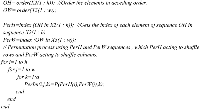
Step 6:

Convert the real sequence X3 to integer as $Z = fix\left( {X3_{i} \times {10}^{{{16}}} \bmod {256}} \right)$; then, perform Bit-XORed process on the sequence Z and the sequence of imaginary values Im of the Julia set to construct the second key sequence Key2 as $Key2 = Z \oplus {\text{Im}}$.

Step 7:

Substitute the permutated image (PerIm) using Key2 to obtain the final encrypted image (C). $C = PerIm \oplus Key2$.

Fig. 13

Visualization of the Julia set for c = − 0.745429

Fig. 14

Outline of the encryption process for the proposed encryption mechanism

7.2 Experimental analysis

With the aim to assess the proposed cryptosystem, experimentations are performed on a laptop equipped with Intel Core™ i7-3630QM, 16 GB RAM, and provided with MATLAB R2016b. Our dataset consists of three medical images each of size 256 × 256 (see Fig. 15) obtained from various medical image sources including the COVID-CT database [60] which is the most important database of COVID-19 computed tomography (CT) images available for the public. The initial values for iterating the presented HNN chaotic system are set as x₁₀ = 2, x₂₀ = 0, x₃₀ = 0, $\beta_{1} { = 0}{\text{.9,}}\,\,\,\beta_{2} { = 1}{\text{.15,}}\,\,\,\beta_{3} { = 1}{\text{.4}}$.

Fig. 15

Encryption issues and experimental dataset of images

7.2.1 Correlation of adjacent pixels

One of the fundamental tools to measure the robustness of an image is the correlation coefficient of adjacent pixels $C_{mn}$. For regular images, $C_{mn}$ values are near to 1 in every direction while for cipher images of a good encryption algorithm $C_{mn}$ values should close to 0 [59]. To evaluate $C_{mn}$, we randomly selected 10⁴ pairs of neighboring pixels in every direction. $C_{mn}$ are usually stated as follows:

$$ C_{mn} = \frac{{\sum\nolimits_{x = 1}^{A} {\left( {m_{x} - \overline{m}} \right)} \left( {n_{x} - \overline{n}} \right)}}{{\sqrt {\sum\nolimits_{x = 1}^{A} {\left( {m_{x} - \overline{m}} \right)^{2} \sum\nolimits_{x = 1}^{A} {\left( {n_{x} - \overline{n}} \right)^{2} } } } }} $$

(8)

where $m_{x}$, $n_{x}$ are used to point out the values of adjacent pixels and A points out the whole amount of nearby pixel pairs. It is evident from the outcomes plots presented in Fig. 16 that no profitable information can be retrieved from the encrypted data.

Fig. 16

Distribution of C_mn for original and cipher sample 1 image. This is the representation of pixels gray values on position (x + 1, y + 1) with respect to pixels gray values on position (x, y)

7.2.2 Information entropy

To assess the concentration of the pixel values in the image, information entropy is applied, which can be computed as:

$$ E(Y) = - \sum\limits_{a = 1}^{{2^{b} - 1}} {p(y_{a} } )\log_{2} \left( {p(y_{a} )} \right) $$

(9)

where $p(y_{a} )$ represents the possibility of $y_{a}$ and b indicates the pixel bit level, which is equivalent to the typical entropy value 8-bits [61]. Table 4 states the outcomes of entropy values for original images and their equivalent cipher ones, whose values for the cipher images are very close to 8.

Table 4 Outcomes of information entropy

7.2.3 Histogram test and Chi-square test

The reverberation of the organization of pixels in an image is evaluated using the histogram test. A good designed image encryption approach has a similar distribution of distinct cipher images for guaranteeing to resist statistical attacks [62]. Figure 17 presents the histograms of the experimented grayscale images which are distinct from each other, whereas the distributions of their equivalent cipher ones are identical with each other and are almost flat. This uniformity may be verified by using the Chi-square test. Table 5 provides the results of Chi-square values with 0.05 as weight value. Usually, the flatness of the histogram is validated if Chi-square value of the test sample is less than 293.2478 indicating a p value higher than 0.5. Regarding Table 5, the histogram test of various test samples is validated.

Fig. 17

Histograms of the experimented grayscale images for original and cipher images. This is the representation of frequency distribution of pixels with respect to their respective gray values

Table 5 Chi-square values for each encrypted test data

7.2.4 NPCR tests

The outcome of varying pixels in the original image on its equivalent cipher one is measured using NPCR (“Number of Pixels Change Rate”), which can be computed as follows.

$$ {\text{NPCR}}_{P,C} = \frac{{\sum\nolimits_{m;n} {{\text{Diff}}(m,n)} }}{D} \times 100\% ,\quad {\text{Diff}}(m,n) = \left\{ {\begin{array}{*{20}l} 0 \hfill & {{\text{if}}\,\,P(m,n) = C(m,n)} \hfill \\ 1 \hfill & {{\text{if}}\,\,P(m,n) \ne C(m,n)} \hfill \\ \end{array} } \right. $$

(10)

here D denotes the complete pixel numbers in the image. The outcomes of NPCR for the experimented dataset are displayed in Table 6, in which the medium value for the experimented dataset is 99.6175%; consequently, the given encryption approach is high sensitive to tiny pixel changes in the original image.

Table 6 Outcomes of NPCR test for the experimented dataset

7.2.5 Time analysis and comparison of the proposed cryptosystem

One of the important measures to assess the performance of an algorithm is its running speed. Definitely, an encryption algorithm should take minimum execution time so that it can be effectively used in enciphering images. Table 7 shows the running speed of Sample 1 images for different sizes. The computational platform is equipped with Intel^® core TM i7-3630QM 16 GB RAM and a MATLAB R2016b software. The computational time increases with respect to the size of the plain image. Note this computational time also relies on the capacity of the workstation (the processor and the RAM). Table 7 shows that an acceptable running speed is obtained and the algorithm is competitive with the results of the literature.

Table 7 Comparison of the running speed of sample 1 images

8 Comparative analyses and discussions

This analysis is done in two ways: First, we show the superiority of the dynamical behaviors on the proposed HNN. Second, we compare the results of the encryption scheme with the existing literature.

8.1 Dynamic analysis

Very recently, several research works have been carried out on the dynamic analysis of some particular classes of HNNs among with those with fixed activation gradients and those with variable activation gradients [12,13,14,15, 20, 38]. From some of these works summarized in Table 8, it has been found that the investigated models were the phenomenon of the multistability characterized by the coexistence of several firing patterns for the same set of the synaptic weights by starting from different initial conditions. The obtained results were further supported/validated using either hardware experiments of PSPICE simulations. It is well known that in some cases the multistable behavior is an undesirable behavior and needs to beavoid sometimes. This is why in this work, we introduce a simple 3D HNNs with variable activation gradient.

Table 8 Synthesis of some recent attractive works of the HNNs literature

In addition, we show the introduced model is able to display the coexistence of up to six disconnected firing patterns. We equally used the linear augmentation method to annihilate the coexisting pattern of the neural networks. It is good to mention that this annihilation process of the multistability has not yet been addressed in the previous works related to such neural networks with coexisting behavior as well as the application in engineering.

8.2 Encryption technics

A variety of encryption methods can be found in the literature and classified either as a spatial domain or frequency domain encryption algorithms. The first method directly considers the pixel of the original image without any transformation. The second method applies a mathematical transformation on the original image to compute some coefficients based on image pixels. Transform domain-based algorithms seem to be more efficient and robust than the spatial domain. In this paper, we will use the Julia set and the discrete sequences of the proposed HNN to transform the pixels of the plain image. Then, the controlled sequences of a simple 3D Hopfield neural network will be applied for encryption. Some achievements of the proposed encryption technics are resumed in Table 9, and a comparative analysis is carried out. It is obvious that the proposed encryption scheme provides high security over the existing literature.

Table 9 Comparative analysis for sample 1 data

9 Conclusion

In this paper, a novel simple 3D autonomous HNN has been introduced and investigated. Based on nonlinear analysis technics, we have demonstrated that the investigated system was able to exhibit the phenomenon of multistability with up to six competing attractors. Using the linear augmentation method, we have equally controlled the multistable found in the HNN for some suitable choice of controller parameters as well as the coupling strength. Remark that, in the work of [39], the surviving attractor was different from the initial coexisting ones, whereas in the control scheme adopted in this work, the surviving attractor is one among the initial coexisting attractors. It is found that the control goal is achieved for the highest of the coupling strength and the multistable HNN is metamorphosed in a monostable HNN. PSPICE simulations are also provided to support the obtained results. It is important to stress that the linear augmentation method has been considered in the literature only to control two or three different attractors (i.e., bistable or tri-stable systems) [39]. Also to the best of authors’ knowledge, no other chaotic system, particularly no HNN with up to six disconnected stable states, was successfully controlled in the literature until date. Thus, the present results contribute to enrich the literature about multistability and multistability control. Finally, a simple encryption scheme is designed jointly using the sequences of the proposed HNN and the sequences of real/imaginary values of the Julia fractals set. It is shown that the obtained cryptosystem is competitive with the results of the literature given that the proposed method achieved entropy of 7.9992, NPCR of 99.6299, and encryption time of 0.21 for the 256*256 sample 1 image. These results can be improved in the next future by exploring the effect of the adapting synapse-based neuron model also known as the tabu learning neuron model with their applications to secure medical images in IoHT.

References

Hopfield JJ (1984) Neurons with graded response have collective computational properties like those of two-state neurons. Proc Natl Acad Sci 81(10):3088–3092
Qiu H et al (2012) A fast ℓ1-solver and its applications to robust face recognition. J Ind Manag Optim (JIMO) 8:163–178
Wang Y et al (2010) An alternative Lagrange-dual based algorithm for sparse signal reconstruction. IEEE Trans Signal Process 59(4):1895–1901
Chanthorn P et al (2020a) A Delay-dividing approach to robust stability of uncertain stochastic complex-valued Hopfield delayed neural networks. Symmetry 12(5):683
Chanthorn P et al (2020b) Robust stability of complex-valued stochastic neural networks with time-varying delays and parameter uncertainties. Mathematics 8(5):742
Chanthorn P et al (2020c) Robust dissipativity analysis of hopfield-type complex-valued neural networks with time-varying delays and linear fractional uncertainties. Mathematics 8(4):595
Sriraman R et al (2020) Discrete-time stochastic quaternion-valued neural networks with time delays: an asymptotic stability analysis. Symmetry 12(6):936
Yang X-S, Yuan Q (2005) Chaos and transient chaos in simple Hopfield neural networks. Neurocomputing 69(1–3):232–241
Habutsu T et al (1991) A secret key cryptosystem by iterating a chaotic map. In Workshop on the theory and application of cryptographic techniques. Springer.
Biham E, Shamir A (1991) Differential cryptanalysis of DES-like cryptosystems. J Cryptol 4(1):3–72
Baptista M (1998) Cryptography with chaos. Phys Lett A 240(1–2):50–54
Bao B et al (2017a) Numerical analyses and experimental validations of coexisting multiple attractors in Hopfield neural network. Nonlinear Dyn 90(4):2359–2369
Njitacke Z, Kengne J (2018) Complex dynamics of a 4D Hopfield neural networks (HNNs) with a nonlinear synaptic weight: coexistence of multiple attractors and remerging Feigenbaum trees. AEU-Int J Electron Commun 93:242–252
Njitacke Z, Kengne J, Fotsin H (2019) A plethora of behaviors in a memristor based Hopfield neural networks (HNNs). Int J Dyn Control 7(1):36–52
Xu Q et al (2018) Two-neuron-based non-autonomous memristive Hopfield neural network: numerical analyses and hardware experiments. AEU-Int J Electron Commun 96:66–74
Cushing JM, Henson SM, Blackburn CC (2007) Multiple mixed-type attractors in a competition model. J Biol Dyn 1(4):347–362
Upadhyay RK (2003) Multiple attractors and crisis route to chaos in a model food-chain. Chaos Solitons Fractals 16(5):737–747
Njitacke Z et al (2020) Hysteretic dynamics, space magnetization and offset boosting in a third-order memristive system. Iran J Sci Technol Trans Electr Eng 44(1):413–429
Fonzin Fozin T et al (2019a) On the dynamics of a simplified canonical Chua’s oscillator with smooth hyperbolic sine nonlinearity: hyperchaos, multistability and multistability control. Chaos Interdiscip J Nonlinear Sci 29(11):113105
Tabekoueng Njitacke Z, Kengne J, Fotsin HB (2020) Coexistence of multiple stable states and bursting oscillations in a 4D Hopfield neural network. Circuits Syst Signal Process 39:3424–3444. https://doi.org/10.1007/s00034-019-01324-6
Tabekoueng Njitacke Z et al (2020) Coexistence of firing patterns and its control in two neurons coupled through an asymmetric electrical synapse. Chaos Interdiscip J Nonlinear Sci 30(2):023101
Tchinda T et al (2019) Dynamics of an optically injected diode laser subject to periodic perturbation: occurrence of a large number of attractors, bistability and metastable chaos. Sci J Circuits Syst Signal Process 8:66
Wouapi KM et al (2020) Various firing activities and finite-time synchronization of an improved Hindmarsh–Rose neuron model under electric field effect. Cogn Neurodyn 14:375–397
Wei Z et al (2015a) Study of hidden attractors, multiple limit cycles from Hopf bifurcation and boundedness of motion in the generalized hyperchaotic Rabinovich system. Nonlinear Dyn 82(1–2):131–141
Wei Z et al (2015b) Hidden attractors and dynamical behaviors in an extended Rikitake system. Int J Bifurc Chaos 25(02):1550028
Wei Z, Zhang W, Yao M (2015) On the periodic orbit bifurcating from one single non-hyperbolic equilibrium in a chaotic jerk system. Nonlinear Dyn 82(3):1251–1258
Bao B et al (2016a) Coexisting infinitely many attractors in active band-pass filter-based memristive circuit. Nonlinear Dyn 86(3):1711–1723
Bao B-C et al (2016b) Extreme multistability in a memristive circuit. Electron Lett 52(12):1008–1010
Njitacke Z, Kengne J, Negou AN (2017) Dynamical analysis and electronic circuit realization of an equilibrium free 3D chaotic system with a large number of coexisting attractors. Optik 130:356–364
Njitacke Z et al (2018) Uncertain destination dynamics of a novel memristive 4D autonomous system. Chaos Solitons Fractals 107:177–185
He S et al (2018) Multivariate multiscale complexity analysis of self-reproducing chaotic systems. Entropy 20(8):556
Sprott JC et al (2017) Megastability: coexistence of a countable infinity of nested attractors in a periodically-forced oscillator with spatially-periodic damping. Eur Phys J Spec Top 226(9):1979–1985
Tang Y et al (2018) Carpet oscillator: a new megastable nonlinear oscillator with infinite islands of self-excited and hidden attractors. Pramana 91(1):11
Leutcho GD et al (2020a) A new megastable nonlinear oscillator with infinite attractors. Chaos Solitons Fractals 134:109703
Leutcho GD et al (2020b) A new oscillator with mega-stability and its Hamilton energy: infinite coexisting hidden and self-excited attractors. Chaos Interdiscip J Nonlinear Sci 30(3):033112
Giakoumis A et al (2020) Analysis, synchronization and microcontroller implementation of a new quasiperiodically forced chaotic oscillator with megastability. Iran J Sci Technol Trans Electr Eng 44(1):31–45
Bao B et al (2017b) Coexisting behaviors of asymmetric attractors in hyperbolic-type memristor based Hopfield neural network. Front Comput Neurosci 11:81
Bao B et al (2019) Dynamical effects of neuron activation gradient on Hopfield neural network: numerical analyses and hardware experiments. Int J Bifurc Chaos 29(04):1930010
Canavier CC et al (1999) Control of multistability in ring circuits of oscillators. Biol Cybern 80(2):87–102
Pisarchik AN, Kuntsevich BF (2002) Control of multistability in a directly modulated diode laser. IEEE J Quantum Electron 38(12):1594–1598
Pecora LM, Carroll TL (1991) Pseudoperiodic driving: eliminating multiple domains of attraction using chaos. Phys Rev Lett 67(8):945
Chizhevsky V, Turovets S (1993) Small signal amplification and classical squeezing near period-doubling bifurcations in a modulated CO2-laser. Opt Commun 102(1–2):175–182
Pisarchik AN, Feudel U (2014) Control of multistability. Phys Rep 540(4):167–218
Pisarchik AN, Goswami BK (2000) Annihilation of one of the coexisting attractors in a bistable system. Phys Rev Lett 84(7):1423
Sharma PR et al (2014) Controlling dynamical behavior of drive-response system through linear augmentation. Eur Phys J Spec Top 223(8):1531–1539
Sharma P et al (2015) Control of multistability in hidden attractors. Eur Phys J Spec Top 224(8):1485–1491
Sharma PR et al (2011) Targeting fixed-point solutions in nonlinear oscillators through linear augmentation. Phys Rev E 83(6):067201
Fonzin Fozin T et al (2019b) Control of multistability in a self-excited memristive hyperchaotic oscillator. Int J Bifurc Chaos 29(09):1950119
Gao T, Chen Z (2008) A new image encryption algorithm based on hyper-chaos. Phys Lett A 372(4):394–400
Zhou Y, Cao W, Chen CP (2014) Image encryption using binary bitplane. Signal Process 100:197–207
Wang X-Y, Li Z-M (2019) A color image encryption algorithm based on Hopfield chaotic neural network. Opt Lasers Eng 115:107–118
Lakshmi C et al (2020) Hopfield attractor-trusted neural network: an attack-resistant image encryption. Neural Comput Appl 32(15):11477–11489
Kountchou M et al (2017) Optimisation of the synchronisation of a class of chaotic systems: combination of sliding mode and feedback control. Int J Nonlinear Dyn Control 1(1):51–77
Wouapi MK, Fotsin BH, Ngouonkadi EBM et al (2020) Complex bifurcation analysis and synchronization optimal control for Hindmarsh–Rose neuron model under magnetic flow effect. Cogn Neurodyn. https://doi.org/10.1007/s11571-020-09606-5
Shi K et al (2020a) Reliable asynchronous sampled-data filtering of T–S fuzzy uncertain delayed neural networks with stochastic switched topologies. Fuzzy Sets Syst 381:1–25
Shi K et al (2020b) Non-fragile memory filtering of TS fuzzy delayed neural networks based on switched fuzzy sampled-data control. Fuzzy Sets Syst 394:40–64
Shi K et al (2020c) Hybrid-driven finite-time H∞ sampling synchronization control for coupling memory complex networks with stochastic cyber attacks. Neurocomputing 387:241–254
Tsafack N et al (2020) Design and implementation of a simple dynamical 4-D chaotic circuit with applications in image encryption. Inf Sci 515:191–217
Rani M, Kumar V (2004) Superior Julia set. Res Math Educ 8(4):261–277
Yang X et al (2020) COVID-CT-dataset: a CT scan dataset about COVID-19. arXiv:2003.13865
Nestor T et al (2020) A multidimensional hyperjerk oscillator: dynamics analysis, analogue and embedded systems implementation, and its application as a cryptosystem. Sensors 20(1):83
Abd-El-Atty B, El-Latif AAA, Venegas-Andraca SE (2019) An encryption protocol for NEQR images based on one-particle quantum walks on a circle. Quantum Inf Process 18(9):272
Diaconu A-V (2016) Circular inter-intra pixels bit-level permutation and chaos-based image encryption. Inf Sci 355:314–327
Jithin K, Sankar S (2020) Colour image encryption algorithm combining, Arnold map, DNA sequence operation, and a Mandelbrot set. J Inf Secur Appl 50:102428
Liu L, Zhang Q, Wei X (2012) A RGB image encryption algorithm based on DNA encoding and chaos map. Comput Electr Eng 38(5):1240–1248
Author information
Authors and Affiliations
Corresponding author
Ethics declarations
Conflict of interest
The authors declare that they have no conflict of interest.
Additional information
Publisher's Note
Springer Nature remains neutral with regard to jurisdictional claims in published maps and institutional affiliations.
Rights and permissions
About this article
Cite this article
Njitacke, Z.T., Isaac, S.D., Nestor, T. et al. Window of multistability and its control in a simple 3D Hopfield neural network: application to biomedical image encryption. Neural Comput & Applic 33, 6733–6752 (2021). https://doi.org/10.1007/s00521-020-05451-z
Received:
Accepted:
Published:
Issue Date:
DOI: https://doi.org/10.1007/s00521-020-05451-z