Hybrid differential evolution and Nelder–Mead algorithm with re-optimization

Abstract

Nonlinear optimization algorithms could be divided into local exploitation methods such as Nelder–Mead (NM) algorithm and global exploration ones, such as differential evolution (DE). The former searches fast yet could be easily trapped by local optimum, whereas the latter possesses better convergence quality. This paper proposes hybrid differential evolution and NM algorithm with re-optimization, called as DE-NMR. At first a modified NM, called NMR is presented. It re-optimizes from the optimum point at the first time and thus being able to jump out of local optimum, exhibits better properties than NM. Then, NMR is combined with DE. To deal with equal constraints, adaptive penalty function method is adopted in DE-NMR, which relaxes equal constraints into unequal constrained functions with an adaptive relaxation parameter that varies with iteration. Benchmark optimization problems as well as engineering design problems are used to experiment the performance of DE-NMR, with the number of function evaluation times being employed as the main index of measuring convergence speed, and objective function values as the main index of optimum’s quality. Non-parametric tests are employed in comparing results with other global optimization algorithms. Results illustrate the fast convergence speed of DE-NMR.

Appendix

• 1. Weld beam design problem

  

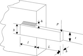  $$ \begin{aligned} {\text{Minimize}}\;& f\left( x \right) = 1.10471x_{1}^{2} x_{2} + 0.04811x_{3} x_{4} \left( {14 + x_{2} } \right) \\ {\text{subject}}\;to\;& g_{1} \left( x \right) = \tau \left( x \right) - 13,600 \le 0,\quad g_{2} \left( x \right) = \sigma \left( x \right) - 30,000 \le 0 \\ & g_{3} \left( x \right) = x_{1} - x_{4} \le 0,\quad g_{4} \left( x \right) = 0.1047x_{1}^{2} + 0.04811x_{3} x_{4} \left( {14.0 + x_{2} } \right) - 5.0 \le 0 \\ & g_{5} \left( x \right) = 0.125 - x_{1} \le 0,\quad g_{6} \left( x \right) = \delta \left( x \right) - 0.25 \le 0 \\ & g_{7} \left( x \right) = P - P_{c} \left( x \right) \le 0,\quad 0.1 \le x_{1} ,x_{4} \le 2 \\ & 0.1 \le x_{2} ,x_{3} \le 10 \\ \end{aligned} $$
  $$ \begin{gathered} \tau \left( x \right) = \sqrt {\left( {\tau^{\prime}} \right)^{2} + 2\tau^{\prime}\tau^{\prime\prime}{\frac{{x_{2} }}{{2{\text{R}}}}} + \left( {\tau^{\prime\prime}} \right)^{2} } ,\tau^{\prime} = {\frac{P}{{\sqrt 2 x_{1} x_{2} }}},\tau^{\prime\prime} = {\frac{QR}{J}},Q = P\left( {L + {\frac{{x_{2} }}{2}}} \right),R = \sqrt {{\frac{{x_{2}^{2} }}{4}} + \left( {{\frac{{x_{1} + x_{3} }}{2}}} \right)^{2} } \hfill \\ J = 2\left\{ {\sqrt 2 x_{1} x_{2} \left[ {{\frac{{x_{2}^{2} }}{12}} + \left( {{\frac{{x_{1} + x_{3} }}{2}}} \right)^{2} } \right]} \right\},\sigma \left( x \right) = {\frac{6PL}{{x_{4} x_{3}^{2} }}},\delta \left( x \right) = {\frac{{4PL^{3} }}{{Ex_{3}^{3} x_{4} }}},P_{c} \left( x \right) = {\frac{{4.013E\sqrt {x_{3}^{2} x_{4}^{6} } }}{{L^{2} }}}\left( {1 - {\frac{{x_{3} }}{2L}}\sqrt {{\frac{E}{4G}}} } \right) \hfill \\ P = 6,000,L = 14,E = 3 \times 10^{7} ,\quad G = 1.2 \times 10^{6} \hfill \\ \end{gathered} $$

• 2. Pressure vessel design problem

  

  $$ \begin{aligned} \min \;f &= 0.6224x_{1} x_{3} x_{4} + 1.7781x_{2} x_{3}^{2} + 3.1661x_{1}^{2} x_{4} + 19.84x_{1}^{2} x_{3} \\ {\text{s.t.}}\quad & g_{1} \left( x \right) = - x_{1} + 0.193x_{3} \le 0 \\ & g_{2} \left( x \right) = - x_{2} + 0.00954 \le 0 \\& g_{3} \left( x \right) = - \pi x_{3}^{2} x_{4} - {\frac{4}{3}}\pi x_{3}^{3} + 1,296,000 \le 0 \\ & 0 \le x_{1} ,x_{2} \le 100,10 \le x_{3} ,x_{4} \le 200 \\ \end{aligned} $$

• 3. Spring design problem

  $$ \begin{gathered} \min \;f = x_{1}^{2} x_{2} \left( {x_{3} + 2} \right) \hfill \\ {\text{s.t.}}\quad g_{1} \left( x \right) = 1 - {\frac{{x_{2}^{3} x_{3} }}{{71,785x_{1}^{4} }}} \le 0 \hfill \\ g_{2} \left( x \right) = {\frac{{4x_{2}^{2} - x_{1} x_{2} }}{{12,566\left( {x_{2} x_{1}^{3} - x_{1}^{4} } \right)}}} + {\frac{1}{{5,108x_{1}^{2} }}} - 1 \le 0 \hfill \\ g_{3} \left( x \right) = 1 - {\frac{{140.45x_{1} }}{{x_{2}^{2} x_{3} }}} \le 0 \hfill \\ g_{4} \left( x \right){\frac{{x_{1} + x_{2} }}{1.5}} - 1 \le 0 \hfill \\ 0.05 \le x_{1} \le 2,0.25 \le x_{2} \le 1.3,2 \le x_{3} \le 15 \hfill \\ \end{gathered} $$

• 4. Speed reducer design (gear train)

  $$ \begin{aligned} \min \;&f = 0.7854x_{1} x_{2}^{2} \left( {3.3333x_{3}^{2} + 14.9334x_{3} - 43.0934} \right) - 1.508x_{1} \left( {x_{6}^{2} + x_{7}^{2} } \right) \\ & \quad + 7.477\left( {x_{6}^{3} + x_{7}^{3} } \right) + 0.7854\left( {x_{4} x_{6}^{2} + x_{5} x_{7}^{2} } \right) \\ {\text{s.t.}}\quad & g_{1} \left( x \right) = {\frac{27}{{x_{1} x_{2}^{2} x_{3} }}} - 1 \le 0,\quad g_{2} \left( x \right) = {\frac{397.5}{{x_{1} x_{2}^{2} x_{3}^{2} }}} - 1 \le 0,\quad g_{3} \left( x \right) = {\frac{{1.93x_{4}^{3} }}{{x_{2} x_{3} x_{6}^{4} }}} - 1 \le 0, \\ & g_{4} \left( x \right) = {\frac{{1.93x_{5}^{3} }}{{x_{2} x_{3} x_{7}^{4} }}} - 1 \le 0 \\& g_{5} \left( x \right) = {\frac{{\sqrt {\left( {{\frac{{745x_{4} }}{{x_{2} x_{3} }}}} \right)^{2} + 16.9 \times 10^{6} } }}{{110x_{6}^{3} }}} - 1 \le 0, \\ & g_{6} \left( x \right) = {\frac{{\sqrt {\left( {{\frac{{745x_{5} }}{{x_{2} x_{3} }}}} \right)^{2} + 157.5 \times 10^{6} } }}{{85x_{7}^{3} }}} - 1 \le 0,\quad g_{7} \left( x \right) = {\frac{{x_{2} x_{3} }}{40}} - 1 \le 0,\; \\ & g_{8} \left( x \right) = {\frac{{5x_{2} }}{{x_{1} }}} - 1 \le 0,\quad g_{9} \left( x \right) = {\frac{{x_{1} }}{{12x_{2} }}} - 1 \le 0,\quad g_{10} \left( x \right) = {\frac{{1.5x_{6} + 1.9}}{{x_{4} }}} - 1 \le 0, \\ & g_{11} \left( x \right) = {\frac{{1.1x_{7} + 1.9}}{{x_{5} }}} - 1 \le 0 \\ & 2.6 \le x_{1} \le 3.6,\quad 0.7 \le x_{2} \le 0.8,\quad 17 \le x_{3} \le 28,\quad 7.3 \le x_{4} \le 8.3, \\ & 7.3 \le x_{5} \le 8.3,\quad 2.9 \le x_{6} \le 3.9,\quad 5.0 \le x_{7} \le 5.5 \\ \end{aligned} $$

References

Akhtar S, Tai K, Ray T (2002) A socio-behavioral simulation model for engineering design optimization. Eng Optim 34(4):341–354
Baulac MD, Defrance J, Jean P (2007) Optimization of multiple edge barriers with genetic algorithms coupled with a Nelder–Mead local search. J Sound Vib 300(1–2):71–87
Becerra RL, Coello Coello CA (2006) Cultured differential evolution for constrained optimization. Comput Methods Appl Mech Eng 195(33–36):4303–4322
Bhattacharjya R, Datta B (2005) Optimal management of coastal aquifers using linked simulation optimization approach. Water Resour Manag 19(3):295–320
Caponio A, Neri F, Terroni V (2009) Super-fit control adaptation in memetic differential evolution frameworks. Soft Comput 13(8–9):811–831
Coath G, Halgamuge SK (2003) A comparison of constraint-handling methods for the application of particle swarm optimization to constrained nonlinear optimization problems. In: Proceedings of the 2003 congress on evolutionary computation. IEEE Press, Canberra, pp 2419–2425
Coello Coello CA, Montes EM (2002) Constraint-handling in genetic algorithms through the use of dominance-based tournament selection. Adv Eng Inform 16(3):193–203
Fan SL, Zahara E (2007) A hybrid simplex search and particle swarm optimization for unconstrained optimization. Eur J Oper Res 181(2):527–548
García S, Molina D, Lozano M, Herrera F (2009) A study on the use of non-parametric tests for analyzing the evolutionary algorithms’ behaviour: a case study on the CEC’2005 special session on real parameter optimization. J Heuristics 15(6):617–644
Hedar AR, Masao F (2006) Derivative-free filter simulated annealing method for constrained continuous global optimization. J Glob Optim 35(4):521–549
Himmelblau DM (1972) Applied nonlinear programming. McGraw-Hill, USA
Kannan BK, Kramer SN (1994) An augmented Lagrange multiplier based method for mixed integer discrete continuous optimization and its applications to mechanical design. J Mech Des 116(2):318–320
Koziel S, Michalewicz Z (1999) Evolutionary algorithms, homomorphous mappings, and constrained parameter optimization. Evol Comput 7(1):19–44
Krasnogor N, Smith J (2005) A tutorial for competent memetic algorithms: Model, taxonomy, and design issues. IEEE Trans Evol Comput 9(5):474–488
McKinnon KIM (1995) Two strictly convex examples where the Nelder–Mead simplex method converges to a non-stationary point. Technical report, Department of Mathematics and Computer Science, University of Edinburgh, Edinburgh
Mezura-Montes E, Coello Coello CA (2005) A simple multimembered evolution strategy to solve constrained optimization problems. IEEE Trans Evol Comput 9(1):1–17
Pierret S, Coelho RF, Kato H (2007) Multidisciplinary and multiple operating points shape optimization of three-dimensional compressor blades. Struct Multidiscip Optim 33(1):61–70
Ray T, Liew KM (2003) Society and civilization: an optimization algorithm based on the simulation of social behavior. IEEE Trans Evol Comput 7(4):386–396
Suarez M, Tortosa P, Carrera J, Jaramillo A (2008) Pareto optimization in computational protein design with multiple objectives. J Comput Chem 29(16):2711–27041
Talbi E-G (2002) A taxonomy of hybrid metaheuristics. J Heuristics 8(5):541–564
Wang Y, Cai ZX, Zhou Y, Fan Z (2009) Constrained optimization based on hybrid evolutionary algorithm and adaptive constraint-handling technique. Struct Multidiscip Optim 37(4):395–413
Wei LY, Mei Z (2005) A niche hybrid genetic algorithm for global optimization of continuous multimodal functions. Appl Math Comput 160(3):649–661
Zahara E, Kao YT (2008) Hybrid Nelder–Mead simplex search and particle swarm optimization for constrained engineering design problems. Exp Syst Appl 36(2):3880–3886
Acknowledgment
Special thanks to the Francisco Herrera and anonymous editors for their valuable advices!
Author information
Authors and Affiliations
Corresponding author
Additional information
The work was supported by National 863 Hi-Tech Program #2006AA04Z160.