Are the Standard V_S-Kappa Host-to-Target Adjustments the Only Way to Get Consistent Hard-Rock Ground Motion Prediction?

Abstract

Site-specific seismic hazard studies involving detailed account of the site response require the prior estimate of the hazard at the local reference bedrock level. As the real characteristics of such local bedrock often correspond to “hard-rock” with S-wave velocity exceeding 1.5 km/s, “standard rock” PSHA estimates should be adjusted in order to replace the effects of “standard-rock” characteristics by those corresponding to the local bedrock. The current practice involves the computation of scaling factors determined on the basis of V_S (S-wave velocity) and “κ₀” (site specific, high-frequency attenuation parameter) values, and generally predicts larger high-frequency motion on hard rock compared to standard rock. However, it also proves to be affected by large uncertainties (Biro and Renault, Proceedings of the 15th world conference on earthquake engineering, 24–28, 2012; Al Atik et al., Bull Seism Soc Am 104(1):336–346 2014), mainly attributed to (i) the measurement of host and target parameters, and (ii) the forward and inverse conversions from the response spectrum domain to the Fourier domain to apply the V_S and κ₀ adjustments. Moreover, recent studies (Ktenidou and Abrahamson, Seismol Res Lett 87(6):1465–1478, 2016) question the appropriateness of current V_S− κ₀ scaling factors, so that the significant amplification of high frequency content for hard-rock with respect to standard-rock seems overestimated. This paper discusses the key aspects of a few, recently proposed, alternatives to the standard approach. The calibration of GMPEs directly in the Fourier domain rather than in the response spectrum domain is one possibility (Bora et al., Bull Seism Soc Am 105(4):2192–2218, 2015, Bull Earthq Eng 15(11):4531–4561, 2017). Another possibility is the derivation of GMPEs which be valid also for hard-rock conditions (e.g. Laurendeau et al., Bull Earthq Eng 16(6):2253–2284, 2018). In this latter case the host site response is first removed using theoretical site response analyses (and site velocity profile), or generalized inversions techniques. A third possibility is to use existing hard rock surface recordings to derive purely empirical scaling models from standard rock to hard rock (Ktenidou et al., PEER Report, Pacific Earthquake Engineering Research Center, Berkeley, 2016). Finally, when a sufficient amount of records are available at a given site, generic GMPEs can be scaled to the site-specific ground motion using empirical site residual (δ_S2Ss) (Kotha et al., Earthq Spectra 33(4):1433–1453, 2017; Ktenidou et al.,  Bulletin of Earthquake Engineering 16(6):2311–2336, 2018). Such alternative approaches present the advantage of a significant simplification with respect to the current practice (with thus a reduced number of uncertainty sources); their generalization calls however for high-quality recordings (including high-quality site metadata) for both host regions and target sites, especially for small to moderate magnitude events. Our answer to the question in the title is thus “No, alternative approaches exist and are promising; though, their routine implementation requires additional work regarding systematic site characterization (for the host regions) and high-quality site characterization/instrumentation (for the target site), and so do also the needed improvements of the existing HTTA procedure”.

1 Introduction

To account for the local site response within a seismic hazard assessment (SHA) study can be achieved following different approaches (e.g., Aristizábal, 2018). The simplest generic methods use Ground Motion Prediction Equations (GMPEs) where site conditions are characterized only by simple site proxies such as the average shear wave velocity over the upper 30 m, V_S30 (e.g. Bindi et al., 2017), soil classes based on site period (e.g., Zhao et al., 2016), or “depth to bedrock”. Such methods only return an average response from a large number of sites within the same class, but cannot capture the whole features of a specific site response and may be either over- or un-conservative. The most advanced, fully site-specific, methods explicitly account for the local site response and are preferable for the design of critical facilities, even though they are more complex and may have to cope with additional sources of uncertainties (Bazzurro and Cornell 2004a, b; Aristizábal et al., 2018). They need two fundamental elements: (i) an accurate estimation of the local site response, and (ii) a reliable estimate of the “reference” ground motion, i.e. the input motion at the specific bedrock beneath the considered site. The latter issue is the focus of the present paper.

In site-specific seismic hazard studies, it is thus common practice to first assess the ground motion at reference bedrock using GMPEs and then to perform site response analyses to obtain the free field ground motion at the considered site (Renault et al., 2013; Renault, 2014; Rodriguez-Marek et al., 2014; Ameri et al., 2017). Provided that the soil column lying above the reference bedrock is well described in terms of dynamic behaviour, this approach has the potential advantage of accounting for more realistic estimates of site response than when using generic GMPE site terms. Nevertheless, the characteristics of the bedrock beneath the considered site can significantly differ from those of the rock sites involved in the derivation of most GMPEs. The latter are most often— almost always indeed—representative of “standard” rock conditions with S-wave velocities around 800 m/s (e.g. Laurendeau et al., 2013) while the reference bedrock for the considered site often consists of “hard-rock” with a S-wave velocity much higher than 1 km/s. The standard practice (e.g., Campbell 2003; Al Atik et al., 2014) recommends performing “host-to-target” adjustments in order to remove the effects of the average “standard” rock characteristics of strong motion databases and to replace them by the effects of the bedrock characteristics of the considered site. These adjustments are presently based on differences in two parameters: the shear-wave velocity profile V_S and the “κ₀” parameter, considered to characterize the “site-specific” component of the high-frequency decay of ground motion (Anderson and Hough 1984; Silva and Darragh 1995; Campbell 2009). These adjustments are indeed an important source of uncertainty which significantly contributes to the global uncertainties of the SHA, as shown for instance in Biro and Renault (2012). These uncertainties are related to two main steps, which prove to be rather difficult to perform and are thus associated with large uncertainties: (i) the measurement of host and target parameters; (ii) the forward and inverse conversions from the response spectrum domain to the Fourier domain needed to apply the V_S and κ adjustments. Concerning the first one, and more especially the κ estimation, recent studies demonstrated a) that “first generation” V_S30-κ₀ relationships, often used to assess both host and target κ parameters, are not robust (e.g. Ktenidou et al., 2015; Edwards et al., 2015; Ktenidou and Abrahamson, 2016), and b) that the measurement of κ at the considered site may be significantly biased by high-frequency site amplifications (Parolai and Bindi, 2004; Perron et al., 2017), as well as by the specific setup of the corresponding seismological sensor (Hollender et al., 2018b). As indicated by Laurendeau et al. (2018) and again emphasized later in this paper, the consequence is that the increase of the high frequency content from standard-rock to hard-rock conditions, as provided by the present adjustment practice, does not seem to be relevant anymore.

Another important point that should be kept in mind is that the adjustment approach described above implicitly assumes that the ground motion predicted for the “standard-rock” by current GMPEs is an average one for the considered site proxy (i.e. V_S30), without any specific attention to local resonance effect related to lithological or morphological effects. The typical adjustment to a reference hard-rock condition then only concerns the effects related to differences in impedance contrast (through the V_S profile) and high-frequency attenuation between the host regions and the target site. However, it has recently been shown that “standard” rock is not totally exempt of resonant-type amplifications: Felicetta et al. (2018) show that about half of the rock sites in Italy (a typical host region for European ground motion) show non-negligible amplifications at variable frequencies, possibly due to the presence of weathered rock or thin soft layers above more consistent rock, with also potential interaction with surface topography effects, while Laurendeau et al. (2018) report similar conclusions for the KiK-net stations corresponding to stiff soil or rock sites. Using the ground motion estimated by the standard adjustment approach at reference bedrock as input for site-response analyses might therefore result in misestimating the site effects.

Alternative approaches to this practice have recently been proposed with the aim of both reducing the uncertainties mentioned above and avoiding to double-count site effects. The present paper intends to highlight the principle and the pros and cons of some of these alternative approaches. After a short overview of the present “V_S30- κ” adjustment practice, it will address successively the derivation and calibration of GMPEs directly in the Fourier domain rather than in the response spectrum domain (Bora et al., 2015, 2017), the direct derivation of GMPEs for hard-rock reference motion (e.g. Laurendeau et al., 2018), the derivation of combined V_S and κ empirical scaling factors for rock to hard-rock ground motion (Ktenidou and Abrahamson, 2016), and the use of site-specific, hard-rock residuals (δ_S2Ss), to correct the existing GMPEs (Kotha et al., 2017; Ktenidou et al., 2018), together with a few considerations about the potential use of physics-based models. The first approach (Bora et al., 2015, 2017) aims at removing the uncertainties associated to step (ii) described above, while still using the two site proxies V_S30 and κ. The second one (Laurendeau et al., 2018) is based on a characterization of rock sites through only the V_S30 velocity proxy (as almost all existing GMPEs), thus skipping all κ-related issues, and hence difficulties linked to steps (i) and (ii) mentioned above. Nevertheless this approach involves some assumptions and modeling to correct ground motion either from downhole (within motion) to surface (outcropping motion), or from site surface to outcropping hard-rock. The third approach (Ktenidou and Abrahamson, 2016) also allows to skip all κ-related issues by only using the V_S30 information, but still needs to be validated using broader hard rock datasets, representative of a larger variety of hard-rock conditions with actually measured site characteristics. The latter one (using δ_S2Ss residuals)—which could also be combined with the first two—does not need any site proxy—but requires a large enough number of local instrumental recordings. The conclusion section will highlight the various advantages of these alternative approaches, among which their simplicity with respect to the present practice.

2 Present State-of-the-Practice

The definition of the “reference” hard-rock ground motion is indeed a critical part of any fully site-specific seismic hazard study. This issue is faced in particular in the (relatively frequent) case of a facility located on a thick alluvial or sedimentary cover (a few tens to a few hundred meters): the amplification phenomena are controlled to the first order by the velocity contrast at the sediment/bedrock interface, and when the latter is deep enough for the bedrock to be un-weathered, its S-wave velocity can largely exceed 2000 m/s. Such a situation is encountered for instance in the ILL research neutron reactor in Grenoble and most of the Rhône Valley in France where the Messinian crisis led to deep indentation of the bedrock, now filled with sediments, or even in the Cadarache area characterized by relatively stiff soils overlying high velocity limestone (Garofalo et al., 2016; Hollender et al., 2018b).

The current GMPEs developed from surface recordings, are hardly constrained for hard-rock site conditions due to the lack of accelerometric stations installed on such geological conditions (even those on “standard rock” are not so frequent, and too often lack detailed geophysical characterization). The data used for developing presently available GMPEs are typically dominated by recordings at stiff soil and soft rock sites (e.g., V_S30 300- 700 m/s) (e.g., Laurendeau et al., 2013; Felicetta et al., 2018). Thus, predicted ground motion using GMPEs may not adequately represent the motion expected at the reference hard-rock. This requires adjusting the predictions obtained from GMPEs to account for the difference between the two rock references, i.e., “standard rock” and “hard-rock”.

2.1 V_S30-Kappa Adjustment

The current standard procedure to adjust the ground motion predicted for “standard-rock” to “hard-rock” conditions has received the name of “host-to-target adjustment” (HTTA in the following). It has been applied for example for the re-evaluation of seismic hazard for Swiss nuclear power plants (PEGASOS and PRP projects: Biro and Renault, 2012; Renault et al., 2013), for the “Thyspunt Nuclear Siting’ project in South Africa (Rodriguez-Marek et al., 2014), or for the Hanford site in the U.S. (Coppersmith et al., 2014).

The basic principle (Campbell, 2003; Cotton et al., 2006; Al Atik et al., 2014) is to (try to) take into account any possible differences in source, propagation, and site conditions between the host region and the target site using physics-based models. These adjustments thus require, in principle, a good understanding of the physical phenomena controlling ground motion, as well as a well-defined procedure for adjusting the corresponding GMPE terms or the resulting hazard values. However, the adjustments for the source (e.g., stress drop) and crustal propagation terms (e.g., quality factor, Moho depth) are generally not applied because the underlying physical phenomena are often poorly constrained in both “host” and “target” regions. Then, the adjustment factor applied in the current practice is typically based only on two types of corrections, one representative of the difference in impedance effects, related to differences in the V_S profiles between the “host” regions and the “target” site (V_S adjustment), and another one representative of differences in the attenuation at shallow depth, characterized by the high-frequency decay parameter κ₀ (κ adjustment). The present standard HTTA procedure is thus called V_S-κ adjustment. In short, the physics-based adjustments are made in the Fourier domain and transposed in the traditional domain of response spectra via random vibration theory (Campbell, 2003; Al Atik et al., 2014). The two correction factors are detailed in the following:

• The V_S adjustment factor corresponds to the crustal amplification factor, and is based on the impedance effects modeled by the “quarter-wavelength” approach (QWL in the following) initially proposed by Joyner et al. (1981). As shown by Boore (2003), the crustal amplification estimate is derived from the S-wave velocity profile down to the very deep bedrock, and exhibits a smooth and monotonic increase with frequency, with a maximum high frequency value of the order of the square root of the ratio (V_{S_surface}/V_{S_deepbedrock}). This approach neglects resonance effects related to possible superficial or deep contrasts (Boore, 2013). Moreover, its application requires the knowledge of the “average” velocity profile (down to several kms depth) of both the host region and target site. As the former is most often unknown in practice—if not the latter—, the workaround strategy is to use a family of “standard profiles” that are anchored on the available, shallow velocity values (V_S30, cf. Boore and Joyner 1997, Cotton et al. 2006, and Boore, 2016). This situation should however improve in the future, as several authors have proposed methods to derive specific reference rock profiles adapted to the considered region (e.g., Poggi et al., 2011 for Switzerland and Poggi et al., 2013 for Japan).

• The κ adjustment is related to the difference in the site-specific attenuation (characterized by the high-frequency decay parameter κ₀) between the host region and the target site, and introduces a modulation of the high frequency content: if the target site attenuates less than the rocky sites of the host region (κ_{0_target} < κ_{0_host}), the high frequency content of ground motion at target hard rock is increased. It has indeed been commonly accepted over the last two decades that the parameter κ₀ decreases when stiffness increases (e.g., Anderson and Hough, 1984; Hough et al., 1988).

The combined effect of impedance (QWL) and attenuation κ₀ thus generally leads to a slight decrease in low frequency motion (impedance effect), and a high frequency increase (attenuation effect), for “hard” rock compared to “standard” rock. The latter result, though accepted in the engineering community over the last two decades, is however considered counterintuitive by some seismologists, and is worth a careful analysis and discussion.

2.2 Practical Limitations

Applying such a HTTA procedure requires the knowledge of V_S30 and κ₀ values (and of the associated uncertainties) for the host region, and their measurements for the target site. While we reasonably dispose of measured V_S30 in “host” regions, measuring κ₀ is very delicate since it requires numerous enough, high-quality, on site instrumental recordings, and careful processing. For the target site, while one might dispose of a good quality V_S profile and V_S30 estimate, the measure of κ₀ presents still an additional issue which is that even instrumented sites seldom dispose of instruments located at the reference bedrock. Moreover, the standard adjustment practices as proposed by Al Atik et al. (2014) prove to be rather cumbersome and sometimes subjective. This HTTA approach is thus affected by a rather high level of epistemic uncertainty related to several factors, as detailed below, which may strongly impact the hazard and risk estimates, especially at long return periods. These uncertainties are of four types: the first one is related to the physics behind the so-called “κ₀” parameter, the second one is associated with the assessment of the host region parameters, the third one with the measurement of the target site parameter, and the last one is a methodological one related to the mathematical derivation of the adjustment factor.

• The physics underlying the use of the κ₀ parameters is assumed to be the attenuation features beneath the studied site (although a few authors also include some source related effects, e.g. Hassani and Atkinson, 2018). Low attenuation (assumed to be associated to hard rock) results in a rich high frequency content and a low κ₀ parameter. Indeed it is a fact that rigid sites statistically produce recordings with higher amount of high frequency content. However, this feature can be explained not only by a “lack” of attenuation (the only invoked phenomenon within the usual κ₀ interpretation), but also by local amplifications generated by less rigid, thin surface layers that cause high-frequency resonance (Parolai and Bindi, 2004; Laurendeau et al., 2018). The latter phenomenon is actually very common for free-field “rock” stations because of the presence of weathered layers (e.g., Cadet et al., 2010; Laurendeau et al., 2018). Figure 1 shows example amplifications for three RAP (French permanent accelerometric network) sites, PYLI, OGAN and OGCH, having measured V_S30 values of 1257 m/s, 1003 m/s and 1454 m/s, respectively (with a ± 15–20% uncertainty, Hollender et al., 2018a). The significant high frequency amplifications are due to local, shallow, weathered layers. This feature questions the accuracy and representativeness of κ measures for such situations that are very common in strong motion databases. There are also other phenomena that may modify the high frequency content of recordings, and therefore bias the κ₀ estimate and its interpretation as an attenuation parameter only, such as the choice of instrumental setup or the depth at which the sensor is installed, as illustrated in Hollender et al. (2018b). In addition, the link between κ₀ and attenuation also faces the issue of similar high-frequency effects due to scattering by near-surface heterogeneities, which can lead to measurement bias and/or misinterpretations, as shown by Ktenidou et al. (2015), Cabas et al. (2017), Pilz and Fäh (2017), and Shible et al. (2018).

  Fig. 1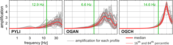

  

  From Hollender et al. (2018a)

  Example of 1D transfer functions computed using the V_S profiles inferred from surface-wave inversion for three RAP (French permanent accelerometric network) rock sites. For each station, 33 1D transfer functions were computed using 33 different V_S profiles to account for V_S profile uncertainties (grey lines), as well as their mean and standard deviation (red lines). All stations exhibit high-frequency amplification due to shallow weathered layers. The frequency identified by the green vertical line is the one above which amplification > 1.5.

• In general, on the “host” side, the S-wave velocity profile (involving not only V_S30, but also its shape down to several kilometers depth) and κ₀ are, at best, poorly known, and, in general, not constrained at all. It leads to the use of generic velocity profiles (Boore and Joyner, 1997; Cotton et al., 2006; Boore, 2016), while κ₀ values are derived either from V_S30-κ₀ statistical correlations, such as those proposed by Silva et al. (1998), Chandler et al. (2006), Douglas et al. (2010), Drouet et al. (2010), Edwards et al. (2011), Van Houtte et al. (2011), Cabas et al. (2017) and Kottke (2017), or from indirect estimates on Fourier spectra derived from response spectra using Inverse Random Vibration Theory (IRVT, Al Atik et al., 2014). The latter are hampered by the rather loose link between the high-frequency parts of Fourier and response spectra (Bora et al., 2016; Montejo and Vidot-Vega, 2018), while the analysis of the quoted V_S30-κ₀ correlations reveals a large variability in average trends from one study to another, as well as a huge dispersion of raw data leading to huge uncertainties associated to κ₀ estimates, especially for large V_S30 values. Recent studies indicate that the hard-rock κ₀ values (typically 0.006 s) proposed in the late 90’s - 2000’s for central-eastern United States on the basis of very few data and hastened estimates, could be affected by significant biases or measurement problems. In particular, Ktenidou and Abrahamson (2016) analyzed a set of records corresponding to sites with (inferred) V_S30 ≥ 1500 m/s (especially in the Eastern United States) for which reliable κ₀ measurements could be performed: they report both significantly higher κ₀ values (around 0.02 s) than expected from the usual correlations, and observed hard rock motion comparable to, or smaller than standard rock motion, over the entire frequency range, including high frequency.

• On the target side, even if the same type of “correlation” approach as for the host region can be used when there is no site-specific κ₀ measurement, it seems highly preferable (and consistent with a site-specific study) to determine truly site-specific values from an ad-hoc instrumentation, allowing the velocity profile and the κ₀ value to be much more precisely constrained. This was for instance the case for the Hanford site (Coppersmith et al., 2014), where the target κ₀ value could be constrained from a local array of stations along with generalized inversion techniques, and some a priori assumptions regarding the crustal attenuation (Silva and Darragh, 2014). This is relatively easy for outcropping hard-rock sites, but may be more difficult or expensive if there is no nearby hard-rock outcrop. Even for the outcropping rock case, the measurement can still be affected by several biases, as illustrated in Fig. 1 and Parolai and Bindi (2004), which can explain the dispersion of V_S30-κ₀ correlations, depending on the care taken to measure κ₀.

• Finally, two main sources of methodological uncertainties can be identified in the current HTTA approaches. First, the use of the impedance-only approach (or “quarter wave length” - QWL) to estimate the amplification functions related to the rock velocity profiles, neglects the effects of resonance (Boore, 2013) and therefore cannot account for high-frequency amplification peaks at many rocky sites (Steidl et al., 1996; Cadet et al., 2010). Then, the necessary back-and-forth conversions between the two spectral domains (Fourier and response spectra) via random vibration theory (RVT and IRVT, see Al Atik et al., 2014, Bora et al., 2015), introduce uncertainties because this process is highly nonlinear and non-unique, especially in the high-frequency range (Bora et al., 2016). It can be noted that most of these uncertainties come from the lack of knowledge of the rock velocity profiles and of the exact values of κ₀ for the host regions.

3 Alternative Approaches

3.1 Fourier Domain GMPEs

A first alternative approach that removes the variability associated with the back-and-forth conversions between response and Fourier spectral domains, is to work primarily in the Fourier domain. This may be done in two ways:

• Using generalized inversion techniques to identify in the Fourier domain the respective contributions of the source, path and site terms to the recorded ground motion. This needs a priori models such as the Brune model for the source (characterized by its moment M₀ and stress-drop Δσ), a given, parametric geometrical spreading functional form G(R), an anelastic attenuation term (“κ”), combining the crustal (Q) and site (“κ₀”) contributions, and a frequency-dependent site term. Such an approach, which is closely related with forward stochastic modelling using point sources as proposed by Boore (1983), has been implemented with the present scope in Bora et al. (2015, 2017), following a long list of studies using generalized inversion studies aiming at retrieving source, path or site terms (e.g., Drouet et al. 2008, 2010; Edwards and Fäh, 2013; Oth et al., 2011).

• Deriving “GMPEs” for Fourier spectra in the same way as for oscillator response spectra, i.e., in a purely empirical way where a priori functional forms with unknown coefficients are driven by the underlying physics (Bora et al., 2015).

Nevertheless, both approaches still involve one conversion from Fourier to response spectra (the less problematic one), which is performed using forward RVT and assumptions or empirical models about duration (Bora et al., 2015).

Such approaches offer the advantages of a) providing a way to estimate directly the “host” κ₀ value in a somehow physical—though indirect—way, and b) allowing an easy correction of crustal amplification and attenuation terms directly in the Fourier domain. For instance, the recent application to the European RESORCE data set (Bora et al., 2017) led to κ₀ values for nearly one hundred stations (Fig. 2), with several interesting observations: a large event-to-event variability for a given site, the absence of obvious correlation between κ₀ values and either V_S30, or site class, the class-to-class changes remaining much smaller than the event-to-event variability at a single site.

Fig. 2

κ₀ estimates obtained for European stations located on stiff sites (V_S30 ≥ 400 m/s) and having more than 10 recordings, plotted as a function of the corresponding V_S30 values. On the left, only small distance recordings are used (R ≤ 50 km), while the right plot accounts for all recordings for each station. Markers (empty circles, disks and empty squares indicate the median, while vertical bars indicate the range of 16-to-84 percentile of each station, i.e., the event-to-event variability. The horizontal solid line indicates the median value of all stations, while the two dashed lines indicate the corresponding 16 and 84 percentiles of all station median values, i.e., the between-station variability (similar to Bora et al., 2017)

There still exist however several limitations which hamper the generalization of such results:

• The very small number of rock stations with actually measured V_S30 values (Table 1) not only within the RESORCE data, but also within all presently existing strong motion data sets.

  Table 1 Site class median κ₀ values together with the 16–84% percentile range for Italy, Turkey and other European areas, together with the estimates of average, frequency independent crustal quality factors from Bora et al., 2017

• The simplicity of the point source models used in generalized inversion techniques, which are too poor to capture the behaviour of ground motion complexity in the near source area of large magnitude events, which often control the hazard. The next generation of generalized inversion techniques might include extended fault, which will however increase the number of source parameters, and the possibility of trade-off with other terms in case of too limited data set.

• The significant trade-off between the geometrical spreading term G(R), the crustal attenuation term (Q₀—with or without frequency dependence) and the site-specific attenuation term (κ₀), as illustrated in Fig. 3, so that those approaches cannot provide an “absolute” estimate of the site κ₀ value. The set of obtained values for G(R), Q₀(f) and κ₀, can however be used together in forward modelling. So that HTTA remain possible though requiring much care about the consistency of the three terms.

  Fig. 3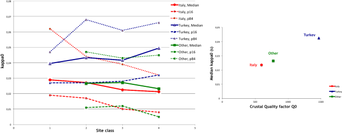

  

  Variability of the site-class specific κ₀ values derived from the RESORCE data base (Bora et al., 2017). Left: variation of κ₀ values with site class [from soft soil (“1”) to rock (“4”)] for Italy (red), Turkey (blue) and Other European areas (green). Solid line = median values, dashed line = 16% percentile, dotted line = 84% percentile. Right = variation of median regional κ₀ values with the inverted average, frequency independent quality factor

• The use of a “generic” crustal velocity profile imported from elsewhere (e.g., California) to estimate the “reference rock” crustal amplification, together with the use of the quarter wave-length approach to estimate the associated amplification, which thus leads to neglect possible high-frequency resonance effects and may induce some bias in κ₀ estimates.

For the generalization of such approaches, large number of recordings at rock stations are required. Also, more sensitive instruments are needed to increase the number of records for each station, in order to enable the reduction of the event-to-event variability in κ₀ estimates at a site.

3.2 Hard-Rock GMPEs

Another possibility consists of avoiding all κ₀ related issues by directly developing GMPEs for hard-rock motion, which be related only to the rock stiffness, i.e., the V_S30 value, in the same way most presently existing GMPEs rely only on V_S30 for predicting the ground motion on soft soils. Such GMPEs could then be applied without adjustment to the bedrock characteristics beneath the target site with large V_S. At present, the only available rock recordings which combine a large enough number with reliable, measured site metadata, are the deep sensor recordings of the KiK-net network. This direction was first explored by Cotton et al. (2008) and Rodriguez-Marek et al. (2011) who proposed GMPEs calibrated upon recordings obtained from these deep sensors. Their models are however not used in SHA studies because of the reluctance of many scientists or engineers to use depth recordings that are contaminated by a “within motion” effect (Bard and Tucker, 1985; Steidl et al. 1996), and are therefore smaller than outcropping motion—even with the same rock velocity.

An approach recently explored was thus to simply correct the deep sensor recordings using the depth-correction function proposed by Cadet et al. (2012a), in order to derive consistent outcrop motion. In short, the within-motion modulation induced at depth by interferences between up-going and surface-reflected down-going waves, is characterized, in the Fourier domain, by a maximum reduction (a spectral trough) at a destructive frequency, f_dest, controlled by the depth, Z, of the sensor, and the average speed, V_SZ, between the surface and the sensor (f_dest = V_SZ/4Z), possibly with smaller reductions at higher harmonics. At low frequency (f ≪ f_dest), the wavelength is much greater than the depth of the sensor, and the motion at depth is therefore identical to the outcropping surface motion; while at high frequencies (f ≫ f_dest), the interference effect leads to an average decrease close to a factor of 2, corresponding to the free surface effect. Cadet et al. (2012a) proposed a depth correction function to be applied on the response spectra, therefore corresponding to a smoothed version of the Fourier domain modulation: the surface/depth ratio (outcrop/within motion) varies from 1 at low frequency to a maximum of about 2.5 for f = f_dest, stabilizing around 1.8 for f > 5 f_dest, according to the following expression:

$$\begin{aligned} DCF\left( f \right) &= C_{1} \left( f \right) \times C_{2} \left( f \right), \hfill \\ \text{with}\, C_{1} \left( f \right) &= 1. + 1.6 \frac{{a\tan \left( {f/f_{dest} } \right)}}{\pi }\, \text{and}\, C_{2} \left( f \right) = 1 + 0.8e^{{ - \left\{ {\left( {{\raise0.7ex\hbox{$f$} \!\mathord{\left/ {\vphantom {f {f_{dest} }}}\right.\kern-0pt} \!\lower0.7ex\hbox{${f_{dest} }$}} - 1} \right)^{2} /0.09} \right\} }} . \hfill \\ \end{aligned}$$

(1)

In this expression, C₁(f) corrects for the free surface doubling effect, while C₂(f) corrects for the destructive interference effects at depth. Even though the latter correction should in theory include a modulation as a function of the impedance contrast when considered in the Fourier domain (i.e., the larger the impedance contrast, the smaller the peak width), Cadet et al., (2012a) preferred to omit this dependence for simplicity purposes, considering that this correction is applied to damped response spectra instead of Fourier spectra, and that the main issue is the correction for destructive interferences at depth, which occurs both in homogeneous and layered half-spaces, and is controlled by the average velocity between surface and the considered depth.

Laurendeau et al. (2018) applied this depth correction factor to the deep KiK-net recordings to generate a new dataset characterizing outcrop hard-rock motions (called “DHcor”). This was possible as its application only requires the knowledge of the value of the fundamental frequency of destructive interference f_dest, which can be obtained in two different ways: from the (known) velocity profile, V_S(z), between 0 and Z, and also from the average horizontal-to-vertical (H/V) spectral ratio of deep recordings (which exhibits a trough around f_dest). The two approaches are possible for deep KiK-net recordings, and have been found to produce comparable estimates of f_dest (Cadet et al., 2012b).

Nevertheless, as the availability of recordings at depth, together with corresponding hard-rock velocity measurements, is exceptional, Laurendeau et al. (2018) explored another approach which can be applicable to surface data from other networks. It consists of taking advantage of the knowledge of the velocity profile between 0 and Z to deconvolve the surface motion of the corresponding theoretical 1D transfer function, calculated with the reflectivity method of Kennett (1974) for vertically incident S-waves. In addition to a strong implicit assumption of only 1D surface effects, this approach also requires additional assumptions about the profile, specially regarding the quality factor—or attenuation—profile. In the absence of direct measurements, the current approximation of proportionality Q_S (z) = V_S (z)/X_Q with X_Q = 10 was selected, but a sensitivity study was conducted using X_Q values ranging from 5 to 50. Moreover, the 1D hypothesis was tested by comparing the simulated transfer functions with direct observations (surface/depth ratios), and retaining only the sites for which this comparison is satisfactory according to the correlation criteria proposed by Thompson et al. (2012). Here again, a sensitivity study was conducted to evaluate the robustness of the results with regard to the correlation threshold retained for the selection of 1D sites. As detailed in Laurendeau et al. (2018), both sensitivity studies concluded at a very satisfactory robustness of the median estimates of outcropping rock motion, and thus this deconvolution approach was applied to KiK-net surface recordings to generate another set, called “SURFcor”, of virtual hard-rock outcropping motion.

These two approaches have been applied by Laurendeau et al. (2018) to a subset of KiK-net data consisting of recordings obtained between 1999 and 2009 on stiff sites with V_S30 ≥ 500 m/s and depth velocity (V_SDH) ≥ 1000 m/s, and corresponding to crustal earthquakes with magnitudes ≥ 4.5 and hypocentral depth ≤ 25 km. It resulted in the constitution of two independent estimates of hard-rock ground motion (DHcor and SURFcor), for which the distribution in terms of V_SDH is almost uniform between 1000 and 3000 m/s (see Laurendeau et al., 2018 for further details about the data set).

It is then possible to derive GMPEs according to the standard procedures in order to quantify the dependence of ground motion on rock stiffness using the “c₁” site coefficient in the following, simple, GMPE functional form:

$$\begin{aligned} { \ln }\left( {{\text{SA}}\left( {\text{T}} \right)} \right)_{\text{es}} & = {\text{a}}_{ 1} \left( {\text{T}} \right) + {\text{a}}_{ 2} \left( {\text{T}} \right).{\text{ M}}_{\text{W}} + {\text{a}}_{ 3} \left( {\text{T}} \right).{\text{ M}}_{\text{W}}^{ 2} + {\text{b}}_{ 1} \left( {\text{T}} \right).{\text{ R}}_{\text{RUP}} \\ & \quad - { \ln }\left( {{\text{R}}_{\text{RUP}} } \right) + {\text{c}}_{ 1} \left( {\text{T}} \right). { \ln }\left( {{\text{V}}_{\text{S}} / 1000} \right) + \delta {\text{B}}_{\text{e}} \left( {\text{T}} \right) + \delta {\text{W}}_{\text{es}} \left( {\text{T}} \right), \\ \end{aligned}$$

where SA(T) is the spectral acceleration for the oscillator period T, M_w is the moment magnitude, R_RUP the distance to rupture, V_S the rock velocity (V_S30 at surface or V_SDH for corrected surface or down-hole recordings, i.e., the velocity of the sensor at depth), and δB_e and δW_es are the between- and within-event residuals, respectively.

Such relationships offer the advantage of not requiring any other site characteristic than the V_S value; in other words, any possible correlation between V_S and κ₀ is “hidden” behind the V_S dependence, but implicitly accounted for in average.

In order to analyze the robustness of the corresponding ground motion estimates, such GMPEs have been calibrated for several datasets:

• The original set of surface recordings (DATA_surf) and deep recordings (DATA_dh), the validity range of which correspond to 500-1000 m/s and 1000-3000 m/s, respectively.

• the corrected estimates SURFcor and DHcor (whose range of validity spans the range of downhole velocities, i.e. 1000-3000 m/s).

• Hybrid sets combining these last two sets with DATA_surf (whose validity range in V_S thus extends from 500 to 3000 m/s).

As detailed in Laurendeau et al. (2018), a similar average response spectrum prediction was obtained for sites characterized by high velocities (1000-3000 m/s) with the two different independent approaches (i.e., DHcor and SURFcor), and the hybrid sets as well: Whatever the initial data set and the correction procedure, the predictions indicate that the impedance effect is dominant at high frequency, with reduction factors 2 to 3 compared to the standard rock for frequencies above 8 Hz.

As a consequence, the main result in terms of adjustment factor is summarized in Fig. 4, which compares the ratio between the estimates on standard rock motion (V_S30 = 800 m/s), and on a “very hard” rock (V_S30 ≈ V_SDH = 2400 m/s) for the HTTA approach, as implemented in a traditional way with the V_S30-κ₀ relationships from Van Houtte et al. (2011), with those obtained with the alternative approaches discussed in the present section. It exhibits a good agreement at low frequency until about 2–3 Hz, where the impedance effect results in a slight (20–30%) decrease for hard-rock, and a strong disagreement at high frequency (beyond 5 Hz).

Fig. 4

Comparison of the hard-rock-to-rock adjustment factors obtained in different ways: (1) the theoretical one published by Van Houtte et al. (2011) using V_S30-κ₀ correlation; (2) the empirical models proposed by Ktenidou and Abrahamson (2016); (3) the ones obtained from the GMPEs developed by Laurendeau et al. (2018) using hybrid sets. The specific scenario considered here is: M_W = 6.5; R_RUP = 20 km

• The average correlation between V_S30 and κ₀ used in Van Houtte et al. (2011) leads to κ₀ values around 0.008 s for hard-rock, so that the effects of very small attenuation dominate those of higher impedance at high frequency: The HTTA approach using Van Houtte et al. (2011) thus predicts a larger hard-rock motion (compared to standard rock) beyond 7–8 Hz, with an amplification up to a factor 2 at 20–30 Hz.

• All other estimates obtained by Laurendeau et al. (2018), whatever the initial data set and the correction procedure, indicate that the impedance effect dominates over the whole frequency range, and especially at high frequency, with reduction factors about 2 to 3 compared to the standard rock for frequencies above 8 Hz.

The resulting difference between hard-rock motion predictions thus reaches a ratio about 4 at high frequency between a classical HTTA approach involving the usual V_S30- κ₀ correlations (as the one from Van Houtte et al., 2011), and alternative approaches based on hard-rock GMPEs built from KiK-net data. The magnitude of these high frequency differences obviously depends on the rock stiffness: they become negligible for rocks having S-wave velocities below 1200 m/s, but are even larger for very hard rock such as the one present underneath the Grenoble basin, with V_S close to 2800 m/s.

The robustness of the median results obtained with the two correction approaches (hybrid datasets based on SURFcor and DHcor, see Fig. 4) supports the questions about bias in the HTTA approach, and their possible origin as discussed above in Sect. 2.2. As stated in the discussion section of Laurendeau et al. (2018), this bias can be explained mainly by:

• an underestimation, of the high-frequency host site amplifications actually observed at the surface of KiK-net sites, which may be at least partly due to the use of generic velocity profiles, and of the QWL approach neglecting resonance effects, which both lead to an overestimation of the adjustment factor;

• an overestimation of the κ₀ effects due to strong bias in their measurement in relation with the frequency range of the high frequency rock amplification: κ₀ values are likely to be overestimated for “standard” rock conditions (measurement of κ in a frequency band beyond the peak amplification, i.e. beyond 5-10 Hz), and underestimated on “hard” rock sites exhibiting a similar resonance but at higher frequency, so that κ is measured in the frequency band below the amplification peak. This interpretation is supported by the latest, higher quality κ₀ measurements on hard-rock sites by Ktenidou and Abrahamson (2016) and Perron et al. (2017).

3.3 Empirical Scaling Models from Standard- to Hard-Rock

Recently, Ktenidou and Abrahamson (2016) used two hard-rock datasets (NGA-East and BCHydro) to develop an empirical scaling model for hard-rock with respect to standard-rock ground motion, which accounts for the combined effect of the V_S profile and of κ₀. This approach relies on a similar basic idea as the previous one, but from a purely empirical point of view.

The records from the two dataset are used up to 50 km, in order to minimize the effect of path attenuation. Figure 4 shows the scaling models proposed by these authors: Model 1 is based on BCHydro data, with average V_S30 around 2400 m/s, while Model 2 is based on NGA-East data, with average V_S30 estimated around 2000 m/s.

With respect to the previous approach, the hard-rock to standard-rock ground motion ratios obtained by Ktenidou and Abrahamson (2016) are closer to unity than those obtained here with the hybrid sets (Fig. 4) especially at high frequency. However, the datasets used by Ktenidou and Abrahamson (2016) to derive these ratios are relatively small, and they actually lack of measured V_S30 values for most of the hard-rock sites they considered (most of them were simply inferred).

Unambiguous answer to what the most appropriate model is, will undoubtedly come from large, high quality rock recordings for which both V_S30 and κ₀ values are carefully measured.

3.4 Site-Specific Residuals

The idea, which is implemented for instance in Kotha et al. (2017), is simply to take advantage of the recordings available at a given site to evaluate, for each GMPE of interest, the site-specific residual term δ_S2S(T) (average of δW_es(T) over all recordings) so as to tune each of them to the specific site under study. An example is given for instance in Ktenidou et al. (2018) for the Euroseistest site, from which Fig. 5 is taken.

Fig. 5

Period-dependence of site term residuals δ_S2Ss (T) (right) and of the associated variability φ_SS,s (T) (left) for four recording sites of the Euroseistest array. PRO is an outcropping rock site with a V_S30 around 600 m/s, PRO33 and TST196 are down-hole rock sites with V_S around 1400 and 1900 m/s, respectively, while TST is a surface, soft site (V_S30 = 186 m/s). The solid line corresponds to the case where no site term is included in the GMPE, while the dashed line corresponds to the case where the GMPE includes a site term related to the site proxy V_S30. From Ktenidou et al. (2018)

This approach is very appealing, as it combines the site-specificity from the available local recordings and the robustness of GMPEs derived on much larger and diverse data sets, and it should definitely be encouraged whenever possible. It should however be emphasized that such a local–global combination is possible if and only if a) the available local recordings have a good enough quality to offer an acceptable signal-to-noise ratio (SNR) over a broad frequency range, and are sufficiently numerous and diverse to prevent such residuals to present a single-path bias (see Maufroy et al., 2017), and b) they fall fully in the (magnitude–distance) range of validity of the considered GMPEs. If the latter condition is not fulfilled, the δ_S2S site residual estimates are likely to be significantly biased by errors in magnitude or distance scaling, and cannot thus be applied to other sets of magnitude–distance than those corresponding to the available recordings. This important issue is discussed below.

Figure 6 compares the distribution of available recordings for three European sites located in different seismicity contexts: the Provence site (top left, Perron et al., 2017) is located in a low-to-moderate seismicity context; the Argostoli site (top right, Perron, 2017), is located in Argostoli in Cephalonia Island (Greece), one of the most active areas in Europe; Euroseistest (bottom, Ktenidou et al., 2018) is located in the Mygdonian graben east of Thessaloniki, in a relatively active area. The first set of data consists of 774 recordings obtained over a time period of 15 years by accelerometers operated on a triggered mode (2000-2011, 237 recordings) and mid-band, continuously recording velocimeters (07/2012-07/2014, 537 recordings). The second one has been mainly obtained on temporary sensitive, continuously recording accelerometers during a 16 month post-seismic campaign following a sequence of two magnitude 6.0 events (Theodoulidis et al., 2016) and gathers over 6000 events, mainly from aftershock activity. The third one has been gathered over a 20-year period on a dedicated accelerometric instrumentation (Pitilakis et al., 2013).

Fig. 6

Example magnitude-distance distributions of site-specific data recorded at three sites in different seismicity contexts: a top left: Provence (Southeastern France), from Perron et al. (2017). b Top right: Argostoli (Cephalonia Island, Greece) from Perron (2017); c bottom left: Euroseistest (Mygdonian basin, Greece), from Ktenidou et al. (2018). On bottom right (d) is shown for comparison the similar magnitude-distance distribution for the NGA-W1 (blue) and NGA-W2 (red) databases (Ancheta et al., 2014)

It thus turns out that whatever the site, over a limited period of time (from a few years to two decades), the heart of the recorded data does not suit the validity range of most existing GMPEs: this is especially true in low to moderate seismicity areas (Provence) where moderate to large magnitude recordings (M ≥ 4) correspond only to distant events (R ≥ 100 km), and shorter distance recordings mostly correspond to magnitudes 2-3. Even at a site instrumented for two decades in a relatively active area (Euroseistest), most of available recordings correspond to magnitudes between 2 and 4. Today, there exist only very few GMPEs, if any, which are valid down to magnitude 2 at distances of several tens of kilometres. For instance, the NGA (Chiou et al., 2008), and RESORCE (Akkar et al., 2014) GMPEs are valid only for magnitude above 4. The NGA-West2 project (Ancheta et al., 2014) made a huge effort to include recordings from events down to magnitude 3 (see Fig. 6d), and the next challenge ahead for the engineering seismology community is to build consistent, homogeneous databases, with rich enough metadata, so as to develop GMPEs which be valid from magnitude 2 to over 7, and for distances from a few kilometres to a few hundred kilometres. This implies not only to structure the coordination between network operators (as is done for instance in Europe with the NERA, SERA and EPOS projects), but also a significant amount of additional funding for network operators for building the required metadata (precise source location, homogeneous magnitude scales, measured site conditions) with the most demanding quality insurance policy. In particular, it was concluded both by Ktenidou et al. (2018) and Maufroy et al. (2016) with two different approaches, that the between-event variability τ is, as expected, very sensitive to the quality of the hypocentre location. This result emphasizes the need for dense seismological networks in moderate seismicity areas, to allow a location precision less than 2 km.

Seismic motion recordings (weak and strong) are thus an essential contribution to the understanding and realistic assessment of the seismic hazard. So, besides this challenging issue regarding the GMPEs database and validity range, another important item deals with the type of instruments to be used in order to optimize the amount and use of local instrumental recordings. Traditionally, empirical seismic hazard estimates are obtained with accelerometers because they do not clip in case of strong events. These instruments are therefore traditionally recommended in instrumenting critical infrastructures and recording local events of significant magnitude; their limited sensitivity prevents them from recording weaker motions. In areas of low to moderate seismicity, the occurrence of moderate to large events is however rare, and good quality recordings with good SNR over a broad enough frequency range are unlikely to be obtained with such instruments within a “reasonable” time.

Perron (2017) thus addressed the issue of the quality and quantity of recordings that can be acquired in a low seismicity area over what is considered as a reasonable time, i.e. a few years. He compared, in the industrial site in Provence, France, for which the local noise level is rather low, the number of good quality recordings obtained with classical accelerometers and mid band velocimeters within a two and a half year period. The conclusion is that the latter provide 30 to 50 times more recordings with SNR ≥ 3 at low and medium frequency, than the former (Fig. 7). Of course, this low seismicity database is not comparable in terms of quantity and quality of recordings to a strong motion database, but it is sufficient to provide very useful, quantitative site-specific information such as site amplification in the linear domain, site residual δ_S2S (T) without any “single-path” bias, κ₀ measurements. An important recommendation for critical facilities in low to moderate seismicity areas where seismic hazard has to be accounted for, is therefore to promote the use of mid-band velocimeters operating on a continuous recording mode. As they provide more rapidly higher quality recordings, they do help in constraining the local hazard estimate.

Fig. 7

Comparisons between the number of good quality recordings obtained in a moderate seismicity site in Provence (France) on velocimetric and accelerometric instruments over the same period of time. A total of 185 events were considered. Left: percentage of velocimeter recordings satisfying four different ranges of signal-to-noise ratios (SNRs) as a function of frequency. Middle: same thing for acclerometric recordings. Right: ratio between the number of velocimeter and accelerometer recordings that satisfy the same SNR criteria. From Perron (2017)

3.5 What About Physics-based Models?

The target of the present BestPSHANI topical volume is to discuss the viability/applicability of the use of physics-based finite fault rupture models for ground motion prediction. As the use of physics-based models is mainly intended to complement the ground motion data in areas where they are sparse (mainly near the source), and all the adjustment methods discussed until now basically rely on data—excepted the standard HTTA procedure which is based on data and simple models—, we thus shortly address the feasibility and usefulness of physics based models for this hard-rock adjustment issue.

As discussed above, the main questions concern the high-frequency content on hard rock. The first issue is therefore whether physics-based models can presently help in predicting high-frequency ground motion on hard-rock sites in near-source areas. From a deterministic viewpoint, this is presently out of reach because of the many phenomena that impact high-frequency ground motion, and of our very poor knowledge of the corresponding parameters. On the source side, high-frequency emission in the 5-30 Hz range is controlled by the rupture details at the scale of a few meters to a few hundred meters: spatial distribution of slip amplitude, velocity and direction, and associated rise time and stress drops, variability of rupture velocity, size of the cohesive zone at rupture tip, at least. High-frequency propagation is also controlled by short wavelength medium heterogeneities (velocity, density and attenuation), both at depth in the crust and near the surface. Finally, at the very surface, the presence of high-frequency resonance suggests the possibility of non-linear behaviour in very thin layers, with presently unknown rheology. Modelling such high-frequency effects requires very small grids and is therefore very expensive from a numerical viewpoint, with significant computational accuracy issues. In addition, as they are presently very poorly constrained, their numerical prediction should involve comprehensive sensitivity studies of their combined impact on surface ground motion, which would be prohibitive from a computational time viewpoint, and probably lead to huge epistemic uncertainties. Moreover, the usual bypassing strategy through some kind of stochastic modelling is also facing the double issue of a) the identification of the relevant parameters to include in the modelling (insufficient knowledge about the whole physics of high-frequency motion), and b) the choice of the corresponding stochastic distribution (lack of relevant data).

Nevertheless, physics-based modelling could be very valuable in deciphering the physics behind kappa through dedicated, simple, canonical cases, and better identifying the characteristics of the respective impacts of attenuation, scattering and source contributions. It could then help to design specific instrumentation devices (typically, dense surface or vertical arrays) to progress in the understanding of not only the physical meaning of κ₀, but also the main parameters controlling the high frequency motion.

4 Conclusions and recommendations

We consider the work achieved over the last years and reminded above has led to significant progress on the “reference motion” issue. Till recently, only very few methods for GMPE adjustments (“host-to-target” adjustment, HTTA) were available, and thus widely used for large industrial projects, despite rather fundamental questions as to their physical basis, and several practical issues in their actual implementation (especially on the parameter κ₀). The developments by Bora et al. (2015, 2017), Ktenidou and Abrahamson (2016), Laurendeau et al. (2018), Perron et al. (2017) and Ktenidou et al. (2018) showed that alternative approaches are possible for a more satisfactory tuning of ground motion predictions for specific hard-rock sites, without adding new sources of epistemic or aleatory uncertainties. So, our answer to the title question is clearly “no: alternative approaches do exist, that are promising and simpler”. Would the adjective “only” in the title question be replaced by “best” to result in “Are the standard V_S-κ host-to-target adjustments the best way to get consistent hard-rock ground motion prediction?”, our answer would still remain “no”, as there exist consistent, robust evidence that the present conventional practice of HTTA approaches is very likely to over-predict hard rock motion, at least at high frequencies.

Should thus such an approach be abandoned? Certainly not, as it may be significantly improved through a) systematic, careful measurement of target κ₀ and b) much more careful estimates of host κ₀ accounting for all the possible biases highlighted in Sect. 2. It could then be coupled with independent estimates obtained with one or several of the alternative techniques discussed in Sect. 3, in order to better constrain the median and range of high-frequency motion.

A common feature about the implementation of the approaches listed here (all of them, the alternative approaches and the HTTA one as well), is that they all require to invest in in situ, instrumental measurements for both the host regions and target sites:

• approaches still using κ₀ values (Bora et al., 2015, 2017, and HTTA) require high-quality instrumental recordings to avoid trade-off effects with other attenuation parameters,

• those aiming at deriving directly hard-rock GMPEs require systematic site surveys at each recording site to allow deconvolving the surface recordings from the site response,

• and those based on the use of site residuals imply high-quality recordings at the target site, and an extension of GMPEs to small magnitude events.

The main need in order to improve the present situation is therefore NOT a quantitative one, i.e., gathering more strong motion data or developing new models for enlarging the list of GMPEs, but a qualitative one, i.e. enhancing the already existing strong motion databases with higher quality site metadata, as has been clearly understood and practically implemented by our Japanese colleagues with the KIBAN project two decades ago, with in particular a systematic and advanced site characterization for each station of the newly established K-net and KiK-net networks. The characterization of the existing strong motion and broad-band stations is THE issue which needs to be solved, which requires both significant funding and patience, but may be achieved within one decade.

In the meantime however, we think it possible to improve the estimates of high-frequency motion on hard-rock sites with adaptations and/or combinations of the above-listed approaches:

• For each network or data base, selecting a few key stations for high-quality characterization, leading to a reliable velocity profile down to the local bedrock.

• Using the Fourier domain generalized inversion techniques (Sect. 3.1), or the coupling of Fourier domain GMPEs (Sect. 3.1) and site residuals (Sect. 3.4) to derive local transfer functions for each site with a large enough number of recordings (at least 10 with different paths) with high-enough signal-to-noise ratio at high-frequency (up to 30 Hz). Having a set of key, well characterized stations will allow to select relevant reference conditions for such site amplification functions.

• Using these empirical transfer functions to deconvolve each recording and thus get an unbiased (or less-biased) estimated of the reference κ₀ value for each site, and thus reducing the uncertainties in κ₀ values for each host region. Such empirical deconvolution process would also greatly benefit from a comparison with numerical deconvolution as proposed in Sect. 3.2 for all kinds of sites (i.e., not only with rock sites) with high-quality velocity profiles.

• Using deconvolved recordings to derive reference rock GMPEs (either in Fourier or in response spectra domains) for different kinds of reference conditions.

• Using the enlarged set of improved κ₀ estimates to derive improved GMPEs (either in Fourier or in response spectra domains, again) accounting for both V_S30 (or any other relevant site proxy such as the fundamental frequency) and κ₀.

So, even though the alternatives we mention are not yet fully operational because of lack of data, we think it useful to highlight the existing problems of the current HTTA procedure, as it allows to identify directions for short- and long- term improvements. It also indirectly emphasizes a rather classical epistemological issue linked to a human factor: when the need for a tool is strong and urgent, any proposition of an apparent “solution” is welcome even when it may be associated to biases or errors, and, very often, the whole community, consciously or not, does not want to hear about the difficulties of the so-proposed solution.

References

Akkar, S., Sandıkkaya, M. A., Şenyurt, M., Sisi, A. A., Ay, B. Ö., Traversa, P., et al. (2014). Reference database for seismic ground-motion in Europe (RESORCE). Bulletin of Earthquake Engineering,12(1), 311–339.
Al Atik, L., Kottke, A., Abrahamson, N., & Hollenback, J. (2014). Kappa (κ) scaling of ground-motion prediction equations using an inverse random vibration theory approach. Bulletin of the Seismological Society of America,104(1), 336–346.
Ameri, G., Hollender, F., Perron, V., & Martin, C. (2017). Site-specific partially nonergodic PSHA for a hard-rock critical site in southern France: adjustment of ground motion prediction equations and sensitivity analysis. Bulletin of Earthquake Engineering. https://doi.org/10.1007/s10518-017-0118-6.
Ancheta, T. D., Darragh, R. B., Stewart, J. P., Seyhan, E., Silva, W. J., Chiou, B. S.-J., et al. (2014). NGAWest 2 database. Earthquake Spectra,30, 989–1005.
Anderson, J., & Hough, S. (1984). A model for the shape of the Fourier amplitude spectrum of acceleration at high frequencies. Bulletin of the Seismological Society of America,74, 1969–1993.
Aristizábal, C. (2018). Integration of Site Effects into Probabilistic Seismic Hazard Assessment. Integration of site effects into probabilistic seismic hazard methods (Doctoral dissertation, Université Grenoble Alpes, tel.archives-ouvertes.fr/tel-01825052).
Aristizábal, C., Bard, P.-Y., Beauval, C., & Gómez, J. C. (2018). Integration of site effects into probabilistic seismic hazard assessment (PSHA): A comparison between two fully probabilistic methods on the euroseistest site. Geosciences,8, 285. https://doi.org/10.3390/geosciences8080285.
Shible H., Laurendeau A., Bard, P.-Y. & Hollender, F. (2018). Importance of local scattering in high frequency motion: lessons from Interpacific project sites, application to the KiK-net database and derivation of new hard-rock GMPE. In: 16th European Conference on Earthquake Engineering, Thessaloniki, Greece, 18–21 June 2018, Paper #12113.
Bard, P.-Y., & Tucker, B. E. (1985). Underground and ridge site effects: A comparison of observation and theory. Bulletin of the Seismological Society of America,75, 905–922.
Bazzurro, P., & Cornell, C. A. (2004a). Ground-motion amplification in nonlinear soil sites with uncertain properties. Bulletin of the Seismological Society of America,94(6), 2090–2109.
Bazzurro, P., & Cornell, C. A. (2004b). Nonlinear soil-site effects in probabilistic seismic-hazard analysis. Bulletin of the Seismological Society of America,94(6), 2110–2123.
Bindi, D., Kotha, S. R., Bosse, C., Stromeyer, D., & Grünthal, G. (2017). Application-driven ground motion prediction equation for seismic hazard assessments in non-cratonic moderate-seismicity areas. Journal of Seismology,21(5), 1201–1218.
Biro, Y,. & Renault, P. (2012) Importance and Impact of Host‐to‐Target Conversions for Ground Motion Prediction Equations in PSHA. In: Proceedings of the 15th World Conference on Earthquake Engineering, Lisboa 2012, pp 24–28.
Boore, D. M. (1983). Stochastic simulation of high-frequency ground motions based on seismological models of the radiated spectra. Bulletin of the Seismological Society of America, 73(6A), 1865-1894.
Boore, D. M. (2003). Simulation of ground motion using the stochastic method. Pure and Applied Geophysics,160, 635–676.
Boore, D. M. (2013). The uses and limitations of the square-root-impedance method for computing site amplification. Bulletin of the Seismological Society of America,103(4), 2356–2368.
Boore, D. M. (2016). Determining generic velocity and density models for crustal amplification calculations, with an update of the generic site amplification for. Bulletin of the Seismological Society of America,106(1), 313–317.
Boore, D. M., & Joyner, W. (1997). Site amplifications for generic rock sites. Bulletin of the Seismological Society of America,87, 327–341.
Bora, S. S., Cotton, F., Scherbaum, F., Edwards, B., & Traversa, P. (2017). Stochastic source, path and site attenuation parameters and associated variabilities for shallow crustal European earthquakes. Bulletin of Earthquake Engineering,15(11), 4531–4561.
Bora, S. S., Scherbaum, F., Kuehn, N., & Stafford, P. (2016). On the relationship between Fourier and response spectra: implications for the adjustment of empirical ground-motion prediction equations (GMPEs). Bulletin of the Seismological Society of America,106(3), 1235–1253.
Bora, S. S., Scherbaum, F., Kuehn, N., Stafford, P., & Edwards, B. (2015). Development of a response spectral ground-motion prediction equation (GMPE) for seismic hazard analysis from empirical fourier spectral and duration models. Bulletin of the Seismological Society of America,105(4), 2192–2218.
Cabas, A., Rodriguez-Marek, A., & Bonilla, L. F. (2017). Estimation of site-specific kappa (κ0)-consistent damping values at KiK-net sites to assess the discrepancy between laboratory-based damping models and observed attenuation (of seismic waves) in the field. Bulletin of the Seismological Society of America,107(5), 2258–2271.
Cadet, H., P.-Y. Bard, and A. Rodriguez-Marek (2012a). Site effect assessment using KiK-net data: Part 1. A simple correction procedure for surface/downhole spectral ratios, Bull. Earthq. Eng., 10 (2), 421–448.
Cadet, H., Bard, P.-Y., Duval, A.-M., & Bertrand, E. (2012). Site effect assessment using KiK-net data—Part 2—site amplification prediction equation (SAPE) based on f0 and Vsz. Bulletin of Earthquake Engineering,10(2), 451–489.
Cadet, H., Bard, P. Y., & Rodriguez-Marek, A. (2010). Defining a standard rock site: Propositions based on the KiK-net database. Bulletin of the Seismological Society of America,100(1), 172–195.
Campbell, K. W. (2003). Prediction of strong ground motion using the hybrid empirical method and its use in the development of ground-motion (attenuation) relations in Eastern North America. Bulletin of the Seismological Society of America,93(3), 1012–1033.
Campbell, K. W. (2009). Estimates of shear-wave Q and κ0 for unconsolidated and semiconsolidated sediments in eastern North America. Bulletin of the Seismological Society of America,99, 2365–2392.
Chandler, A. M., Lam, N. T. K., & Tsang, H. H. (2006). Near-surface attenuation modelling based on rock shear-wave velocity profile, Soil Dyn. Earthquake Engineering,26, 1004–1014.
Chiou, B. S.-J., Darragh, R. B., Gregor, N., & Silva, W. J. (2008). NGA project strong-motion database. Earthquake Spectra,24, 23–44.
Coppersmith, K. J., Bommer, J. J., Hanson, K. L., Unruh, J., Coppersmith, R. T., Wolf, L., & Montaldo-Falero, V. (2014). Hanford sitewide probabilistic seismic hazard analysis. PNNL-23361 Pacific Northwest National Laboratory, Richland Washington http://www.hanford.gov/page.cfm/OfficialDocuments/HSPSHA. Accessed 16 Feb 2019.
Cotton, F., Pousse, G., Bonilla, F., & Scherbaum, F. (2008). On the discrepancy of recent European ground-motion observations and predictions from empirical models: analysis of KiK-net accelerometric data and point-sources stochastic simulations. Bulletin of the Seismological Society of America,98(5), 2244.
Cotton, F., Scherbaum, F., Bommer, J. J., & Bungum, H. (2006). Criteria for selecting and adjusting ground-motion models for specific target regions: application to central europe and rock sites. Journal of Seismology,10, 137–156. https://doi.org/10.1007/P10950-005-9006-7.
Douglas, J., Gehl, P., Bonilla, L. F., & Gélis, C. (2010). A κ model for mainland France. Pure and Applied Geophysics,167, 1303–1315. https://doi.org/10.1007/s00024-010-0146-5.
Drouet, S., Chevrot, S., Cotton, F., & Souriau, A. (2008). Simultaneous inversion of source spectra, attenuation parameters, and site responses: application to the data of the french accelerometric network. Bulletin of the Seismological Society of America,98(1), 198–219.
Drouet, S., Cotton, F., & Gueguen, P. (2010). VS30, κ, regional attenuation and Mw from accelerograms: Application to magnitude 3-5 French earthquakes. Geophysical Journal International,182(2), 880–898. https://doi.org/10.1111/j.1365-246X.2010.04626.x.
Edwards, B., Faeh, D., & Giardini, D. (2011). Attenuation of seismic shear-wave energy in Switzerland. Geophysical Journal International,185, 967–984. https://doi.org/10.1111/j.1365-246X.2011.04987.
Edwards, B., & Faeh, D. (2013). Measurements of stress parameter and limitations of the κ0 model for near-surface site attenuation at hard rock sites from recordings of moderate to large earthquakes in Europe and the Middle East. Geophysical Journal International, 202(3), 1627–1645.
Edwards, B., Ktenidou, O. J., Cotton, F., Abrahamson, N., Van Houtte, C., & Faeh, D. (2015). Epistemic uncertainty and limitations of the κ0 model for near-surface attenuation at hard rock sites. Geophysical Journal International, 202(3), 1627–1645.
Felicetta, C., Lanzano, G., Puglia, R., Luzi, L., & Pacor, F. (2018). Ground motion model for reference rock sites in Italy. Soil Dynamics and Earthquake Engineering,110, 276–283.
Garofalo, F., Foti, S., Hollender, F., et al. (2016). InterPACIFIC project: Comparison of invasive and non-invasive methods for seismic site characterization. Part II: Inter-comparison between surface-wave and borehole methods. Soil Dyn Earthq Eng,82, 241–254. https://doi.org/10.1016/j.soildyn.2015.12.009.
Hassani, B., & Atkinson, G. M. (2018). Adjustable generic ground-motion prediction equation based on equivalent point-source simulations: Accounting for kappa effects. Bulletin of the Seismological Society of America,108(2), 913–928.
Hollender, F., Cornou, C., Dechamp, A., Oghalaei, K., Renalier, F., Maufroy, E., et al. (2018a). Characterization of site conditions (soil class, VS30, velocity profiles) for 33 stations from the French permanent accelerometric network (RAP) using surface-wave methods. Bulletin of Earthquake Engineering, 16(6), 2337–2365. https://doi.org/10.1007/s10518-017-0135-5.
Hollender, F., Roumelioti, Z., Régnier, J., Perron, V., & Bard, P.-Y. (2018b). Respective advantages of surface and downhole reference stations for site effect studies: lessons learnt from the ARGONET (Cephalonia Island, Greece) and Cadarache (Provence, France) vertical arrays. In: Proceedings of the 16th European Conference on Earthquake Engineering (16ECEE), Thessaloniki, Greece.
Hough, S. E., Anderson, J. G., Brune, J., Vernon, F., III, Berger, J., Fletcher, J., et al. (1988). Attenuation near Anza, California. Bulletin of the Seismological Society of America,78(2), 672–691.
Joyner, W. B., Warrick, R. E., & Fumal, T. E. (1981). The effect of quaternary alluvium on strong ground motion in the Coyote Lake, California, earthquake of 1979. Bulletin of the Seismological Society of America,71(4), 1333–1349.
Kennett, B. L. N. (1974). Reflections, rays, and reverberations. Bulletin of the Seismological Society of America,64(6), 1685–1696.
Kotha, S. R., Bindi, D., & Cotton, F. (2017). From ergodic to region-and site-specific probabilistic seismic hazard assessment: Method development and application at European and Middle Eastern sites. Earthquake Spectra,33(4), 1433–1453.
Kottke, A.R. (2017). VS30-κ0 Relationship implied by ground motion models? 16WCEE 2017. In: 16th World Conference on Earthquake Engineering, Santiago Chile, January 9–13, 2017, paper # 3089, pp. 9.
Ktenidou, O. J., & Abrahamson, N. A. (2016). Empirical estimation of high-frequency ground motion on hard rock. Seismological Research Letters,87(6), 1465–1478. https://doi.org/10.1785/0220160075.
Ktenidou, O. J., Abrahamson, N. A., Drouet, S., & Cotton, F. (2015). Understanding the physics of kappa (κj): Insights from a downhole array. Geophys J Int,203(1), 678–691.
Ktenidou, O.-J., Abrahamson, N. A., Darragh, R. B., et al. (2016). A methodology for the estimation of kappa (κ) for large datasets. Example application to rock sites in the NGA-East database. PEER Report. Berkeley: Pacific Earthquake Engineering Research Center.
Ktenidou, O.-J., Roumelioti, Z., Abrahamson, N., Cotton, F., Pitilakis, K., & Hollender, F. (2018). Understanding single-station ground motion variability and uncertainty (sigma): lessons learnt from Euroseistest. Bulletin of Earthquake Engineering,16(6), 2311–2336. https://doi.org/10.1007/s10518-017-0098-6.
Laurendeau, A., Bard, P.-Y., Hollender, F., Perron, V., Foundotos, L., Ktenidou, O.-J., et al. (2018). Derivation of consistent hard rock (1000 < VS < 3000 m/s) GMPEs from surface and down-hole recordings: analysis of KiK-net data. Bulletin of Earthquake Engineering,16(6), 2253–2284. https://doi.org/10.1007/s10518-017-0142-6.
Laurendeau, A., Cotton, F., Ktenidou, O. J., Bonilla, L. F., & Hollender, F. (2013). Rock and stiff-soil site amplification: Dependency on VS30 and kappa (κ0). Bulletin of the Seismological Society of America,103(6), 3131–3148.
Maufroy, E., Chaljub, E., Hollender, F., Bard, P.-Y., Kristek, J., Moczo, P., et al. (2016). 3D numerical simulation and ground motion prediction: Verification, validation and beyond—lessons from the E2VP project. Soil Dynamics and Earthquake Engineering,91, 53–71. https://doi.org/10.1016/j.soildyn.2016.09.047.
Maufroy, E., Chaljub, E., Theodoulidis, N., Roumelioti, Z., Hollender, F., Bard, Soil Dynamics, et al. (2017). Source-related variability of site response in the Mygdonian basin (Greece) from accelerometric recordings and 3-D numerical simulations. Bulletin of the Seismological Society of America,107(2), 787–808. https://doi.org/10.1785/0120160107.
Montejo, L.A., & Vidot-Vega, A.L. (2018). Development and Applications of Spectrum-Compatible Fourier Amplitude Spectra. In: 16th European Conference on Earthquake Engineering, Thessaloniki, Greece, pp. 18–21, Paper# 11119.
Oth, A., Bindi, D., Parolai, S., & Di Giacomo, D. (2011). Spectral Analysis of K-NET and KiK-net data in Japan, Part II: on attenuation characteristics, source spectra, and site response of borehole and surface stationsspectral analysis of K-NET and KiK-net data in Japan. Bulletin of the Seismological Society of America,101(2), 667–687.
Parolai, S., & Bindi, D. (2004). Influence of soil-layer properties on k evaluation. Bulletin of the Seismological Society of America,94(1), 349–356.
Perron, V. (2017). Apport des enregistrements de séismes et de bruit de fond pour l’évaluation site-spécifique de l’aléa sismique en zone de sismicité faible à modérée. Thèse de doctorat, Université Grenoble Alpes.
Perron, V., Hollender, F., Bard, P., Gélis, C., Guyonnet-Benaize, C., Hernandez, B., et al. (2017). Robustness of kappa (κ) measurement in low-to-moderate seismicity areas: Insight from a site-specific study in Provence, France. Bulletin of the Seismological Society of America,107, 2272–2292. https://doi.org/10.1785/0120160374.
Pilz, M., & Fäh, D. (2017). The contribution of scattering to near-surface attenuation. Journal of Seismology. https://doi.org/10.1007/s10950-017-9638-4.
Pitilakis, K., Roumelioti, Z., Raptakis, D., Manakou, M., Liakakis, K., Anastasiadis, A., et al. (2013). The EUROSEISTEST strong motion database and web portal. Seismological Research Letters,84, 796–804.
Poggi, V., Edwards, B., & Fäh, D. (2011). Derivation of a reference shear-wave velocity model from empirical site amplification. Bulletin of the Seismological Society of America,101(1), 258–274.
Poggi, V., Edwards, B., & Fäh, D. (2013). Reference S-wave velocity profile and attenuation models for ground-motion prediction equations: Application to Japan. Bulletin of the Seismological Society of America,103(5), 2645–2656.
Renault, P. (2014). Approach and challenges for the seismic hazard assessment of nuclear power plants: the Swiss experience. Bollettino di Geofisica Teorica ed Applicata, 55(1), 149–164. https://doi.org/10.4430/bgta0089.
Renault, P., Abrahamson, N.A., Coppersmith, K.J., Koller, M., Roth, P., & Hölker, A. (2013). PEGASOS refinement project probabilistic seismic hazard analysis for Swiss Nuclear Power Plant Sites—summary report, volumes 1–5, Swissnuclear, 2013–2015.
Rodriguez-Marek, A., Montalva, G. A., Cotton, F., & Bonilla, F. (2011). Analysis of single-station standard deviation using the KiK-net data. Bulletin of the Seismological Society of America,101(3), 1242–1258.
Rodriguez-Marek, A., Rathje, E. M., Bommer, J. J., Scherbaum, F., & Stafford, P. J. (2014). Application of Single-station sigma and site-response characterization in a probabilistic seismic-hazard analysis for a new nuclear site. Bulletin of the Seismological Society of America,104, 1601–1619.
Silva, W.J., & Darragh, R.B. (1995). Engineering characterization of strong ground motion recorded flatrock sites. Electric Power Research Institute, Palo Alto, CA. Report No. TR-102262.
Silva, W.J., & Darragh, R.B. (2014). Kappa analysis, Appendix I of Hanford sitewide probabilistic seismic hazard analysis (Coppersmith et al., 2014, http://www.hanford.gov/page.cfm/OfficialDocuments/HSPSHA. Accessed 16 Feb 2019.
Silva, W., Darragh, R. B., Gregor, N., Martin, G., Abrahamson, N., & Kircher, C. (1998). Reassessment of Site Coefficients and Near-Fault Factors for Building Code Provisions, Technical Report Program Element II: 98-HQ-GR-1010. Pacific Engineering and Analysis. California: El Cerrito.
Steidl, J. H., Tumarkin, A. G., & Archuleta, R. J. (1996). What is a reference site? Bulletin of the Seismological Society of America,86(6), 1733–1748.
Theodoulidis, N., Karakostas, C., Lekidis, V., Makra, K., Margaris, B., Morfidis, K., et al. (2016). The Cephalonia, Greece, January 26 (M6.1) and February 3, 2014 (M6.0) Earthquakes: Near-fault ground motion and effects on soil and Structures. Bulletin of Earthquake Engineering,14, 1–38.
Thompson, E. M., Baise, L. G., Tanaka, Y., & Kayen, R. E. (2012). A taxonomy of site response complexity. Soil Dynamics and Earthquake Engineering,41, 32–43.
Van Houtte, C., Drouet, S., & Cotton, F. (2011). Analysis of the origins of κ (kappa) to compute hard rock to rock adjustment factors for GMPEs. Bulletin of the Seismological Society of America,101, 2926–2941. https://doi.org/10.1785/0120100345.
Zhao, J. X., Zhou, S., Zhou, J., Zhao, C., Zhang, H., Zhang, Y., et al. (2016). Ground-motion prediction equations for shallow crustal and upper-mantle earthquakes in Japan using site class and simple geometric attenuation functions. Bulletin of the Seismological Society of America,106(4), 1552–1569. https://doi.org/10.1785/0120150063.
Acknowledgements
The work presented here has been developed for the French institutions within the framework of the CASHIMA, SIGMA and SINAPS@ French research projects The CASHIMA (Cadarache Seismic Hazard Integrated Multidisciplinary Assessment) project is a research program funded by the French Alternative Energies and Atomic Energy Commission (CEA), the Laue-Langevin Institute (ILL), and the International Thermonuclear Experimental Reactor (ITER) organization.The SIGMA project (Seismic Ground Motion Assessment, 2011-2015) was funded by Electricité De France (EDF), CEA, AREVA and the Ente Nazionale per l’Energia Elettrica (ENEL, Italy). The SINAPS@ project was granted by the French National Research Agency under the program “Future Investments” (Sinaps@ reference: ANR-11-RSNR-0022). Sinaps@ is a “Seism Institute” project (http://www.institut-seism.fr/en/, last accessed January 2018). The contributions of Sanjay Singh Bora were funded at different stages by the French project SIGMA at GFZ Potsdam and the Swiss Federal Nuclear Safety Inspectorate (ENSI) at Swiss Seismological Service, ETH Zurich.
Author information
Authors and Affiliations
Corresponding author
Additional information
Publisher's Note
Springer Nature remains neutral with regard to jurisdictional claims in published maps and institutional affiliations.
Rights and permissions
Open Access This article is distributed under the terms of the Creative Commons Attribution 4.0 International License (http://creativecommons.org/licenses/by/4.0/), which permits unrestricted use, distribution, and reproduction in any medium, provided you give appropriate credit to the original author(s) and the source, provide a link to the Creative Commons license, and indicate if changes were made.
About this article
Cite this article
Bard, PY., Bora, S.S., Hollender, F. et al. Are the Standard VS-Kappa Host-to-Target Adjustments the Only Way to Get Consistent Hard-Rock Ground Motion Prediction?. Pure Appl. Geophys. 177, 2049–2068 (2020). https://doi.org/10.1007/s00024-019-02173-9
Received:
Revised:
Accepted:
Published:
Issue Date:
DOI: https://doi.org/10.1007/s00024-019-02173-9