Two-Round Multiparty Secure Computation Minimizing Public Key Operations

Abstract

We show new constructions of semi-honest and malicious two-round multiparty secure computation protocols using only (a fixed) $\mathsf {poly}(n,\lambda )$ invocations of a two-round oblivious transfer protocol (which use expensive public-key operations) and $\mathsf {poly}(\lambda , |C|)$ cheaper one-way function calls, where $\lambda$ is the security parameter, n is the number of parties, and C is the circuit being computed. All previously known two-round multiparty secure computation protocols required $\mathsf {poly}(\lambda ,|C|)$ expensive public-key operations.

Research supported in part from DARPA/ARL SAFEWARE Award W911NF15C0210, AFOSR Award FA9550-15-1-0274, AFOSR YIP Award, DARPA and SPAWAR under contract N66001-15-C-4065, a Hellman Award and research grants by the Okawa Foundation, Visa Inc., and Center for Long-Term Cybersecurity (CLTC, UC Berkeley). The views expressed are those of the author and do not reflect the official policy or position of the funding agencies.

1 Introduction

Secure multiparty computation (MPC) allows a set of mutually distrusting parties to compute a joint function on their private inputs with the guarantee that only the output of the function is revealed and everything else about the private inputs of the parties is hidden. This is a classic problem in cryptography and was originally studied by Yao [Yao82] for the case of two parties. Later, Goldreich, Micali and Wigderson [GMW87] considered the multiparty case and gave protocols for securely computing any multiparty functionality.

A key metric in determining the efficiency of a secure computation protocol is its round complexity or in other words, the number of sequential messages exchanged between the parties. Starting with the first constant round protocol by Beaver, Micali and Rogaway [BMR90], there has been a tremendous amount of research to reduce the round complexity to its absolute minimum. It was shown in [HLP11] that two rounds are necessary to securely compute certain functionalities and a sequence of works have tried to realize this goal. The first two-round construction was obtained by Garg, Gentry, Halevi and Raykova based on indistinguishability obfuscation [GGHR14, GGH+13]. Subsequently, a sequence of works improved the needed assumptions, first to witness encryption [GLS15, GGSW13], and then to learning with errors assumption [MW16, BP16, PS16]. Improving these results, recent works obtained two-round constructions based on the DDH assumption [BGI16, BGI17b] (for the case of constant number of parties) or on bilinear maps [GS17] (in the general case). Finally, very recent results have also yielded constructions based on the minimal assumption of two-round oblivious transfer [BL18, GS18].

Apart from round complexity, another metric that is crucial for computational efficiency in MPC protocols is the number of public-key operations performed by each party. Typically, public key operations are orders of magnitude more expensive than symmetric key operations and minimizing them typically leads to more efficient protocols. The question of minimizing public key operations in secure computation was first considered by Beaver [Bea96] for the case of oblivious transfer. In particular, Beaver gave a construction for obtaining a large number $L \gg \lambda$ of oblivious transfers (OTs) using only a fixed number $\lambda$ public key operations along with the use of $\mathsf {poly}(L)$ cheaper one-way function calls. This task of extending $\lambda$ OTs to a larger L OTs using only one-way functions is referred to as oblivious transfer extension. Following Beaver’s result, a rich line of work [IKNP03, Nie07, HIKN08, KK13] gave concretely efficient protocols for OT extension which have served as a crucial ingredient in the design of several concretely efficient secure computation protocols [HIK07, NNOB12, ALSZ17, KRS16].

In this work, we are interested in getting the best of both worlds, namely, constructing two-round MPC protocols while minimizing the number of public-key operations performed. Indeed, the number of public-key operations in the prior two-round MPC protocols grows with the size of the circuit computed. Given this state of affairs, we would like to address the following question.

1.1 Our Results

We give a positive answer to the above question. We show new constructions of semi-honest and malicious two-round, multiparty computation protocols where the number of public key operations performed by each party is a fixed polynomial (in the security parameter and the number of participants) and is independent of the circuit size of the function being computed. Further, we prove the security of these protocols under the minimal assumption that two-round semi-honest/malicious oblivious transfer (OT) exists. More formally, our main theorem is:

Theorem 1

(Informal). Let $\mathcal {X} \in$ {semi-honest in plain model, malicious in common random/reference sting model}. Assuming the existence of a two-round $\mathcal {X}$ secure OT protocol, there exists a two-round, $\mathcal {X}$ secure, n-party protocol computing a function f (represented as a circuit $C_f$) where the number of public key operations performed by each party is $\mathsf {poly}(n,\lambda )$. Here, $\mathsf {poly}(\cdot )$ is a fixed polynomial independent of $|C_f|$ and $\lambda$ is the security parameter.

The focus of this work is theoretical feasibility rather than concrete optimization of the polynomial. We leave the goal of obtaining concretely efficient protocols for future work. Additionally, in the malicious case, this work focuses on obtaining protocols in the common random/reference string model. Obtaining round optimal MPC protocols in the plain model [GMPP16, ACJ17, BHP17, COSV17, HHPV17, BGJ+17, BL18] has been a problem of significant interest and we expect that our techniques will be useful in reducing the number of public-key operations needed in these protocols. We leave this as an open problem.

2 Technical Overview

In this section, we give a high-level overview of the main challenges and the techniques used to overcome them in our construction of two-round MPC protocols minimizing the number of public key operations.

Starting Point. The starting point of our work is the recent results of Benhamouda and Lin [BL18] and Garg and Srinivasan [GS18] that provide constructions of two-round, secure multiparty computation (MPC) protocol based on two-round oblivious transfer. These works provide a method of squishing the round complexity of an arbitrary round secure computation protocol to just two rounds. The key idea behind this method is the concept of “talking garbled circuits,” i.e., garbled circuits that can interact with each other by sending and receiving messages. Let us briefly explain how this primitive helps in squishing the round complexity of a multi-round MPC protocol.

To squish the round complexity, each party generates “talking garbled circuits” that emulates its actions as per the specification of the multi-round MPC protocol. The parties then broadcast these “talking garbled circuits” so that every party has access to the “talking garbled circuits” of every other party. Finally, all parties evaluate these “talking garbled circuits” that internally executes the multi-round MPC protocol. This step does not involve any further interactions between the parties. Thus, the only overhead in the round complexity of this approach is the number of rounds needed for generating the “talking garbled circuits.”

Let us give a very high level overview of how the “talking garbled circuits” are generated. In these two works, the “talking garbled circuits” are generated via a two-round protocol that makes use of (plain) garbled circuits and two-round oblivious transfer (OT).¹ At the end of the two rounds, every party has access to every other party’s “talking garbled circuits” and can evaluate them without any further interaction. The first round of this two-round protocol can be visualized as setting up a channel for the garbled circuits to communicate. Without going into the actual details on how this is achieved, we note that this step involves generating several first round OT messages. Next, in the second round, the actual garbled circuits are sent which interact with each other via the channel set up in the first round. Again, without going into the details, a message sent from one party (the sender) to another party (the receiver) is communicated via the sender’s garbled circuit outputting the randomness used in generating a subset of the first round OT messages and the receiver’s garbled circuit outputting some second round OT messages.

Computational Overhead. One major source of inefficiency in the approaches of [BL18, GS18] is the number of expensive OT instances needed. In particular, these protocols use $\varOmega (1)$ OTs in enabling the garbled circuits to communicate a single bit. Hence, the number of OTs needed for compiling an arbitrary secure computation protocol grows with the circuit size of the function being computed.² Our goal is to remove this dependency between the number of OTs needed and the circuit size of the function being computed.

Can We Use OT Extension? A natural first attempt to minimize the number of instances of oblivious transfer would to be use an OT extension protocol [Bea96, IKNP03]. We need this OT extension protocol to run in two-rounds, as otherwise the protocol for computing “talking garbled circuits” will run in more rounds. Further, we need the OT extension protocol to satisfy the following three properties for it to be useful in constructing “talking garbled circuits.” We also explain why a general two-round OT satisfies each of these properties.

• 1. Delegatability. For every OT computed between a sender and a receiver, the receiver should be able to delegate its decryption capabilities for that OT to any party by revealing a decryption key. This key and the transcript could then be used to compute the message that the receiver would have obtained in the OT execution. A general two-round OT satisfies delegatability as revealing the receiver’s random coins allows any party to obtain the receiver’s message.

• 2. Independence. We require independence between multiple parallel invocations of the underlying OT protocol. More specifically, revealing the receiver’s delegation key for one of the instances of an OT execution does not affect the receiver security for the other OTs. Again, a general two-round OT satisfies independence as each OT instance is generated using an independent random tape.

• 3. Availability of Delegation Keys. The keys for delegating the decryption must be available at the end of the first round i.e., after the receiver sends its message. This property is trivially satisfied by a two-round OT as the delegation key is in fact the receiver’s random tape.

Let us first explain the intuition on why these three properties are required for the construction of “talking garbled circuits.” The delegatability property is required since the garbled circuits sent in the second round reveal the delegation keys for a subset of the OT messages generated in the first round. Recall that this is required for one garbled circuit to send a message to another. The key availability property is needed since the delegation keys are to be hardwired in the second round garbled circuits so that the appropriate delegation keys can be output by these circuits during evaluation. The independence property is needed since the second round garbled circuits reveal the delegation keys for only a subset of the first round OT messages. We need the other OT messages to still be secure.

We stress that even though the above three properties are trivially satisfied by every two-round OT, a two-round OT extension protocol need not satisfy all of them. To demonstrate this, let us first see why does the two-round version of Beaver’s OT extension protocol [Bea96, GMMM17] not satisfy all the properties.

Why doesn’t beaver’s OT extension work? In order to understand why this does not work, we first recall a two-round version [GMMM17] of the OT extension protocol of Beaver that expands $\lambda$ two-round, base OTs to $L = \mathsf {poly}(\lambda )$ OTs. In the first round of the OT extension protocol, the receiver (having input $c \in \{0,1\}^{L}$) samples a “short” seed s of a $\mathsf {PRG}: \{0,1\}^{\lambda } \rightarrow \{0,1\}^{L}$ and computes $e = c \oplus \mathsf {PRG}(s)$. Additionally, it computes $\lambda$ first round OT messages using s as its choice bits. It sends these OT messages along with e to the sender. The sender garbles a circuit C that has its messages $\{\mathsf {msg}_{i,0},\mathsf {msg}_{i,1}\}_{i \in [L]}$ hardwired along with the string e received in the first round. The circuit C takes as input the $\lambda$-bit string s, expands it to L bits using the $\mathsf {PRG}$ and uses it to unmask e to obtain c. Specifically, it computes $c:= e\oplus \mathsf {PRG}(s)$, and outputs $\{\mathsf {msg}_{i,c[i]}\}_{i \in [L]}$. The sender sends this garbled circuit and uses the $\lambda$ second round OT messages to communicate the labels of the garbled circuit to the receiver. The receiver decrypts the labels corresponding to the bits of its seed s and uses it to evaluate the garbled circuit to obtain $\{\mathsf {msg}_{i,c[i]}\}_{i \in [L]}$.

The above OT extension protocol of Beaver is delegatable as revealing all the randomness used by the receiver allows any party to decrypt all the messages. However, the protocol does not satisfy the independence requirement as the randomness used for generating L different OTs is highly correlated. In fact, revealing all the random coins for generating the first round OT messages compromises the security of all the L OTs.

Delegatable and Independent Two-Round OT Extension. Towards constructing an OT extension that satisfies all the properties, we first construct a protocol that is both delegatable and independent. In the new protocol, the receiver’s first round message is the same as before. However, the sender’s message is generated differently. In particular, the sender samples a set of masks $M = \{\mathsf {m}_{i,0},\mathsf {m}_{i,1}\}_{i \in [L]}$ where each mask $\mathsf {m}_{i,b}$ is a random string with the same length as $\mathsf {msg}_{i,b}$. It constructs the circuit C (described above) with the set of masks hardwired in place of the messages. It garbles this circuit. It additionally computes $ct_{i,b} = \mathsf {msg}_{i,b} \oplus \mathsf {m}_{i,b}$ for each $i \in [L]$ and $b \in \{0,1\}$ and sends the garbled circuit, the set $\{ct_{i,b}\}_{i \in [L],b\in \{0,1\}}$ and $\lambda$ second round OT messages to communicate the labels of the garbled circuit to the receiver. The receiver then recovers the labels corresponding to its seed s, evaluates the garbled circuit to obtain $\{\mathsf {m}_{i,c[i]}\}_{i \in [L]}$, and computes $\mathsf {msg}_{i,c[i]} = ct_{i,c[i]} \oplus \mathsf {m}_{i,c[i]}$ for every $i \in [L]$.

This scheme is delegatable as the receiver can use $\mathsf {m}_{i,c[i]}$ as the delegation key. It is also independent, as revealing $\mathsf {m}_{i,c[i]}$ does not leak any information of c[k] for $k \ne i$. However, this construction does not satisfy the third property, namely key availability. This is because $\mathsf {m}_{i,c[i]}$ can be computed by the receiver only at the end of the second round and is not available at the end of the first round.

Weakening the Key Availability Property. We first observe that we can in fact, weaken the key availability property. Recall that the key availability property requires the delegation keys to be available at the end of the first round so that they can be hardwired inside the garbled circuits that performs the communication. However, for the construction to work, we just need the delegation keys to be given as inputs to these garbled circuits and need not be hardwired. We will now construct a two-round, OT extension that satisfies the weakened key availability property. For the ease of exposition, let us overload the notation and call the these communicating garbled circuits (sent in the second round) as “talking garbled circuits.”

Satisfying All Properties. Recall that the problem with the previous approach was because the receiver could evaluate the sender’s garbled circuit only at the end of the second round. Our solution to the key availability problem is in having the receiver “offload” its evaluation of this garbled circuit. This solution makes use of the fact that in the MPC setting the sender and the receiver are connected via a simultaneous message exchange model. At a high level, we require the sender to send its garbled circuit in the first round. The receiver now garbles a wrap-circuit, which has the sender’s garbled circuit hardwired in it. This wrap-circuit evaluates the sender’s circuit inside and translates its output to the labels of the “talking garbled circuits.” In particular, the receiver “offloads” the evaluation of the sender’s garbled circuit via the wrap-circuit which helps in achieving the weakened key availability property. Let us explain our idea in more detail.

Key Idea: “Offloading” Garbled Circuit Evaluation. We first give the description of the protocol and then explain why it satisfies all the three properties. The key steps in the protocol are depicted in Fig. 1.

Fig. 1.

Semi-honest OT extension satisfying delegatability, independence and weakened key availability

In the new protocol, the receiver’s first round message is unchanged. Additionally, in the first round, the sender samples the random set M as before and constructs a circuit $C_{\mathsf {B}}$ that has the set M hardwired in it. This circuit takes as input a seed s, expands it using the $\mathsf {PRG}$ and outputs $\{\mathsf {m}_{i,\mathsf {PRG}(s)[i]}\}_{i \in [L]}$. The sender garbles $C_{\mathsf {B}}$ to obtain a garbled circuit $\widetilde{C}_{\mathsf {B}}$ and sends this to the receiver.

In the second round, the sender computes $ct_{i,0} = \mathsf {msg}_{i,0} \oplus \mathsf {m}_{i,e[i]}$ and $ct_{i,1} = \mathsf {msg}_{i,1} \oplus \mathsf {m}_{i,1-e[i]}$ (where e is obtained from the receiver’s first round message) and sends $\{ct_{i,b}\}_{i \in [L],b \in \{0,1\}}$ to the receiver. The receiver constructs a wrap-circuit $C_\mathsf {wrap}$ that has $\widetilde{C}_{\mathsf {B}}$ and the input labels for the “talking garbled circuits” hardwired in it. $C_\mathsf {wrap}$ takes as input the labels for evaluating $\widetilde{C}_{\mathsf {B}}$, evaluates it using these labels to obtain $\{\mathsf {m}_{i,\mathsf {PRG}(s)[i]}\}_{i \in [L]}$, and outputs a set of labels corresponding to $\{\mathsf {m}_{i,\mathsf {PRG}(s)[i]}\}_{i \in [L]}$. The output will later be treated as the input labels for evaluating the “talking garbled circuits.” The receiver garbles $C_\mathsf {wrap}$ and sends the garbled circuit $\widetilde{C}_\mathsf {wrap}$ to the sender.

Notice that $\mathsf {m}_{i,\mathsf {PRG}(s)[i]}$ can serve as the delegation keys as it can be used to unmask $ct_{i,c[i]}$ to obtain $\mathsf {msg}_{i,c[i]}$, and the other message $\mathsf {msg}_{i,1-c[i]}$ is hidden. This approach inherits the delegatability and independence from the previous approach. Now, this scheme also satisfies the weakened key availability property! In particular, the delegation keys are passed to the “talking garbled circuits” via the wrap circuit.

How to obtain labels for evaluating $\widetilde{C}_\mathsf {wrap}$? However, there is one question that we have not answered yet. In particular, how to obtain the labels for evaluating the garbled wrap-circuit $\widetilde{C}_\mathsf {wrap}$? Recall that the warp-circuit $C_\mathsf {wrap}$ takes as input the labels for evaluating $\widetilde{C}_{\mathsf {B}}$. Hence, to evaluate $\widetilde{C}_\mathsf {wrap}$ we need its input labels that correspond to the labels for evaluating $\widetilde{C}_{\mathsf {B}}$. We therefore need a two-step translation mechanism: one from the seed s to the labels for evaluating $\widetilde{C}_{\mathsf {B}}$ and then from these labels to the labels for evaluating $\widetilde{C}_\mathsf {wrap}$.

For this purpose, we use the two-round MPC protocol from [BL18, GS18] to securely compute the two-step translation functionality. This functionality takes as input the seed s and the set of labels for $\widetilde{C}_\mathsf {wrap}$ from the receiver and the set of labels for $\widetilde{C}_{\mathsf {B}}$ from the sender. It first chooses the labels of $\widetilde{C}_{\mathsf {B}}$ that correspond to the string s. It then outputs the labels of $\widetilde{C}_\mathsf {wrap}$ that correspond to those chosen labels of $\widetilde{C}_{\mathsf {B}}$. Given such a two-round MPC protocol, we can run this protocol in parallel of the aforementioned protocol to obtain the labels for evaluating $\widetilde{C}_\mathsf {wrap}$. We then evaluate $\widetilde{C}_\mathsf {wrap}$ to obtain the labels for evaluating the “talking garbled circuits.” Note that the circuit size computing this two-step translation functionality is polynomially dependent on $\lambda$ and is independent of L and hence we can use these two-round MPC results to securely compute this functionality. This helps in minimizing the number of public key operations.

Tackling Malicious Adversaries. Plugging the above OT extension protocol into the compilers of [BL18, GS18] gives us the desired result in the semi-honest setting. However, a couple of major challenges arise in the malicious setting.

• 1. Adaptive Security. The first issue arises because a malicious receiver might wait until it receives the garbled circuit $\widetilde{C}_{\mathsf {B}}$ before choosing its seed s. This leads to adaptive security issues [BHR12] in garbling $C_{\mathsf {B}}$.

• 2. Input Dependent Abort. The second issue arises because a malicious sender might generate an ill-formed $\widetilde{C}_{\mathsf {B}}$ that may lead to an honest receiver to abort on specific choices of the receiver’s input. This leaks information about the receiver’s input to the sender. To give a concrete example, a corrupted sender might generate $\widetilde{C}_{\mathsf {B}}$ such that it outputs $\bot$ if the first bit of $\mathsf {PRG}(s)$ is 1 instead of outputting the valid mask. Thus, if the honest receiver aborts then the sender can recover c[1] from e[1].

Solving these two issues requires development of new tools and techniques which we now elaborate.

Solving Adaptive Security Issue. A tempting approach to solving this issue is use the recent constructions of adaptively secure garbling [HJO+16, JW16, JKK+17] to generate $\widetilde{C}_{\mathsf {B}}$. However, this does not work! Recall that the length of the garbled input of an adaptively secure garbling scheme must at least grow with the output length of the circuit [AIKW13]. In our case, the output length of $C_{\mathsf {B}}$ is L, hence the garbled input of $\widetilde{C}_{\mathsf {B}}$ grows with L. Therefore, the circuit size of the two-step translation functionality that first translates the seed s to the garbled input of $\widetilde{C}_{\mathsf {B}}$ must grow with L. This implies that the number of public key operations in the two-round protocol that securely computes this functionality grows with L. This kills the efficiency of the overall protocol.

On the one hand, we need our garbling scheme to satisfy the stronger notion of adaptive security and on the other hand, we need to minimize the number of public key operations. These two requirements seem contradictory to each other and it seems that we need to trade one requirement in order to achieve the other. We resolve this deadlock by observing that full blown adaptive security is not needed in garbling $C_{\mathsf {B}}$. We note that it is sufficient for this garbling scheme to be somewhere adaptive. Let us explain this in more detail.

To understand our approach, the first step is to break the circuit $C_{\mathsf {B}}$ down to L individual circuits $C_1,\ldots ,C_{L}$ where $C_i$ has $\{\mathsf {m}_{i,0},\mathsf {m}_{i,1}\}$ hardwired and outputs $\mathsf {m}_{i,\mathsf {PRG}(s)[i]}$ on input s. The garbled circuit $\widetilde{C}_{\mathsf {B}}$ comprises of garbled versions of each $C_i$, i.e., $\widetilde{C}_1,\ldots ,\widetilde{C}_L$. The key trick we employ in garbling $C_1,\ldots ,C_{L}$ is that we use the same set of input labels in generating each $\widetilde{C}_i$. Notice that even though we break $C_\mathsf {B}$ down to L circuits, the garbled input for $\widetilde{C}_\mathsf {B}$ only grows with the input length of $C_\mathsf {B}$ and is independent of L. To simulate $\widetilde{C}_{\mathsf {B}}$, we design a sequence of carefully chosen hybrids where in each hybrid, it is sufficient to simulate a single $\widetilde{C}_i$. But things get complicated as the simulation of this $\widetilde{C}_i$ requires knowledge of the adaptively chosen s. It seems that we again run into the adaptive security issue. However, notice that the output length of the circuit ${C}_i$ is independent of L and thus the length of the garbled input for $\widetilde{C}_i$ (and hence all other $\widetilde{C}_j$, $j \ne i$) need not grow with L! Thus, we can now use the standard tricks in the adaptive garbling circuits literature to “adaptively garble” $C_i$. We now explain how this is done.

Instead of sending the garbled circuits $\{\widetilde{C}_i\}_{i \in [L]}$ in the clear, we encrypt them using a somewhere equivocal encryption scheme [HJO+16] and send the ciphertext as the garbled circuit $\widetilde{C}_{\mathsf {B}}$. The key for decrypting this ciphertext is revealed in the garbled input along with the labels for evaluating each $\widetilde{C}_i$. Recall that we use the same set of labels for evaluating each $\widetilde{C}_i$. Intuitively, a somewhere equivocal encryption allows to equivocate a bunch of positions of a ciphertext with arbitrary message values. What makes a somewhere equivocal encryption different from a fully equivocal encryption is that the size of the key only grows with the number of positions that are to be equivocated and is otherwise independent of the message size. Somewhere equivocal encryption allows us to solve the above adaptivity issue as we can equivocate the positions that correspond to $\widetilde{C}_i$ in the ciphertext to a simulated circuit (that can depend on the adaptively chosen s) by deriving a suitable key. Further, the size of the garbled input (that also includes the key) only grows with the size of $\widetilde{C}_i$ and is independent of L. This helps us in ensuring that the circuit size of the two-step translation functionality is independent of L.

Solving Input Dependent Aborts. Suppose the sender sends a proof that $\widetilde{C}_{\mathsf {B}}$ is correctly generated, then the problem of input dependent aborts does not arise. We additionally require this proof to be zero-knowledge so that it does not leak any information about the sender’s secrets to the receiver. A natural approach would be to give a Non-Interactive Zero-Knowledge proof (NIZK). However, we only know constructions of NIZK based on public key assumptions such as trapdoor permutations or factoring. Furthermore, the number of public key operations in computing a NIZK proof grows with the instance size. Here, the instance size grows with the size of $C_{\mathsf {B}}$ which is at least L. This again kills the efficiency.

Our approach to solving this issue is to design a two-round, special purpose zero-knowledge proof (in the CRS model) where the number of public key operations is independent of the instance size. Indeed, given such a zero-knowledge proof, we can solve the problem of input dependent aborts and also ensure that the number of public key operations is independent of L. We now explain the main ideas behind this construction.

Let us first consider the simpler task of constructing a two-round, zero-knowledge proof with constant soundness error where the number of public key operations is independent of the instance size. We first observe that if we allow one more round of interaction then we know constructions (e.g., Blum’s Hamiltonicity protocol) that completely avoid any public key operations. The main idea behind our construction is a method of compressing the round complexity of these protocols (in the simultaneous message exchange model) using a small number of public key operations (that is independent of the instance size). To explain the idea, let us take the example of compressing the Blum’s Hamiltonicity protocol to two rounds using a two-round oblivious transfer (used in the recent works of [JKKR17, BGI+17a]). The Blum’s protocol can be abstractly described using three messages: $\mathsf {zk}_1$ sent by the prover in the first round, a random bit b sent by the verifier in the second round and $\mathsf {zk}_{3,b}$ sent by the prover in the third round.

To compress the protocol to two rounds, we require the verifier to send a receiver OT message with b as its choice bit in the first round. In addition to sending $\mathsf {zk}_1$ in the first round, the prover also sends commitment $(c_0,c_1)$ to $\mathsf {zk}_{3,0}$ and $\mathsf {zk}_{3,1}$ respectively. In the second round, the sender sends a sender OT message with the randomness used to compute $c_0$ and $c_1$ as its messages.³ The receiver obtains the randomness used in generating $c_b$ and then uses it to check if $(\mathsf {zk}_1,b,\mathsf {zk}_{3,b})$ is a valid proof. Note that to minimize the number of public key operations, the length of the random string used to generate the commitment should be independent of the size of the message. This is indeed true when we use a pseudorandom generator to expand the length of the randomness to any desired length.

The above idea helps us in achieving constant soundness error but to be useful in solving the problem of input dependent aborts, we need the protocol to have negligible soundness error. One approach to achieve negligible soundness is to do a parallel repetition of the constant soundness protocol but it is well-known that parallel repetition is not guaranteed to preserve the zero-knowledge property. Fiege and Shamir [FS90] showed that parallel repetition preserves the weaker property of witness indistinguishability and we make use of this fact to to achieve the stronger property of zero-knowledge. In our actual construction, we incorporate a trapdoor (such as pre-image of a one-way function) in the CRS and the simulator uses this trapdoor while generating the zero-knowledge proof. Witness indistinguishability guarantees that no verifier can distinguish between the prover’s messages that uses the real witness and the simulator’s messages that uses the trapdoor witness. This helps us achieve zero-knowledge against malicious verifiers and parallel repetition helps us achieve negligible soundness error against cheating provers. Additionally, the number of public key operations is a fixed polynomial in the security parameter and is independent of the instance size. We believe that this primitive may be of independent interest.

3 Preliminaries

We recall some standard cryptographic definitions in this section. Let $\lambda$ denote the security parameter. A function $\mu (\cdot ) : \mathbb {N} \rightarrow \mathbb {R}^+$ is said to be negligible if for any polynomial $\mathsf {poly}(\cdot )$ there exists $\lambda _0$ such that for all $\lambda > \lambda _0$ we have $\mu (\lambda ) < \frac{1}{\mathsf {poly}(\lambda )}$. We will use $\mathsf {negl}(\cdot )$ to denote an unspecified negligible function and $\mathsf {poly}(\cdot )$ to denote an unspecified polynomial function.

For a probabilistic algorithm A, we denote A(x; r) to be the output of A on input x with the content of the random tape being r. When r is omitted, A(x) denotes a distribution. For a finite set S, we denote $x \leftarrow S$ as the process of sampling x uniformly from the set S. We will use PPT to denote Probabilistic Polynomial Time algorithm.

For a binary string $x \in \{0,1\}^n$, we denote the $i^{th}$ bit of x by x[i]. Similarly, we denote the substring of x from the $i^{th}$ to $j^{th}$ position for any $i \le j$ by x[i, j]. For any $\overline{\mathsf {lab}} := \{\mathsf {lab}_{i,0},\mathsf {lab}_{i,1}\}_{i \in [L]}$ where $\mathsf {lab}_{i,b} \in \{0,1\}^*$ and a string $c \in \{0,1\}^{L}$, we define $\mathsf {Projection}(c,\overline{\mathsf {lab}}) = \{\mathsf {lab}_{i,c[i]}\}_{i \in [L]}$. We treat the output of $\mathsf {Projection}$ as a string. That is, we treat the output as $\Vert _{i \in [L]} (\mathsf {lab}_{i,c[i]})$.

3.1 Selective Garbled Circuits

We recall the definition of selectively secure garbled circuits [Yao82] (see Lindell and Pinkas [LP09] and Bellare et al. [BHR12] for a detailed proof and further discussion). A garbling scheme for circuits is a tuple of PPT algorithms $(\mathsf {Garble}, \mathsf {Eval})$. Very roughly, $\mathsf {Garble}$ is the circuit garbling procedure and $\mathsf {Eval}$ the corresponding evaluation procedure. We use a formulation where input labels for a garbled circuit are provided as input to the garbling procedure rather than generated as output. This simplifies the presentation of our construction. We additionally model security wherein the simulator is provided with a set of labels corresponding to the input. This helps in simplifying the security proofs. More formally:

• $\widetilde{\mathsf {C}}\leftarrow \mathsf {Garble}\left( 1^\lambda , \mathsf {C}, \{\mathsf {lab}_{w,b}\}_{w\in \mathsf {inp}(C), b\in \{0,1\}}\right)$: $\mathsf {Garble}$ takes as input a security parameter $\lambda$, a circuit $\mathsf {C}$, and input labels $\mathsf {lab}_{w,b}$ where $w\in \mathsf {inp}(C)$ ($\mathsf {inp}(C)$ is the set of input wires to the circuit C) and $b \in \{0,1\}$. This procedure outputs a garbled circuit $\widetilde{\mathsf {C}}$. We assume that for each $w, b$, $\mathsf {lab}_{w,b}$ is chosen uniformly from $\{0,1\}^\lambda$.

• $y\leftarrow \mathsf {Eval}\left( \widetilde{\mathsf {C}}, \{\mathsf {lab}_{w,x_w}\}_{w\in \mathsf {inp}(C)}\right)$: Given a garbled circuit $\widetilde{\mathsf {C}}$ and a sequence of input labels $\{ \mathsf {lab}_{w,x_w}\}_{w\in \mathsf {inp}(C)}$ (referred to as the garbled input), $\mathsf {Eval}$ outputs a string $y$.

Correctness. For correctness, we require that for any circuit $\mathsf {C}$, input $x\in \{0,1\}^{|\mathsf {inp}(C)|}$ and input labels $\{\mathsf {lab}_{w,b}\}_{w\in \mathsf {inp}(C), b\in \{0,1\}}$ we have that:

$$\begin{aligned} \Pr \left[ \mathsf {C}(x) = \mathsf {Eval}\left( \widetilde{\mathsf {C}}, \{\mathsf {lab}_{w,x_w}\}_{w\in \mathsf {inp}(C)}\right) \right] = 1 \end{aligned}$$

where $\widetilde{\mathsf {C}}\leftarrow \mathsf {Garble}\left( 1^\lambda , \mathsf {C},\{\mathsf {lab}_{w,b}\}_{w\in \mathsf {inp}(C), b\in \{0,1\}}\right)$.

Selective Security. For security, we require that there exists a PPT simulator $\mathsf {Sim}_{\mathsf {ckt}}$ such that for any circuit $\mathsf {C}$, an input $x\in \{0,1\}^{|\mathsf {inp}(C)|}$ and $\{\mathsf {lab}_{w,x_w}\}_{w\in \mathsf {inp}(C)}$, we have that

$$\left\{ \widetilde{\mathsf {C}}, \{\mathsf {lab}_{w,x_w}\}_{w\in \mathsf {inp}(C)}\right\} \overset{c}{\approx }\left\{ \mathsf {Sim}_{\mathsf {ckt}}\left( 1^\lambda ,1^{|\mathsf {C}|}, \mathsf {C}(x), \{\mathsf {lab}_{w,x_w}\}_{w\in \mathsf {inp}(C)}\right) , \{\mathsf {lab}_{w,x_w}\}_{w\in \mathsf {inp}(C)}\right\} $$

where $\widetilde{\mathsf {C}}\leftarrow \mathsf {Garble}\left( 1^\lambda , \mathsf {C}, \{\mathsf {lab}_{w,b}\}_{w\in \mathsf {inp}(C), b\in \{0,1\}}\right)$ and for each $w\in \mathsf {inp}(C)$ we have $\mathsf {lab}_{w,1-x_w} \leftarrow \{0,1\}^\lambda$. Here $\overset{c}{\approx }$ denotes that the two distributions are computationally indistinguishable.

3.2 Somewhere Adaptive Garbled Circuits

In this section, we define and construct somewhere adaptive garbled circuits. Intuitively, somewhere adaptive garbled circuits satisfy the stronger notion of adaptive security in the computation of a particular block of the output. Before we define this primitive, we give a notation to denote circuits.

Circuit Notation. We model a circuit $C: \{0,1\}^n \rightarrow \{0,1\}^{m\lambda }$ as a sequence of m circuits $C_1,C_2,\ldots ,C_m$ where $C_i(x) = C(x)[(i-1)\lambda +1,i\lambda ]$ for every $x \in \{0,1\}^n$ and $i \in [m]$.

We now give the definition of $\mathrm {somewhere}$ adaptive garbled circuits.

Definition 1

A $\mathrm {somewhere}$ adaptive garbling scheme for circuits is a tuple of PPT algorithms $(\mathsf {SAdpGarbleCkt},\mathsf {SAdpGarbleInp},\mathsf {SAdpEvalCkt})$ such that:

• $(\widetilde{C},\mathsf {state}) \leftarrow \mathsf {SAdpGarbleCkt}(1^{\lambda },C):$ It is a PPT algorithm that takes as input the security parameter $1^{\lambda }$ (encoded in unary) and a circuit $C : \{0,1\}^n \rightarrow \{0,1\}^{m\lambda }$ as input and outputs a garbled circuit $\widetilde{C}$ and state information $\mathsf {state}$.

• $\widetilde{x} \leftarrow \mathsf {SAdpGarbleInp}(\mathsf {state},x):$ It is a PPT algorithm that takes as input the state information $\mathsf {state}$ and an input $x \in \{0,1\}^n$ and outputs the garbled input $\widetilde{x}$.

• $y = \mathsf {SAdpEvalCkt}(\widetilde{C},\widetilde{x}):$ Given a garbled circuit $\widetilde{C}$ and a garbled input $\widetilde{x}$, it outputs a value $y \in \{0,1\}^{m\lambda }$.

Correctness. For every $\lambda \in \mathbb {N}$, $C : \{0,1\}^n \rightarrow \{0,1\}^m$ and $x \in \{0,1\}^n$ it holds that:

$$\begin{aligned} \Pr \big [(\widetilde{C},\mathsf {state}) \leftarrow \mathsf {SAdpGarbleCkt}(1^{\lambda },C); \widetilde{x} \leftarrow \mathsf {SAdpGarbleInp}(\mathsf {state},x) : C(x) = \mathsf {SAdpEvalCkt}(\widetilde{C},\widetilde{x}) \big ] = 1. \end{aligned}$$

Security. There exists a PPT simulator $\mathsf {Sim}$ such that for all non-uniform PPT adversary $\mathcal {A}$:

$$ \big | \Pr [\mathsf {Exp}^{\mathsf {Adp}}_{\mathcal {A}}(1^{\lambda },0) = 1] - \Pr [\mathsf {Exp}^{\mathsf {Adp}}_{\mathcal {A}}(1^{\lambda },1) = 1] \big | \le \mathsf {negl}(\lambda ) $$

where the experiment $\mathsf {Exp}^{\mathsf {Adp}}_{\mathcal {A}}(1^{\lambda },b)$ is defined as follows:

• 1. $(C,j) \leftarrow \mathcal {A}(1^{\lambda })$ where $C: \{0,1\}^{n} \rightarrow \{0,1\}^{m\lambda }$ and $j \in [m]$. We assume that C is given as a sequence of m circuits $C_1,C_2,\ldots ,C_m$.

• 2. The adversary obtains $\widetilde{C}$ where $\widetilde{C}$ is created as follows:

  • If $b =0$: $(\widetilde{C},\mathsf {state}) \leftarrow \mathsf {SAdpGarbleCkt}(1^{\lambda },C)$.

  • If $b = 1$: $(\widetilde{C},\mathsf {state}) \leftarrow \mathsf {Sim}(1^{\lambda },C_1,\ldots ,C_{j-1},1^{|C_j|},C_{j+1},\ldots ,C_m)$.

• 3. The adversary $\mathcal {A}$ specifies the input x and gets $\widetilde{x}$ created as follows:

  • If $b = 0 : \widetilde{x} \leftarrow \mathsf {SAdpGarbleInp}(\mathsf {state},x)$.

  • If $b = 1 : \widetilde{x} \leftarrow \mathsf {Sim}(\mathsf {state},x,C_j(x))$.

• 4. Finally, the adversary outputs a bit $b'$, which is the output of the experiment.

Efficiency. We require that the running time of $\mathsf {SAdpGarbleInp}$ to be $\max _{i}{|C_i|} \cdot \mathsf {poly}(|x|,\lambda )$.

We give a construction of $\mathrm {somewhere}$ adaptive garbled circuits assuming the existence of one-way functions.

Lemma 1

Assuming the existence of one-way functions, there exists a construction of somewhere adaptive garbled circuits.

We give the proof of Lemma 1 in the full version [GMS18].

3.3 Universal Composability Framework

We work in the the Universal Composition (UC) framework [Can01] to formalize and analyze the security of our protocols. (Our protocols can also be analyzed in the stand-alone setting, using the composability framework of [Can00a]). We provide a brief overview of the framework in the full version of our paper [GMS18] and refer the reader to [Can00b] for details.

Fig. 2.

Ideal functionality $\mathcal {F}_f$

3.4 Prior MPC Results

We will use the two-round secure multiparty computation protocol from the work of [GS18] computing special functionalities that have small circuit size in our constructions. We could also use the protocol from [BL18] but their protocol against malicious adversaries additionally relies on non-interactive zero-knowledge proofs. Below we restate the result from [GS18]. The ideal functionality $\mathcal {F}_f$ for the MPC is defined in Fig. 2.

Theorem 2

([GS18]). For any polynomial-time function f computed by n parties, there exists a two-round UC-secure semi-honest/malicious multiparty computation protocol $\varPi _f$ that realizes the ideal functionality $\mathcal {F}_f$, assuming the existence of semi-honest/malicious, two-round oblivious transfer. The number of total public key operations is bounded by $\mathsf {poly}(\lambda ,|f|)$, where |f| is the size of the Boolean circuit that computes f.

4 Semi-Honest Protocol

In this section, we give a construction of two-round multiparty computation protocol with security against semi-honest adversaries that performs $\mathsf {poly}(n,\lambda )$ public key operations which is independent of the circuit size being computed. We start with the definition of conforming protocols which was a notion introduced in [GS18] in Subsect. 4.1 and then give our construction in Subsect. 4.2.

4.1 Conforming Protocols

This subsection is taken verbatim from [GS18]. Consider an n party deterministic⁴ MPC protocol $\varPhi$ between parties $P_1, \ldots , P_n$ with inputs $x_1, \ldots , x_n$, respectively. For each $i \in [n]$, we let $x_i \in \{0,1\}^m$ denote the input of party $P_i$. A conforming protocol $\varPhi$ is defined by functions $\mathsf {pre}$, $\mathsf {post}$, and computation steps or what we call actions $\phi _1,\cdots \phi _T$. The protocol $\varPhi$ proceeds in three stages: the pre-processing stage, the computation stage and the output stage.

• Pre-processing phase: For each $i \in [n]$, party $P_i$ computes

  $$(z_i,v_i) \leftarrow \mathsf {pre}(1^{\lambda },i,x_i)$$

  where $\mathsf {pre}$ is a randomized algorithm. The algorithm $\mathsf {pre}$ takes as input the index i of the party, its input $x_i$ and outputs $z_i \in \{0,1\}^{\ell /n}$ and $v_i \in \{0,1\}^\ell$ (where $\ell$ is a parameter of the protocol). Finally, $P_i$ retains $v_i$ as the secret information and broadcasts $z_i$ to every other party. We require that $v_{i}[k] = 0$ for all $k \in [\ell ]\backslash \left\{ (i-1)\ell /n +1,\ldots , i\ell /n\right\}$.

• Computation phase: For each $i \in [n]$, party $P_i$ sets

  $$\mathsf {st}_i := (z_1 \Vert \cdots \Vert z_n) \oplus v_i.$$

  Next, for each $t \in \{1\cdots T\}$ parties proceed as follows:

  • 1. Parse action $\phi _t$ as (i, f, g, h) where $i \in [n]$ and $f,g,h \in [\ell ]$.

  • 2. Party $P_{i}$ computes one $\mathsf {NAND}$ gate as

    $$\mathsf {st}_{i}[h] = \mathsf {NAND}(\mathsf {st}_{i}[f] , \mathsf {st}_{i}[g])$$

    and broadcasts $\mathsf {st}_{i}[h] \oplus v_{i}[h]$ to every other party.

  • 3. Every party $P_j$ for $j \ne i$ updates $\mathsf {st}_{j}[h]$ to the bit value received from $P_i$.

  We require that for all $t, t' \in [T]$ such that $t \ne t'$, we have that if $\phi _t = (\cdot ,\cdot ,\cdot ,h)$ and $\phi _{t'} = (\cdot ,\cdot ,\cdot ,h')$ then $h \ne h'$. Also, we denote $A_i \subset [T]$ to be the set of rounds in which party $P_i$ sends a bit. Namely, $A_i = \left\{ t \in T\mid \phi _t = (i, \cdot , \cdot , \cdot )\right\} .$

• Output phase: For each $i \in [n]$, party $P_i$ outputs $\mathsf {post}(i, \mathsf {st}_i)$.

The following lemma was shown in [GS18]

Lemma 2

([GS18]). Any MPC protocol $\varPi$ can be written as a conforming protocol $\varPhi$ while inheriting the correctness and the security of the original protocol.

4.2 Construction

In this subsection, we describe our construction of two-round, n-party computation protocol computing a function f. Our construction uses the following primitives.

• 1. An n-party semi-honest secure conforming protocol $\varPhi$ computing the function f.

• 2. $(\mathsf {Garble},\mathsf {Eval})$ be a garbling scheme for circuits.

• 3. A pseudorandom generator $\mathsf {PRG}: \{0,1\}^{\lambda } \rightarrow \{0,1\}^{4T}$.

• 4. A UC-secure two-round MPC protocol computing the function g described in Fig. 3.

Notations. For a bit string c, we use c[i] to denote the i-th bit of it. For each $t \in [T]$ and $\alpha ,\beta \in \{0,1\}$, we use $(t,\alpha , \beta )$ to succinctly denote the integer $4t+2\alpha +\beta -3$. In particular, we use $c[(t,\alpha ,\beta )]$ to denote $c[4t+2\alpha +\beta -3]$ for any $c \in \{0,1\}^{4T}$. We use $\overline{\mathsf {lab}}$ to denote the set of both labels per input wire of a garbled circuit, and $\widetilde{\mathsf {lab}}$ denotes the set of one label per input wire. Recall the definition of $\mathsf {Projection}$ from Sect. 3.

We give an overview of the construction below and describe the formal construction later.

Fig. 3.

The function g computed by the internal MPC where $P_1$ acts as the receiver

Overview. As explained in Sect. 2, our construction combines a special purpose OT extension protocol (which is delegatable, fine-grained secure and satisfies key availability) along with the two-round MPC protocols of [BL18, GS18] to obtain a protocol that minimizes the number of public key operations. Recall that the protocols of [BL18, GS18] used the concept of “talking garbled circuits” to squish the round complexity of a conforming protocol to two rounds. At a high level, in the first round, every pair of parties sets up a channel to enable their garbled circuits to interact, and then in the second round, they send “talking garbled circuits” that emulate the interactions in the conforming protocol. The interaction between the “talking garbled circuits” is done via oblivious transfer. In our new construction, we use a special purpose OT extension protocol that allows the parties to set-up the channel for interaction while minimizing the number of public key operations.

A major modification from the description given in Sect. 2 is in modeling the special oblivious transfer as a protocol between a single receiver and $n-1$ senders. We do this to ensure that the receiver uses the same choice bits in interactions with every sender. Even though this is not an issue in the semi-honest case, it causes issues in the malicious setting if the corrupted receiver uses different choice bits in two different interactions. For uniformity of treatment, we adopt an approach where the special oblivious transfer is a protocol between a single receiver and $n-1$ senders.

Fig. 4.

Circuit $\mathsf {C}_\mathsf {B}$

Description of the Protocol. We give a formal description of our protocol below in the $\mathcal {F}_{g}$-hybrid model.

• Round-1: Each party $P_i$ does the following:

  • 1. Compute $(z_i,v_i) \leftarrow \mathsf {pre}(1^{\lambda },i,x_i)$.

  • 2. For each $t \in [T]$ and for each $\alpha ,\beta \in \{0,1\}$

    $$c_i[(t,\alpha ,\beta )] := v_{i}[h] \oplus \mathsf {NAND}(v_i[f]\oplus \alpha ,v_i[g] \oplus \beta )$$

    where $\phi _t = (\star ,f,g,h)$.

  • 3. Sample $s_i \leftarrow \{0,1\}^\lambda$ and compute $e_i := \mathsf {PRG}(s_i) \oplus c_i$.

  • 4. For each $j \in [n] \setminus \{i\}$, sample

    $$\begin{aligned} \mathsf {rlab}_{k,b}^{j\rightarrow i}\leftarrow & {} \{0,1\}^\lambda \text { for all } k \in [\lambda ^2], b\in \{0,1\}\\ \mathsf {slab}^{i \rightarrow j}_{k,b}\leftarrow & {} \{0,1\}^{\lambda }\text { for all } k \in [\lambda ],b \in \{0,1\}\\ \mathsf {m}^{i\rightarrow j}_{k,b}\leftarrow & {} \{0,1\}^{\lambda } \text { for all } k\in [4T], b \in \{0,1\}\end{aligned}$$

  • 5. For each $j \in [n] \setminus \{i\}$, compute

    $$\widetilde{\mathsf {C}}_\mathsf {B}^{i\rightarrow j} \leftarrow \mathsf {Garble}\left( \mathsf {C}_\mathsf {B}\left[ \left\{ \mathsf {m}^{i \rightarrow j}_{k,0},\mathsf {m}^{i \rightarrow j}_{k,1}\right\} _{k\in [4T], b\in \{0,1\}}\right] , \left\{ \mathsf {slab}^{i \rightarrow j}_{k,b}\right\} _{k\in [\lambda ], b\in \{0,1\}}\right) $$

    where $\mathsf {C}_\mathsf {B}$ is described in Fig. 4.

  • 6. Send $(\mathsf {ssid}= i, s_i, \{\mathsf {rlab}^{j\rightarrow i}_{k,b}\}_{j \in [n]\setminus \{i\}})$ to $\mathcal {F}_g$ acting as the receiver.

  • 7. For each $j \in [n] \setminus \{i\}$, send $(\mathsf {ssid}= j, \{\mathsf {slab}^{i \rightarrow j}_{k,b}\})$ to $\mathcal {F}_g$ acting as the sender.

  • 8. Send $\left( z_i, \{\widetilde{\mathsf {C}}_\mathsf {B}^{i \rightarrow j}\}_{j \in [n]\setminus \{i\}},e_i\right)$ to every other party.

• Round-2: Each party $P_i$ does the following:

  • 1. Set $\mathsf {st}_i := \left( z_1 \Vert \ldots \Vert z_n \right) \oplus v_i$.

  • 2. Set $N = \ell + 4T\lambda (n-1)$.

  • 3. Set $\overline{\mathsf {lab}}^{i,T+1} := \{\mathsf {lab}_{k,0}^{i,T+1}, \mathsf {lab}_{k,1}^{i,T+1}\}_{k\in [N]}$ where $\mathsf {lab}_{k,b}^{i,T+1} := 0^\lambda$ for each $k \in [N], b \in \{0,1\}$.

  • 4. $\mathbf{for}$ each t from T down to 1 $\mathbf{do}$:

    • (a) Parse $\phi _t$ as $(i^*,f,g,h)$.

    • (b) If $i = i^*$ then compute (where $\mathsf {P}$ is described in Fig. 6)

      $$\big (\widetilde{\mathsf {P}}^{i,t}, {\overline{\mathsf {lab}}}^{i,t} \big ) \leftarrow \mathsf {Garble}(1^{\lambda },\mathsf {P}[{i,\phi _t},v_i,\bot ,\overline{\mathsf {lab}}^{i,t+1}]).$$

    • (c) If $i \ne i^*$ then for every $\alpha ,\beta \in \{0,1\}$, set $\mathsf {m}'_{\alpha ,\beta ,0} = \mathsf {m}^{i \rightarrow i^*}_{(t,\alpha ,\beta ),e_{i^*}[(t,\alpha ,\beta )]}$ and $\mathsf {m}'_{\alpha ,\beta ,1} = \mathsf {m}^{i \rightarrow i^*}_{(t,\alpha ,\beta ),1 \oplus e_{i^*}[(t,\alpha ,\beta )]}$.

      Compute $ct^i_{\alpha ,\beta } := (\mathsf {m}'_{\alpha , \beta , 0} \oplus \mathsf {lab}^{i,t+1}_{h,0}, \mathsf {m}'_{\alpha , \beta , 1} \oplus \mathsf {lab}^{i,t+1}_{h,1})$ and compute

      $$\big (\widetilde{\mathsf {P}}^{i,t}, \overline{\mathsf {lab}}^{i,t} \big ) \leftarrow \mathsf {Garble}(1^{\lambda },\mathsf {P}[{i,\phi _t},v_i,\{ct^i_{\alpha ,\beta }\},\overline{\mathsf {lab}}^{i,t+1}]).$$

  • 5. Compute

    $$\widetilde{\mathsf {C}}_\mathsf {wrap}^i\leftarrow \mathsf {Garble}\left( \mathsf {C}_\mathsf {wrap}\left[ \{\widetilde{\mathsf {C}}_\mathsf {B}^{j\rightarrow i}\}_{j \in [n] \setminus \{i\}}, \mathsf {st}_i,\overline{\mathsf {lab}}^{i,1}\right] , \{\mathsf {rlab}^{j\rightarrow i}_{k,b}\}_{j \in [n] \setminus \{i\},k \in [\lambda ^2],b \in \{0,1\}}\right) $$

    where $\mathsf {C}_\mathsf {wrap}$ is described in Fig. 5.

  • 6. Send $\left( \{\widetilde{\mathsf {P}}^{i,t}\}_{t \in [T]}, \widetilde{\mathsf {C}}_\mathsf {wrap}^i\right)$ to every other party.

  Fig. 5.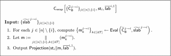

  

  Circuit $\mathsf {C}_\mathsf {wrap}$

• Evaluation: Every party $P_i$ does the following:

  • 1. For each $j \in [n]$,

    • (a) Obtain $(\mathsf {ssid}= j, \widetilde{\mathsf {rlab}}^{j})$ from $\mathcal {F}_{g}$ where party $P_j$ acts as the receiver.

    • (b) $\widetilde{\mathsf {lab}}^{j,1} \leftarrow \mathsf {Eval}(\widetilde{\mathsf {C}}_\mathsf {wrap}^j,\widetilde{\mathsf {rlab}}^{j})$

  • 2. $\mathbf{for}$ each t from 1 to T $\mathbf{do}$:

    • (a) Parse $\phi _t$ as $(i^*,f,g,h)$.

    • (b) Compute $((\alpha ,\beta ,\gamma ),\{\omega ^j\}_{j\in [n]\setminus \{i^*\}},\widetilde{\mathsf {lab}}^{i^*,t+1}) := \mathsf {Eval}(\widetilde{\mathsf {P}}^{i^*,t},\widetilde{\mathsf {lab}}^{i^*,t})$.

    • (c) Set $\mathsf {st}_{i}[h] := \gamma \oplus v_{i}[h]$.

    • (d) $\mathbf{for}$ each $j \ne i^*$ $\mathbf{do}$:

      • i. Compute $(ct = (\delta _0,\delta _1),\{{\mathsf {lab}}^{j,t+1}_{k}\}_{k \in [N] \setminus \{h\}}) := \mathsf {Eval}(\widetilde{\mathsf {P}}^{j,t},\widetilde{\mathsf {lab}}^{j,t})$.

      • ii. Recover $\mathsf {lab}^{j,t+1}_h := \delta _{\gamma } \oplus \omega ^j$.

      • iii. Set $\widetilde{\mathsf {lab}}^{j,t+1} := \{\mathsf {lab}^{j,t+1}_{k}\}_{k \in [N]}$.

  • 3. Compute the output as $\mathsf {post}(i,\mathsf {st}_i)$.

Correctness. In order to prove correctness, it is sufficient to show that the label $\mathsf {lab}^{j,t+1}_h$ computed in Step 2(d)ii of the evaluation procedure corresponds to the bit $\mathsf {NAND}(\mathsf {st}_{i^*}[f] , \mathsf {st}_{i^*}[g])\oplus v_{i^*}[h]$. Notice that by the structure of $v_{i^*}$ we have for every $j \ne i^*$, $\mathsf {st}_j[f] = \mathsf {st}_{i^*}[f] \oplus v_{i^*}[f]$.

First, $\omega ^j$ is computed in Step 2b. Let $k := (t, \alpha , \beta )$, and we have $\omega ^j = \mathsf {m}^{j\rightarrow i^*}_{k} = \mathsf {m}^{j\rightarrow i^*}_{k, \mathsf {PRG}(s_{i^*})[k]}$.

Fig. 6.

The program $\mathsf {P}_{}$

Second, $ct = (\delta _0,\delta _1)$ is computed in Step 2(d)i. Note that $\alpha = \mathsf {st}_{i^*}[f] \oplus v_{i^*}[f] = \mathsf {st}_j[f]$, $\beta = \mathsf {st}_{i^*}[g] \oplus v_{i^*}[g]=\mathsf {st}_j[g]$. From the functionality of $\mathsf {P}^{j,t}$ we know that $ct = ct_{\mathsf {st}_{j}[f],\mathsf {st}_{j}[g]} = ct^j_{\alpha , \beta } =(\mathsf {m}'_{\alpha , \beta , 0} \oplus \mathsf {lab}^{j,t+1}_{h,0}, \mathsf {m}'_{\alpha , \beta , 1} \oplus \mathsf {lab}^{j,t+1}_{h,1}) = (\mathsf {m}^{j \rightarrow i^*}_{k,e_{i^*}[k] } \oplus \mathsf {lab}^{j,t+1}_{h,0}, \mathsf {m}^{j \rightarrow i^*}_{k,e_{i^*}[k]\oplus 1 } \oplus \mathsf {lab}^{j,t+1}_{h,1})$.

Therefore, $\delta _\gamma \oplus \omega ^j = \mathsf {m}^{j \rightarrow i^*}_{k,e_{i^*}[k]\oplus \gamma } \oplus \mathsf {lab}^{j,t+1}_{h,\gamma }\oplus \mathsf {m}^{j\rightarrow i^*}_{k, \mathsf {PRG}(s_{i^*})[k]}$. Recall that $c_{i^*}[k] = \mathsf {NAND}(\mathsf {st}_{i^*}[f] , \mathsf {st}_{i^*}[g])\oplus v_{i^*}[h]=\gamma$, thus $e_{i^*}[k]\oplus \gamma =e_{i^*}[k]\oplus c_{i^*}[k] = \mathsf {PRG}(s_{i^*})[k]$. Hence $\delta _\gamma \oplus \omega ^j = \mathsf {lab}^{j,t+1}_{h,\gamma }$. This concludes the proof.

It is useful to keep in mind that for every $i,j\in [n]$ and $k \in [\ell ]$, we have that $\mathsf {st}_i[k] \oplus v_i[k] = \mathsf {st}_j[k] \oplus v_j[k]$. Let us denote this shared value by $\mathsf {st}^*$. Also, we denote the transcript of the interaction in the computation phase by $\mathsf {Z}$.

Efficiency. Let the number of OT invocations in $\varPhi$ be $\mathsf {npk}_\varPhi$ and in one execution of $\mathcal {F}_g$ be $\mathsf {npk}_{g}$. Since we make non-black box use of the underlying conforming protocol $\varPhi$ (but make black-box use of $\mathcal {F}_g$), we augment the circuit computing $\varPi$ and $\mathcal {F}_g$ to have OT gates (this is similar in spirit to the works of [GMM17a, GMM17b]) to count the number of public-key operations. An OT gate enables one execution of one of the algorithms provided by the OT protocol. We choose the conforming protocol that performs OT extension between every pair of parties so that $\mathsf {npk}_\varPhi$ is bounded by $\mathcal {O}(n^2\lambda )$. Thus, the total number of public-key operations (including the non-black-box public-key operations) in our two-round construction is $\mathcal {O}( \mathsf {npk}_\varPhi + n \cdot \mathsf {npk}_g)$. It follows from Theorem 2 that this number is bounded by $\mathsf {poly}(n,\lambda )$.

Security. The proof of security is given in the full version [GMS18].

5 Special Zero-Knowledge Protocol

In this section, we define and construct a special zero-knowledge protocol which will later be used in our construction against malicious adversaries. We give the formal definition below.

Fig. 7.

Special zero-knowledge functionality $\mathcal {F}_\mathsf {ZK}$

Definition 2

A special zero-knowledge protocol is a two-round protocol that securely realizes the $\mathcal {F}_{\mathsf {ZK}}$ functionality given in Fig. 7. Further, we require the number of pubic key operations performed in the protocol to be bounded by $\mathsf {poly}(n,\lambda )$ independent of the size of x and w.

We give a proof of the following theorem.

Theorem 3

Assuming the existence of two-round UC secure oblivious transfer, there exists a construction of special zero-knowledge protocol.

Fig. 8.

Special zero-knowledge protocol $\varPi _\mathsf {ZK}$

5.1 Construction

We first describe the tools used in the construction.

• 1. Special Non-interactive Statistically Binding Commitment. We use a special non-interactive, statistically binding commitment scheme $(\mathsf {com},\mathsf {decom})$ where the length of the randomness used to commit to arbitrary length messages is $\lambda$. We note that any standard commitment can be made to satisfy this property by using a pseudorandom generator to expand the random string to required length.

• 2. Blum’s Hamiltonicity Protocol. We use the three-round, constant soundness zero-knowledge $(\mathsf {zk}_1,\mathsf {zk}_2,\mathsf {zk}_3)$ protocol of Blum. We note that in Blum’s protocol $\mathsf {zk}_2 \in \{0,1\}$ and we let $\mathsf {zk}_{3,b}$ be the response when $\mathsf {zk}_2 = b$. We also assume without loss of generality that $\mathsf {zk}_1$ includes the instance.

• 3. Two-Round Secure Computation Protocol. We make use of the two-round secure computation protocol of [GS18] (that can be based on any two-round UC secure oblivious transfer) computing the ideal functionality $\mathcal {F}_f$ described in Fig. 10.

• 4. Length Doubling Pseudorandom Generator: We use a pseudorandom generator $\mathsf {PRG}: \{0,1\}^{\lambda } \rightarrow \{0,1\}^{2\lambda }$.

Fig. 9.

Circuit C

Fig. 10.

The function f computed by the internal MPC

Overview. We present the formal construction in the $\mathcal {F}_f$ hybrid model in Fig. 8.

Correctness. To argue the correctness of the protocol, we only need to prove that in the evaluation step, $\mu$ is either $\mu _0$ or $\mu _1$ based on whether $R(x,w) = 0$ or $R(x,w)=1$. We know that the output of $\mathcal {F}_f$ is $\left\{ \mathsf {lab}^{i}_w\right\} _{i,w \in [\lambda ]}$, where $\mathsf {lab}^i_w = \mathsf {lab}^i_{w,r^i_{ch[i]}[w]}$. Notice that $\mathsf {lab}^i_{w,b}$’s are the input keys of $\widetilde{C}$, hence $\mathsf {lab}^i_w$ is the label corresponding to the w-th bit of $r^i_{ch[i]}$. Using these input labels to evaluate $\widetilde{C}$ gives us $\mathsf {Eval}\left( \widetilde{C}, \left\{ \mathsf {lab}^{i}_w\right\} _{i,w \in [\lambda ]}\right) = C\left( \left\{ r^i_{ch[i]} \right\} _{i \in [\lambda ]}\right)$.

In the circuit evaluation of C, $r^i_{ch[i]}$ is used to obtain $\mathsf {zk}^i_{3,ch[i]}$ from $c^i_{ch[i]}$. It now follows from the completeness of $(\mathsf {zk}^i_1,ch[i],\mathsf {zk}^{i}_{3,ch[i]})$ that $\mu$ is either $\mu _0$ or $\mu _1$ based on $R(x,w) = 0$ or $R(x,w) = 1$.

Efficiency. The number of public key operations performed in the protocol is $\mathsf {poly}(n,\lambda )$ which follows from Theorem 2 when applied to function f.

Security. We give the security proof in the full version [GMS18].

6 Malicious Secure Protocol

In this section, we give a construction of two-round, multiparty computation that is secure against malicious adversaries and minimizes the number of public key operations.

6.1 Construction

Our two-round protocol computing a function f uses the following primitives.

• 1. An n-party malicious secure conforming protocol $\varPhi$ computing the function f.

• 2. A selective garbling scheme for circuits $(\mathsf {Garble},\mathsf {Eval})$.

• 3. A pseudorandom generator $\mathsf {PRG}_{\mathsf {mal}}: \{0,1\}^{\lambda } \rightarrow \{0,1\}^{4T}$ where each output bit can be computed by a circuit of size $\mathsf {poly}(\lambda ,\log {T})$.⁵

• 4. A somewhere adaptive garbling scheme for circuits $(\mathsf {SAdpGarbleCkt},\mathsf {SAdpGarbleInp},\mathsf {SAdpEvalCkt})$ (defined in Sect. 3.2). We assume that the length of the garbled input when $\mathsf {SAdpGarbleCkt}$ is used to garbled $\mathsf {C}_{\mathsf {B}}$ (described in Fig. 11) is M.

• 5. A maliciously secure two-round MPC protocol computing the function g described in Fig. 12.

• 6. A non-interactive statistically binding commitment scheme $(\mathsf {Com},\mathsf {Decom})$.

• 7. The special ZK protocol parameterized by an $\mathsf {NP}$ relation R described below.

  $$\begin{aligned} R:= & {} \Bigg \{\left( x = \left( \widetilde{\mathsf {C}}_{\mathsf {B}}, \mathsf {cm}\right) , w = \left( \varOmega , \mathsf {C}_{\mathsf {B}},\mathsf {state}, \omega \right) \right) : \\&\quad \left( \mathsf {Decom}(\mathsf {cm},\mathsf {state},\omega ) = 1 \right) \wedge \left( (\widetilde{\mathsf {C}}_{\mathsf {B}},\mathsf {state}) = \mathsf {SAdpGarbleCkt}\left( \mathsf {C}_{\mathsf {B}}; \varOmega \right) \right) \Bigg \}. \end{aligned}$$

Description of the Protocol. We now give a formal description of our construction in below in the $\mathcal {F}_{g}$ and $\mathcal {F}_{\mathsf {zk}}$ hybrid model.

• Round-1: Each party $P_i$ does the following:

  • 1. Compute $(z_i,v_i) \leftarrow \mathsf {pre}(1^{\lambda },i,x_i)$.

  • 2. For each $t \in [T]$ and for each $\alpha ,\beta \in \{0,1\}$

    $$c_i[(t,\alpha ,\beta )] := v_i[h] \oplus \mathsf {NAND}(v_i[f]\oplus \alpha ,v_i[g] \oplus \beta )$$

    where $\phi _t = (\star ,f,g,h)$.

  • 3. Sample $s_i \leftarrow \{0,1\}^\lambda$ and compute $e_i := \mathsf {PRG}_{\mathsf {mal}}(s_i) \oplus c_i$.

  • 4. For each $j \in [n] \setminus \{i\}$, sample

    $$\begin{aligned} \mu ^{j\rightarrow i}_0,\mu ^{j\rightarrow i}_1\leftarrow & {} \{0,1\}^{\lambda } \\ \mathsf {rlab}_{k,b}^{j \rightarrow i}\leftarrow & {} \{0,1\}^\lambda \text { for all } k \in [M], b\in \{0,1\}\\ \mathsf {m}^{i \rightarrow j}_{k,b}\leftarrow & {} \{0,1\}^{\lambda } \text { for all } k\in [4T], b \in \{0,1\}\end{aligned}$$

  • 5. Garbling $\mathsf {C}_{\mathsf {B}}$: For each $j \in [n] \setminus \{i\}$, compute

    $$\begin{aligned} (\widetilde{\mathsf {C}}^{i \rightarrow j}_\mathsf {B},\mathsf {state}^{i\rightarrow j}):= & {} \mathsf {SAdpGarbleCkt}\left( \mathsf {C}_{\mathsf {B}} \left[ \left\{ \mathsf {m}^{i \rightarrow j}_{k,0},\mathsf {m}^{i \rightarrow j}_{k,1}\right\} _{k\in [4T], b\in \{0,1\}}\right] ; \varOmega \right) \\ \mathsf {cm}^{i \rightarrow j}:= & {} \mathsf {Com}(\mathsf {state}^{i \rightarrow j}; \omega ^{i \rightarrow j}) \end{aligned}$$

    where $\mathsf {C}_{\mathsf {B}}$ is described in Fig. 11 and $\varOmega ,\omega ^{i \rightarrow j}$ are sampled randomly.

  • 6. Messages to $\mathcal {F}_g$: Send $(\mathsf {ssid}= i, s_i, \{\mathsf {rlab}^{j \rightarrow i}_{k,b}\}_{j \in [n]\setminus \{i\},k\in [M],b \in \{0,1\}})$ to $\mathcal {F}_g$ acting as the receiver and for each $j \in [n] \setminus \{i\}$, send $(\mathsf {ssid}= j,\{\mathsf {cm}^{i \rightarrow j}, \mathsf {state}^{i \rightarrow j}, \omega ^{i \rightarrow j}\})$ to $\mathcal {F}_g$ acting as the sender.

  • 7. Messages to $\mathcal {F}_{\mathsf {zk}}$: For each $j \in [n] \setminus \{i\}$, send $(\mathsf {ssid}= (j\rightarrow i), \mu ^{j\rightarrow i}_0,\mu ^{j\rightarrow i}_1)$ to $\mathcal {F}_{\mathsf {zk}}$ acting as the verifier, and send $(\mathsf {ssid}= (i\rightarrow j), X^{i \rightarrow j},W^{i \rightarrow j})$ to $\mathcal {F}_{\mathsf {zk}}$ acting as the prover where $X^{i \rightarrow j} = \left( \widetilde{\mathsf {C}}^{i \rightarrow j}_{\mathsf {B}}, \mathsf {cm}^{i \rightarrow j} \right)$ and $W^{i \rightarrow j} = \Big ( \varOmega , \mathsf {C}_{\mathsf {B}}\left[ \left\{ \mathsf {m}^{i \rightarrow j}_{k,0},\mathsf {m}^{i \rightarrow j}_{k,1}\right\} _{k\in [4T], b\in \{0,1\}}\right] ,\mathsf {state}^{i \rightarrow j},\omega ^{i \rightarrow j}\Big )$.

  • 8. Send $\left( z_i, \{\widetilde{\mathsf {C}}^{i \rightarrow j}_\mathsf {B}\}_{j \in [n]\setminus \{i\}},e_i, \{\mathsf {cm}^{i \rightarrow j}\}_{j \in [n]\setminus \{i\}}\right)$ to every other party.

  Fig. 11.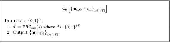

  

  Circuit $\mathsf {C}_{\mathsf {B}}$

• Round-2: Each party $P_i$ does the following:

  • 1. Set $\mathsf {st}_i := \left( z_1 \Vert \ldots \Vert z_n \right) \oplus v_i$.

  • 2. Set $N = \ell + 4T\lambda (n-1)$.

  • 3. Set $\overline{\mathsf {lab}}^{i,T+1} := \{\mathsf {lab}_{k,0}^{i,T+1}, \mathsf {lab}_{k,1}^{i,T+1}\}_{k\in [N]}$ where $\mathsf {lab}_{k,b}^{i,T+1} := 0^\lambda$ for each $k \in [N],b \in \{0,1\}$.

  • 4. $\mathbf{for}$ each t from T down to 1 $\mathbf{do}$:

    • (a) Parse $\phi _t$ as $(i^*,f,g,h)$.

    • (b) If $i = i^*$ then compute (where $\mathsf {P}$ is described in Fig. 6)

      $$\big (\widetilde{\mathsf {P}}^{i,t}, \overline{\mathsf {lab}}^{i,t} \big ) \leftarrow \mathsf {Garble}(1^{\lambda },\mathsf {P}[{i,\phi _t},v_i,\bot ,\overline{\mathsf {lab}}^{i,t+1}]).$$

    • (c) If $i \ne i^*$ then for every $\alpha ,\beta \in \{0,1\}$, set $\mathsf {m}'_{\alpha ,\beta ,0} = \mathsf {m}^{i \rightarrow i^*}_{(t,\alpha ,\beta ),e_{i^*}[(t,\alpha ,\beta )]}$ and $\mathsf {m}'_{\alpha ,\beta ,1} = \mathsf {m}^{i \rightarrow i^*}_{(t,\alpha ,\beta ),1 \oplus e_{i^*}[(t,\alpha ,\beta )]}$. Compute $ct^{i }_{t,\alpha ,\beta } := (\mathsf {m}'_{\alpha ,\beta ,0} \oplus \mathsf {lab}^{i,t+1}_{h,0}, \mathsf {m}'_{\alpha ,\beta ,1} \oplus \mathsf {lab}^{i,t+1}_{h,1})$ and compute

      $$\big (\widetilde{\mathsf {P}}^{i,t}, \overline{\mathsf {lab}}^{i,t} \big ) \leftarrow \mathsf {Garble}(1^{\lambda },\mathsf {P}[{i,\phi _t},v_i,\{ct^{i }_{t,\alpha ,\beta }\},\overline{\mathsf {lab}}^{i,t+1}]).$$

  • 5. Garbling $\mathsf {C}_{\mathsf {wrap}}$: Compute

    $$\begin{aligned} \widetilde{\mathsf {C}}^i_{\mathsf {wrap}}\leftarrow \mathsf {Garble}&\Big (\mathsf {C}_{\mathsf {wrap}}\left[ \{\widetilde{\mathsf {C}}^{j \rightarrow i}_{\mathsf {B}}\}_{j \in [n] \setminus \{i\}}, \mathsf {st}_i,\overline{\mathsf {lab}}^{i,1}\right] ,\\&\left\{ \{\mu ^{j\rightarrow i}_b\}_{j\in [n]\setminus \{i\}},\{\mathsf {rlab}^{j \rightarrow i}_{k,b}\}_{j \in [n] \setminus \{i\},k \in [M],b \in \{0,1\}} \right\} \Big ) \end{aligned}$$

    where $\mathsf {C}_{\mathsf {wrap}}$ is described in Fig. 13.

  • 6. Send $\left( \{\widetilde{\mathsf {P}}^{i,t}\}_{t \in [T]}, \widetilde{\mathsf {C}}^i_{\mathsf {wrap}}\right)$ to every other party.

  Fig. 12.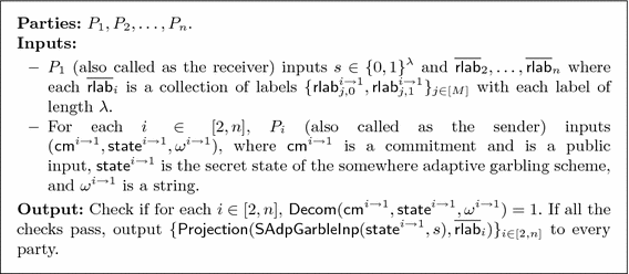

  

  The function g computed by the internal MPC where $P_1$ acts as the receiver

  Fig. 13.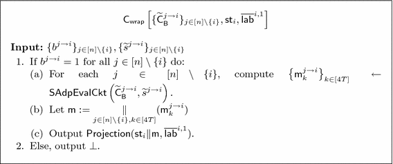

  

  Circuit $\mathsf {C}^{\mathsf {wrap}}$

• Evaluation: Every party $P_i$ does the following:

  • 1. For each $j \in [n]$,

    • (a) Obtain $(\mathsf {ssid}= j, \{\widetilde{\mathsf {rlab}}^{j}\})$ from $\mathcal {F}_{g}$ where party $P_j$ acts as the receiver.

    • (b) For each $k \in [n] \setminus \{j\}$, obtain $(\mathsf {ssid}=(k\rightarrow j), b^{k \rightarrow j}, X^{k \rightarrow j}, \mu ^{k\rightarrow j})$ from $\mathcal {F}_{\mathsf {zk}}$. Set $\widetilde{\mu }^j = \{\mu ^{k\rightarrow j}\}_{k \in [n] \setminus \{j\}}$.

    • (c) $\widetilde{\mathsf {lab}}^{j,1} \leftarrow \mathsf {Eval}(\widetilde{\mathsf {C}}^j_{\mathsf {wrap}},\widetilde{\mu }^j \Vert \widetilde{\mathsf {rlab}}^{j})$.

  • 2. $\mathbf{for}$ each t from 1 to T $\mathbf{do}$:

    • (a) Parse $\phi _t$ as $(i^*,f,g,h)$.

    • (b) Compute $((\alpha ,\beta ,\gamma ),\{\omega ^j\}_{j\in [n]\setminus \{i\}},\widetilde{\mathsf {lab}}^{i^*,t+1}) := \mathsf {Eval}(\widetilde{\mathsf {P}}^{i^*,t},\widetilde{\mathsf {lab}}^{i^*,t})$.

    • (c) Set $\mathsf {st}_{i}[h] := \gamma \oplus v_{i}[h]$.

    • (d) $\mathbf{for}$ each $j \ne i^*$ $\mathbf{do}$:

      • i. Compute $(ct = (\delta _0,\delta _1),\{{\mathsf {lab}}^{j,t+1}_{k}\}_{k \in [N] \setminus \{h\}}) := \mathsf {Eval}(\widetilde{\mathsf {P}}^{j,t},\widetilde{\mathsf {lab}}^{j,t})$.

      • ii. Recover $\mathsf {lab}^{j,t+1}_h := \delta _{\gamma } \oplus \omega ^j$.

      • iii. Set $\widetilde{\mathsf {lab}}^{j,t+1} := \{\mathsf {lab}^{j,t+1}_{k}\}_{k \in [N]}$.

  • 3. Compute the output as $\mathsf {post}(i,\mathsf {st}_i)$.

Correctness. The correctness follows via a similar argument to the semi-honest case.

Efficiency. Let the number of public key operations in $\varPhi$ be $\mathsf {npk}_\varPhi$, in one execution of $\mathcal {F}_{\mathsf {zk}}$ be $\mathsf {npk}_{\mathsf {zk}}$, and in one execution of $\mathcal {F}_g$ be $\mathsf {npk}_{g}$. We choose the conforming protocol that performs OT extension between every pair of parties so that $\mathsf {npk}_\varPhi$ is bounded by $\mathcal {O}(n^2\lambda )$. The total number of public key operations in our two-round construction is $\mathcal {O}(\mathsf {npk}_\varPhi + n^2 \cdot \mathsf {npk}_{\mathsf {zk}} + n \cdot \mathsf {npk}_g)$. It follows from Theorems 3, 2 that this number is bounded by $\mathsf {poly}(n,\lambda )$.

Security. The security proof will be given in the full version [GMS18].

References

Ananth, P., Choudhuri, A.R., Jain, A.: A new approach to round-optimal secure multiparty computation. In: Katz, J., Shacham, H. (eds.) CRYPTO 2017, Part I. LNCS, vol. 10401, pp. 468–499. Springer, Cham (2017). https://doi.org/10.1007/978-3-319-63688-7_16
Applebaum, B., Ishai, Y., Kushilevitz, E., Waters, B.: Encoding functions with constant online rate or how to compress garbled circuits keys. In: Canetti, R., Garay, J.A. (eds.) CRYPTO 2013, Part II. LNCS, vol. 8043, pp. 166–184. Springer, Heidelberg (2013). https://doi.org/10.1007/978-3-642-40084-1_10
Asharov, G., Lindell, Y., Schneider, T., Zohner, M.: More efficient oblivious transfer extensions. J. Cryptol. 30(3), 805–858 (2017)
Beaver, D.: Correlated pseudorandomness and the complexity of private computations. In: Proceedings of the Twenty-Eighth Annual ACM Symposium on the Theory of Computing, Philadelphia, Pennsylvania, 22–24 May 1996, pp. 479–488 (1996)
Boyle, E., Gilboa, N., Ishai, Y.: Breaking the circuit size barrier for secure computation under DDH. In: Robshaw, M., Katz, J. (eds.) CRYPTO 2016, Part I. LNCS, vol. 9814, pp. 509–539. Springer, Heidelberg (2016). https://doi.org/10.1007/978-3-662-53018-4_19
Badrinarayanan, S., Garg, S., Ishai, Y., Sahai, A., Wadia, A.: Two-message witness indistinguishability and secure computation in the plain model from new assumptions. In: Takagi, T., Peyrin, T. (eds.) ASIACRYPT 2017, Part III. LNCS, vol. 10626, pp. 275–303. Springer, Cham (2017). https://doi.org/10.1007/978-3-319-70700-6_10
Boyle, E., Gilboa, N., Ishai, Y.: Group-based secure computation: optimizing rounds, communication, and computation. In: Coron, J.-S., Nielsen, J.B. (eds.) EUROCRYPT 2017, Part II. LNCS, vol. 10211, pp. 163–193. Springer, Cham (2017). https://doi.org/10.1007/978-3-319-56614-6_6
Badrinarayanan, S., Goyal, V., Jain, A., Kalai, Y.T., Khurana, D., Sahai, A.: Promise zero knowledge and its applications to round optimal MPC. Cryptology ePrint Archive, Report 2017/1088 (2017). https://eprint.iacr.org/2017/1088
Brakerski, Z., Halevi, S., Polychroniadou, A.: Four round secure computation without setup. In: Kalai, Y., Reyzin, L. (eds.) TCC 2017, Part I. LNCS, vol. 10677, pp. 645–677. Springer, Cham (2017). https://doi.org/10.1007/978-3-319-70500-2_22
Bellare, M., Hoang, V.T., Rogaway, P.: Foundations of garbled circuits. In: Yu, T., Danezis, G., Gligor, V.D., (eds.) ACM CCS 2012, pp. 784–796. ACM Press, October 2012
Benhamouda, F., Lin, H.: k-round MPC from k-round OT via garbled interactive circuits. In: EUROCRYPT (2018, to appear). https://eprint.iacr.org/2017/1125
Beaver, D., Micali, S., Rogaway, P.: The round complexity of secure protocols (extended abstract). In: 22nd ACM STOC, pp. 503–513. ACM Press, May 1990
Brakerski, Z., Perlman, R.: Lattice-based fully dynamic multi-key FHE with short ciphertexts. In: Robshaw, M., Katz, J. (eds.) CRYPTO 2016, Part I. LNCS, vol. 9814, pp. 190–213. Springer, Heidelberg (2016). https://doi.org/10.1007/978-3-662-53018-4_8
Canetti, R.: Security and composition of multiparty cryptographic protocols. J. Cryptol. 13(1), 143–202 (2000)
Canetti, R.: Universally composable security: a new paradigm for cryptographic protocols. Cryptology ePrint Archive, Report 2000/067 (2000). http://eprint.iacr.org/2000/067
Canetti, R.: Universally composable security: a new paradigm for cryptographic protocols. In: 42nd FOCS, pp. 136–145. IEEE Computer Society Press, October 2001
Ciampi, M., Ostrovsky, R., Siniscalchi, L., Visconti, I.: Round-optimal secure two-party computation from trapdoor permutations. In: Kalai, Y., Reyzin, L. (eds.) TCC 2017, Part I. LNCS, vol. 10677, pp. 678–710. Springer, Cham (2017). https://doi.org/10.1007/978-3-319-70500-2_23
Feige, U., Shamir, A.: Witness indistinguishable and witness hiding protocols. In: 22nd ACM STOC, pp. 416–426. ACM Press, May 1990
Garg, S., Gentry, C., Halevi, S., Raykova, M., Sahai, A., Waters, B.: Candidate indistinguishability obfuscation and functional encryption for all circuits. In: 54th FOCS, pp. 40–49. IEEE Computer Society Press, October 2013
Garg, S., Gentry, C., Halevi, S., Raykova, M.: Two-round secure MPC from indistinguishability obfuscation. In: Lindell, Y. (ed.) TCC 2014. LNCS, vol. 8349, pp. 74–94. Springer, Heidelberg (2014). https://doi.org/10.1007/978-3-642-54242-8_4
Goldreich, O., Goldwasser, S., Micali, S.: How to construct random functions. J. ACM 33(4), 792–807 (1986)
Garg, S., Gentry, C., Sahai, A., Waters, B.: Witness encryption and its applications. In: Boneh, D., Roughgarden, T., Feigenbaum, J. (eds.) 45th ACM STOC, pp. 467–476. ACM Press, June 2013
Dov Gordon, S., Liu, F.-H., Shi, E.: Constant-round MPC with fairness and guarantee of output delivery. In: Gennaro, R., Robshaw, M. (eds.) CRYPTO 2015, Part II. LNCS, vol. 9216, pp. 63–82. Springer, Heidelberg (2015). https://doi.org/10.1007/978-3-662-48000-7_4
Garg, S., Mahmoody, M., Mohammed, A.: Lower bounds on obfuscation from all-or-nothing encryption primitives. In: Katz, J., Shacham, H. (eds.) CRYPTO 2017, Part I. LNCS, vol. 10401, pp. 661–695. Springer, Cham (2017). https://doi.org/10.1007/978-3-319-63688-7_22
Garg, S., Mahmoody, M., Mohammed, A.: When does functional encryption imply obfuscation? In: Kalai, Y., Reyzin, L. (eds.) TCC 2017, Part I. LNCS, vol. 10677, pp. 82–115. Springer, Cham (2017). https://doi.org/10.1007/978-3-319-70500-2_4
Garg, S., Mahmoody, M., Masny, D., Meckler, I.: On the round complexity of OT extension. Cryptology ePrint Archive, Report 2017/1187 (2017). https://eprint.iacr.org/2017/1187
Garg, S., Mukherjee, P., Pandey, O., Polychroniadou, A.: The exact round complexity of secure computation. In: Fischlin, M., Coron, J.-S. (eds.) EUROCRYPT 2016, Part II. LNCS, vol. 9666, pp. 448–476. Springer, Heidelberg (2016). https://doi.org/10.1007/978-3-662-49896-5_16
Garg, S., Miao, P., Srinivasan, A.: Two-round multiparty secure computation minimizing public key operations. Cryptology ePrint Archive, Report 2018/180 (2018). https://eprint.iacr.org/2018/180
Goldreich, O., Micali, S., Wigderson, A.: How to play any mental game or a completeness theorem for protocols with honest majority. In: Aho, A. (ed.) 19th ACM STOC, pp. 218–229. ACM Press, May 1987
Garg, S., Srinivasan, A.: Garbled protocols and two-round MPC from bilinear maps. In: 58th FOCS, pp. 588–599. IEEE Computer Society Press (2017)
Garg, S., Srinivasan, A.: Two-round multiparty secure computation from minimal assumptions. In: Nielsen, J.B., Rijmen, V. (eds.) EUROCRYPT 2018. LNCS, vol. 10821, pp. 468–499. Springer, Cham (2018). https://doi.org/10.1007/978-3-319-78375-8_16. https://eprint.iacr.org/2017/1156
Halevi, S., Hazay, C., Polychroniadou, A., Venkitasubramaniam, M.: Round-optimal secure multi-party computation. Cryptology ePrint Archive, Report 2017/1056 (2017). http://eprint.iacr.org/2017/1056
Harnik, D., Ishai, Y., Kushilevitz, E.: How many oblivious transfers are needed for secure multiparty computation? In: Menezes, A. (ed.) CRYPTO 2007. LNCS, vol. 4622, pp. 284–302. Springer, Heidelberg (2007). https://doi.org/10.1007/978-3-540-74143-5_16
Harnik, D., Ishai, Y., Kushilevitz, E., Nielsen, J.B.: OT-combiners via secure computation. In: Canetti, R. (ed.) TCC 2008. LNCS, vol. 4948, pp. 393–411. Springer, Heidelberg (2008). https://doi.org/10.1007/978-3-540-78524-8_22
Hemenway, B., Jafargholi, Z., Ostrovsky, R., Scafuro, A., Wichs, D.: Adaptively secure garbled circuits from one-way functions. In: Robshaw, M., Katz, J. (eds.) CRYPTO 2016, Part III. LNCS, vol. 9816, pp. 149–178. Springer, Heidelberg (2016). https://doi.org/10.1007/978-3-662-53015-3_6
Halevi, S., Lindell, Y., Pinkas, B.: Secure computation on the web: computing without simultaneous interaction. In: Rogaway, P. (ed.) CRYPTO 2011. LNCS, vol. 6841, pp. 132–150. Springer, Heidelberg (2011). https://doi.org/10.1007/978-3-642-22792-9_8
Ishai, Y., Kilian, J., Nissim, K., Petrank, E.: Extending oblivious transfers efficiently. In: Boneh, D. (ed.) CRYPTO 2003. LNCS, vol. 2729, pp. 145–161. Springer, Heidelberg (2003). https://doi.org/10.1007/978-3-540-45146-4_9
Jafargholi, Z., Kamath, C., Klein, K., Komargodski, I., Pietrzak, K., Wichs, D.: Be adaptive, avoid overcommitting. In: Katz, J., Shacham, H. (eds.) CRYPTO 2017, Part I. LNCS, vol. 10401, pp. 133–163. Springer, Cham (2017). https://doi.org/10.1007/978-3-319-63688-7_5
Jain, A., Kalai, Y.T., Khurana, D., Rothblum, R.: Distinguisher-dependent simulation in two rounds and its applications. In: Katz, J., Shacham, H. (eds.) CRYPTO 2017, Part II. LNCS, vol. 10402, pp. 158–189. Springer, Cham (2017). https://doi.org/10.1007/978-3-319-63715-0_6
Jafargholi, Z., Wichs, D.: Adaptive security of Yao’s garbled circuits. In: Hirt, M., Smith, A. (eds.) TCC 2016, Part I. LNCS, vol. 9985, pp. 433–458. Springer, Heidelberg (2016). https://doi.org/10.1007/978-3-662-53641-4_17
Kolesnikov, V., Kumaresan, R.: Improved OT extension for transferring short secrets. In: Canetti, R., Garay, J.A. (eds.) CRYPTO 2013, Part II. LNCS, vol. 8043, pp. 54–70. Springer, Heidelberg (2013). https://doi.org/10.1007/978-3-642-40084-1_4
Kumaresan, R., Raghuraman, S., Sealfon, A.: Network oblivious transfer. In: Robshaw, M., Katz, J. (eds.) CRYPTO 2016, Part II. LNCS, vol. 9815, pp. 366–396. Springer, Heidelberg (2016). https://doi.org/10.1007/978-3-662-53008-5_13
Lindell, Y., Pinkas, B.: A proof of security of Yao’s protocol for two-party computation. J. Cryptol. 22(2), 161–188 (2009)
Mukherjee, P., Wichs, D.: Two round multiparty computation via multi-key FHE. In: Fischlin, M., Coron, J.-S. (eds.) EUROCRYPT 2016, Part II. LNCS, vol. 9666, pp. 735–763. Springer, Heidelberg (2016). https://doi.org/10.1007/978-3-662-49896-5_26
Nielsen, J.B.: Extending oblivious transfers efficiently - how to get robustness almost for free. Cryptology ePrint Archive, Report 2007/215 (2007). http://eprint.iacr.org/2007/215
Nielsen, J.B., Nordholt, P.S., Orlandi, C., Burra, S.S.: A new approach to practical active-secure two-party computation. In: Safavi-Naini, R., Canetti, R. (eds.) CRYPTO 2012. LNCS, vol. 7417, pp. 681–700. Springer, Heidelberg (2012). https://doi.org/10.1007/978-3-642-32009-5_40
Peikert, C., Shiehian, S.: Multi-key FHE from LWE, revisited. In: Hirt, M., Smith, A. (eds.) TCC 2016, Part II. LNCS, vol. 9986, pp. 217–238. Springer, Heidelberg (2016). https://doi.org/10.1007/978-3-662-53644-5_9
Yao, A.C.-C.: Protocols for secure computations (extended abstract). In: 23rd FOCS, pp. 160–164. IEEE Computer Society Press, November 1982
Author information
Authors and Affiliations
Corresponding author
Editor information
Editors and Affiliations
Rights and permissions
Copyright information
© 2018 International Association for Cryptologic Research
About this paper
Cite this paper
Garg, S., Miao, P., Srinivasan, A. (2018). Two-Round Multiparty Secure Computation Minimizing Public Key Operations. In: Shacham, H., Boldyreva, A. (eds) Advances in Cryptology – CRYPTO 2018. CRYPTO 2018. Lecture Notes in Computer Science(), vol 10993. Springer, Cham. https://doi.org/10.1007/978-3-319-96878-0_10
Download citation
DOI: https://doi.org/10.1007/978-3-319-96878-0_10
Published:
Publisher Name: Springer, Cham
Print ISBN: 978-3-319-96877-3
Online ISBN: 978-3-319-96878-0
eBook Packages: Computer ScienceComputer Science (R0)