Metric Temporal Graph Logic over Typed Attributed Graphs

Abstract

Various kinds of typed attributed graphs can be used to represent states of systems from a broad range of domains. For dynamic systems, established formalisms such as graph transformation can provide a formal model for defining state sequences. We consider the case where time may elapse between state changes and introduce a logic, called Metric Temporal Graph Logic (MTGL), to reason about such timed graph sequences. With this logic, we express properties on the structure and attributes of states as well as on the occurrence of states over time that are related by their inner structure, which no formal logic over graphs concisely accomplishes so far.

Firstly, based on timed graph sequences as models for system evolution, we define MTGL by integrating the temporal operator until with time bounds into the well-established logic of (nested) graph conditions. Secondly, we outline how a finite timed graph sequence can be represented as a single graph containing all changes over time (called graph with history), how the satisfaction of MTGL conditions can be defined for such a graph and show that both representations satisfy the same MTGL conditions. Thirdly, we present how MTGL conditions can be reduced to (nested) graph conditions and show using this reduction that both underlying logics are equally expressive. Finally, we present an extension of the tool $\textsc {AutoGraph}$ allowing to check the satisfaction of MTGL conditions for timed graph sequences, by checking the satisfaction of the (nested) graph conditions, obtained using the proposed reduction, for the graph with history corresponding to the timed graph sequence.

1 Introduction

Various kinds of typed attributed graphs are used to represent states of systems from a broad range of domains. Also, the evolution of such systems can be described using a multitude of graph transformation formalisms in which the possible behavior in form of graph sequences is defined by a set of rules and their application. In many cases, the analysis of this induced behavior with respect to a specification in form of a temporal logic that defines the admissible graph sequences is of paramount importance.

In our running example, from which we derive the lack of suitable specification formalisms, we consider a dynamic system describing an operating system, which generates timed sequences of (typed attributed) graphs to model the change of the operating system states over time. In this example, users may create tasks with identifiers $id$, the operating system may create handlers specific to task identifiers to allow for the task execution, and the handlers may produce a result when a task has been executed (marking the successful handling of the task). To model the states of the operating system, we employ graphs that store the tasks, the handlers, and the computed results. In the remainder, we refer in the context of this example to the sequence property P to be checked w.r.t. the timed graph sequence at hand describing systems’ state changes over time.

P::

Whenever a task T with identifier $id$ is created on a system S, a handler H for this task (i.e., with a task identifier $t\_id$ equal to $id$ of T) must exist. Moreover, within 120 timeunits, the handler must produce a result R with value $success$ and, during the computation of the result, no other handler $H'$ for the same task (i.e., with the same task identifier $t\_id$) may exist.

We consider the problem that existing specification formalisms for graph-based systems cannot cover properties such as P. The available (metric) temporal logics, such as Metric Temporal Logic (MTL) [16], are defined over Kripke structures abstracting from the system states by labeling each state with a subset of the finite set of atomic propositions. The commonly used operator until allows then to formalize the part of property P stating that every graph that contains a task T is followed by some graph containing some result R before t time units. However, the existing metric temporal logics do not support the use of bindings of elements contained in the graphs to express how a certain matched pattern evolves in a sequence of graphs. Therefore, they are insufficient when e.g. creating different tasks T and $T'$ must be followed by creating the corresponding results R and $R'$ while also treating the deadlines for their existence separately.

As a first contribution, we define Metric Temporal Graph Logic (MTGL) for the concise specification of systems that generate timed graph sequences. In MTGL, we express properties on states using the well-known formalism of nested graph conditions [12, 24] (called GCs for short). The satisfaction of a GC that states the existence of a graph pattern H in the given graph G results in a match m from H to G. We extend the logic of GCs to MTGL by extending GCs with the metric temporal operator until that may appear in the scope of a previously determined match m. Using this extension, we can express properties, such as property P, on the structure and attributes of states as well as on the occurrence of states over time where the preservation/extension of matches during a systems’ evolution increases the expressiveness beyond the existing formal logics.

As a second contribution, we outline how a finite timed graph sequence can be represented as a single graph containing all changes over time (called graph with history), how the satisfaction of MTGL conditions can be defined for such a graph, and show that both representations satisfy the same MTGL conditions.

As a third contribution, we show that MTGL conditions can be reduced to GCs using attribute constraints to encode the metric temporal requirements, while preserving the satisfaction for finite timed graph sequences. This encoding enables the direct application of techniques for GCs such as [25].

As a fourth contribution, we present an extension of the tool $\textsc {AutoGraph}$  [25] allowing to check the satisfaction of MTGL conditions for timed graph sequences by checking the satisfaction of the GCs obtained using the proposed reduction for the graph with history corresponding to the timed graph sequence at hand.

The paper is structured as follows. Section 2 discusses related work. Section 3 iterates on technical preliminaries. Section 4 defines timed graph sequences, MTGL, and the satisfaction of MTGL conditions for timed graph sequences. In Sect. 5, we show how to represent a finite timed graph sequence as a single graph with history, define satisfaction of MTGL conditions for a graph with history, and prove that both representations satisfy the same MTGL conditions. In Sect. 6, we introduce a reduction of MTGL conditions to GCs and show the equivalence of these two logics. Finally, Sect. 7 discusses the tool support and Sect. 8 concludes the paper with a summary and remarks on future work.

2 Related Work

There are several related formal and informal approaches for the specification and verification of different kinds of sequence properties.

In [13] the satisfaction of CTL (state/sequence) properties is checked where the tool Groove [10, 26] is used to generate the finite state space of the graph transformation system (GTS) at hand. In [7] invariants are checked for a GTS with a possibly infinite state space. The validity of given pre/post conditions for a program over a GTS has been presented in [23]. In [2, 15] temporal properties for GTS with infinite state space are checked using the tool Augur2.

In [19] the satisfaction of graph-based probabilistic timed CTL properties is checked where the tool Henshin [1, 8] is used to generate the finite state space of a GTS and where the tool Prism [17] is used to model check translations of the given properties. In [6] a sequence of timed events are checked against sequence properties given by regular languages based on deterministic finite automata.

The use of bindings, as in this paper, is supported in [3] where bindings are part of the Metric First-Order Temporal Logic in which system states are represented by a set of relations that are adapted during the execution of the system.

A visual but informal notation for the specification of sequence properties involving time and graph bindings was introduced in [14].

In conclusion, existing approaches with a formal semantics do not support either time, bindings, or graphs in a concise manner. Thereby, our graph-based logic MTGL  for graph-based systems complements existing approaches since (a) it eases usability in graph-based contexts similarly to the usage of GCs that are favored over first-order logic in these contexts, (b) it enables further developments and combinations with other graph-based techniques such as those in [25], and, (c) as to be shown by future tool-based evaluations, it can be expected that domain-specific tools for checking MTGL conditions are more efficient compared to general-purpose tools such as shown analogously for GCs in [23].

Fig. 1.

The type graph $TG$ for our running example where the attributes ${\text {cts}}$ and ${\text {dts}}$ of sort $\mathsf {real}$ used in later sections are omitted in every node and edge to improve readability

3 Typed Attributed Graphs and Graph Conditions

We now recall typed attributed graphs and nested graph conditions used for representing system states and properties on these states, respectively.

We use symbolic graphs [21] to encode (finite) typed attributed graphs. Symbolic graphs are an adaptation of E-Graphs  [9] where a graph does not contain data nodes (i.e., elements that represent actual values) but instead node and edge attributes are connected to variables, which replace the data nodes. Symbolic graphs are also equipped with attribute constraints over these (sorted) variables (e.g. $x=5$, $x\le 5$, and y = “aabb”).

We consider symbolic graphs that are typed over a type graph $TG$ using a typing morphism $type :G\rightarrow TG$. Type graphs restrict attributed graphs to an admitted subset. For our running example, we employ the type graph $TG$ from Fig. 1. An example of a symbolic graph that is typed over $TG$ is given in Fig. 4.

We state the existence and nonexistence of graph patterns in a given symbolic graph, which is called a host graph, by representing graph patterns by symbolic graphs and by using monomorphisms (called monos and denoted using subsequently) to extend graph patterns. Formally, we rely on the notion of nested graph conditions (GCs) [12], which are expressively equivalent to first-order logic on graphs [5] as shown in [12, 24].

Definition 1

(Graph Conditions (GCs)). The class of graph conditions (GCs) $\varPhi ^{\mathrm {GC}} _H$ for the graph H contains $\psi$ if one of the following cases applies.

• $\psi =\wedge S$ and $S=\{\phi _1,\dots ,\phi _n\}\subseteq \varPhi ^{\mathrm {GC}} _H$.

• $\psi =\lnot \phi$ and $\phi \in \varPhi ^{\mathrm {GC}} _H$.

• , and $\phi \in \varPhi ^{\mathrm {GC}} _{H'}$.

GCs allow for further abbreviations such as $true$, $false$, $\vee S$, and $\forall (a,\phi )$.

Intuitively, a GC is satisfied if the positive but not the negative patterns given by the GC can be found in the given host graph. For the case of the exists operator, a previously determined match m must be extendable using a mono q according to the mono a from the GC.

Definition 2

(Satisfaction of GCs). A GC $\psi \in \varPhi ^{\mathrm {GC}} _{H}$ is satisfied by a mono , written $m\models \psi$, if one of the following cases applies.

• $\psi =\wedge S$ and $m\models \phi$ for each $\phi \in S$.

• $\psi =\lnot \phi$ and not $m\models \phi$.

• and there exists such that $q\circ a=m$ and $q\models \phi$ (as depicted on the right).

A GC $\psi$ over the empty graph is satisfied by a graph G, written $G\models \psi$, if $\mathrm {i}_{G} \models \psi$ where is the initial morphism to G.

4 Metric Temporal Graph Logic

We build upon GCs  [12] and the future fragment of MTL  [16, 22] to introduce Metric Temporal Graph Logic (MTGL) by defining its syntax and semantics.

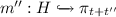
We assume a graph transformation based formalism for the definition of steps changing a graph while possibly also determining a progress of time. We abstract from the actual timed graph transformation formalism employed but only assume that it is capable to generate so-called timed graph sequences (short TGSs), which contain the graphs, their modifications, and the elapsed time between successive graphs. In the following, we are concerned with TGSs in which either only the past states of sequences are given in the form of finite TGSs or where, alternatively, an infinite TGS describes a nonterminating evolution of a system.

A step from a graph G to a graph $G'$ where G has remained unchanged for a duration of $\delta$, which may be determined by a timed graph transformation formalism, is represented by $G\cdot (\delta ,l,r)\cdot G'$ in our notion of TGSs. In this representation, the monos and identify the graph elements that are preserved from G to $G'$, i.e., $G-l( IG )$ are the nodes and edges that are present in G but are deleted to obtain $G'$ and $G'-r( IG )$ are the nodes and edges that do not exist in G but are created to obtain $G'$.¹

Definition 3

(Timed Graph Sequences (TGSs)). We inductively define the class of finite timed graph sequences (TGSs) $\varPi _{ fin }$ as follows:

• If $\pi =G_{ init }$ is the sequence containing only the graph $G_{ init }$, then .

• If $\pi \in \varPi _{ fin }$ is a TGS ending with a graph G, , are monos (for an interface graph $IG$), and is the timepoint where the graph G is changed relative to the previous change, then $\pi \cdot (\delta ,l,r)\cdot G'\in \varPi _{ fin }$.

The class of TGSs $\varPi$ contains the finite TGSs $\varPi _{ fin }$ from above and all infinite sequences that have only finite TGSs from $\varPi _{ fin }$ as prefixes.

Moreover, ${\text {dur}}(\pi )$ denotes the sum of all durations $\delta$ contained in $\pi$. Additionally, if ${\text {dur}}(\pi ) =\infty$, $\pi _t$ denotes the unique graph at time t, i.e., if $\pi =G$ then $\pi _t=G$ and if $\pi =G\cdot (\delta ,l,r)\cdot \pi '$ then ($\pi _t=G$ for $t<\delta$) and ($\pi _t=\pi '_{t-\delta }$ for $t\ge \delta$). Finally, if ${\text {dur}}(\pi ) =\infty$, $\pi _{[t_1,t_2]}$ denotes the finite TGS contained in $\pi$ between and including $\pi _{t_1}$ and $\pi _{t_2}$.

We do not require that every step modifies the current graph (i.e., we permit $G=G'$ possibly using $l=r=\mathrm {id}_{G}$). Also, time may not elapse in a step (i.e., we permit $\delta =0$) but for well-definedness of the satisfaction relation for TGSs we require that time diverges in every infinite TGS $\pi$ (i.e., ${\text {dur}}(\pi ) =\infty$).

In our running example, we simplify the presentation by using only inclusions l and r. The TGS $\pi$ given in Fig. 2 contains five graphs $G_i$ for $i \in \{0,1,2,3,4\}$ showing the system states in five different points in time, namely 0, 5, 10, 13, and 15. The corresponding durations where the respective graphs $G_i$ remain unchanged are denoted by $\delta _i$ for $i \in \{0,1,2,3\}$.

Fig. 2.

A TGS $\pi$ for our running example. For $i \in \{0,1,2,3\}$, the arrows between graphs of the TGS describe changes $G_i\cdot (\delta _i,l_i,r_i)\cdot G_{i+1}$ where the inclusions $l_i$ and $r_i$ are implicitly given by the usage of the same names in all graphs.

Fig. 3.

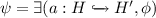
The property P from our running example formalized by the MTGC $\psi$

The syntax of MTGL is given by Metric Temporal Graph Conditions (short MTGCs) introduced in the following definition. The distinguishing feature of MTGL is the extension of the binding of graph elements used by the operator exists in GCs to the until operator of MTL. This allows for the formalization of properties where a match into a graph is preserved/extended over multiple timepoints in the subsequently introduced semantics for TGSs.

Definition 4

(Metric Temporal Graph Conditions (MTGCs)). The class of metric temporal graph conditions (MTGCs) $\varPhi ^{\mathrm {MTGC}} _H$ for the graph H contains $\psi$ if one of the following cases applies.

• $\psi =\wedge S$ and $S=\{\phi _1,\dots ,\phi _n\}\subseteq \varPhi ^{\mathrm {MTGC}} _H$.

• $\psi =\lnot \phi$ and $\phi \in \varPhi ^{\mathrm {MTGC}} _H$.

• $\psi =\exists (a, \phi )$, , and $\phi \in \varPhi ^{\mathrm {MTGC}} _{H'}$.

• $\psi =\phi _1\mathrel {{\text {U}}_{I}}\phi _2$, I is an interval over , and $\{\phi _1,\phi _2\}\subseteq \varPhi ^{\mathrm {MTGC}} _H$.

Further metric temporal operators can be defined as for MTL and GCs.

For our running example, we formalize the property P from Sect. 1 by the MTGC $\psi$ depicted in Fig. 3. In this MTGC, we additionally use the forall-new operator in the form of to match the pattern $H'$ into the considered TGS as soon as possible, i.e., precisely at the minimal timepoint, at which all elements of $H'$ exist. This operator can be encoded by the equivalent MTGC $\lnot ((\lnot \exists (a,\lnot \phi ))\mathrel {{\text {U}}_{[0,\infty )}}\exists (a,\lnot \phi ) )$, which intuitively states that “there is no violation ever that did not exist before”. Moreover, we use notational conventions to simplify our presentation of MTGCs by omitting elements in subconditions. Firstly, we omit nodes (such as $T$) if no new edges or attributes are attached to them. Secondly, we omit edges (such as $e_1$) if no new attributes are attached to them. Finally, we omit attributes (such as $id$ of $T$) in general.

The MTGC $\psi$ properly formalizes the property P using the binding capabilities of MTGL as follows: the nodes $T$, $S$, and $H$ (together with the edges $e_1$, $e_2$ as well as their attributes) are shared among the two subconditions of the until operator. This implies that the Handler node that must be matched by the right subcondition of the until operator is the previously bound Handler node $H$. Similarly, the System node that may be matched by the left subcondition of the until operator is the previously bound System node $S$.

Next we present the MTGL semantics for TGSs that defines when a given TGS satisfies a given MTGC. For the definition of this semantics, we first introduce the concept of a match that is preserved over a finite number of steps given by a finite TGS. In the following, we also call such a preserved match a binding. The preservation of the match is guaranteed by adapting it according to the renaming determined by the steps of the TGS for the case where these steps do not remove any element initially matched.

Definition 5

(Preserved Match for a Finite TGS). A mono is preserved over a finite TGS $\pi$ that starts in $G_0$ and ends in $G_n$ resulting in a mono , written , if one of the following cases applies.

• $\pi =G_0=G_n$ and $m=m'$.

• and there is such that $m=l\circ m''$ and .

The fact that the step does not remove elements that are matched by a mono m is obtained from the existence of a mono $m''$ making the triangle $m=l\circ m''$ commute. The required renaming is then performed by replacing the match m by $r\circ m''$. The mono $m''$ is uniquely defined when it exists.

Based on the preservation of matches, we now define the semantics for TGSs.

Definition 6

(Satisfaction of MTGCs by TGSs). A given MTGC $\psi \in \varPhi ^{\mathrm {MTGC}} _{H}$ is satisfied by a TGS $\pi$, an observation timepoint , and a mono , written $(\pi ,t,m)\models _{\mathrm {TGS}} \psi$, if one of the following cases applies.

• $\psi =\wedge S$ and $(\pi ,t,m)\models _{\mathrm {TGS}} \phi$ for each $\phi \in S$.

• $\psi =\lnot \phi$ and not $(\pi ,t,m)\models _{\mathrm {TGS}} \phi$.

• and there is some such that $q\circ a=m$ and $(\pi ,t,q)\models _{\mathrm {TGS}} \phi$.

• $\psi =\phi _1\mathrel {{\text {U}}_{I}}\phi _2$ and there is some $t'\in I$ such that

  • there is s.t. and $(\pi ,t+t',m')\models _{\mathrm {TGS}} \phi _2$ and

  • for every $t''\in [0,t')$ it holds that there is an such that and $(\pi ,t+t'',m'')\models _{\mathrm {TGS}} \phi _1$.

An MTGC $\psi$ over the empty graph is satisfied by a TGS $\pi$, written $\pi \models _{\mathrm {TGS}} \psi$, if $(\pi ,0,\mathrm {i}_{\pi _0})\models _{\mathrm {TGS}} \psi$ where is the initial morphism to the graph at timepoint 0 of $\pi$ (i.e., the first graph of $\pi$).

This semantics is similar to the semantics of GCs for conjunction, negation, and the exists operator since for the triple $(\pi ,t,m)$ it always holds that the codomain of m is the graph $\pi _t$ and since the checked MTGC is defined for the domain of m. The TGS $\pi$ and the current timepoint t are used in the case for the until operator where we rely on the preserved match relation from above to change the codomain of a match from $\pi _t$ to the graphs $\pi _{t+t'}$ and $\pi _{t+t''}$ at later timepoints.

Example 1

(TGS satisfies MTGC). Considering our running example, we argue that the MTGC given in Fig. 3 is satisfied by the TGS given in Fig. 2. Firstly, the forall-new operator matches the nodes T, S and the edge $e_1$ in $G_2$ at timepoint 10, which is the maximal creation timepoint of these three elements. Then, the exists operator matches the node $H$ together with the edge $e_2$ in $G_2$ at the same timepoint. Finally, the until operator matches subsequently the node $R$ and the edge $e_3$ in $G_3$ at the timepoint 13 and the remainder $true$ is trivially satisfied for the timepoint 13. In addition, as also required by the until operator, for every timepoint in the interval $[10,13)$, it is not possible to match a second Handler node $H'$ that is connected to S. This holds because the graph in $\pi$ for the timepoints in this interval is the graph $G_2$, which indeed does not contain such a second Handler node.

5 Mapping of TGSs to Graphs with History

Subsequently, we are concerned with finite TGSs $\pi$ (which have a finite number of steps and therefore also satisfy ${\text {dur}}(\pi ) <\infty$) for which the satisfaction of an MTGC $\psi$ is decidable [4] when replacing in $\psi$ right-open intervals $[r,\infty )$ and $(r,\infty )$ by $[r,{\text {dur}}(\pi ))$ and $(r,{\text {dur}}(\pi ))$, respectively. Such an adaptation of intervals leads to an MTGC $\psi '$ that is bounded and for which the satisfaction by the finite TGS $\pi$ is equivalent (i.e., $\pi \models _{\mathrm {TGS}} \psi \iff \pi \models _{\mathrm {TGS}} \psi '$).

To analyze the satisfaction of an MTGC by a given finite TGS, we now introduce the notion of graphs with history (in short, GHs) as an equivalent representation of a given finite TGS. Afterwards, we introduce a semantics operating on this alternative representation (called in the following semantics for GHs) that is compatible with the semantics introduced before for TGSs. The translation from finite TGSs to GHs reduces the size of the representation in terms of the stored data. Moreover, it decouples the observation of modifications, resulting in a GH, and the subsequent satisfaction check for possibly several MTGCs.

The notion of GHs for capturing the changes to a current graph over time as given by a TGS $\pi$, requires that the used type graph $TG$ contains for all nodes and edges the attributes ${\text {cts}}$ and ${\text {dts}}$ of sort $\mathsf {real}$ to capture the total timepoint at which an element was created and (if applicable) deleted, respectively.²

Definition 7

(Graphs with History (GHs)). Let $TG$ be a type graph where all nodes and edges have attributes ${\text {cts}}$ denoting the timepoint of their creation and ${\text {dts}}$ denoting the timepoint of their deletion. Then $G_H$ is a graph with history (GH) if it is typed over $TG$ satisfying the following consistency requirements.³

• There is precisely one ${\text {cts}}$ attribute for every graph node and edge.

• There is at most one ${\text {dts}}$ attribute for every graph node and edge.

• For an edge e, the value of the ${\text {cts}}$ attributes of the source and the target nodes of e are less or equal to the ${\text {cts}}$ attribute of e.

• For an edge e, the value of the ${\text {dts}}$ attributes of the source and the target nodes of e are greater or equal to the ${\text {dts}}$ attribute of e.

We now define the operation , which converts a finite TGS $\pi$ (i.e., a TGS with a finite number of steps) into the corresponding GH $G_H$. This recursive operation handles the renaming given by the monos l and r in the steps of $\pi$ and, moreover, encodes the insertion of additional nodes/edges $\alpha$ by adding attributes ${\text {cts}} =t$ for these nodes/edges in the constructed $G_H$ and by equipping removed nodes/edges $\alpha$ with an additional attribute ${\text {dts}} =t$ where t is the current total time of the considered TGS $\pi$ in both cases.

Definition 8

(Map TGS to GH (Operation )).

• If $\pi =G_{ init }$, then is obtained from $G_{ init }$ by adding the attributes ${\text {cts}} (\alpha )=0$ to each node or edge $\alpha$ in $G_{ init }$.

• If is a TGS, is the GH obtained from the mapping of the TGS $\pi '$ using the operation , and $t={\text {dur}}(\pi ')$ is the total time of $G_H'$, then is constructed from $G_H'$ by adding the attributes ${\text {dts}} (\alpha )=t+\delta$ to each node or edge $\alpha \in G-l( IG )$, by renaming each node and edge $\alpha \in l( IG )$ according to l, by adding each node and edge $\alpha \in G'-r( IG )$, by renaming each node and edge $\alpha \in r( IG )$ according to r, and by adding the attributes ${\text {cts}} (\alpha )=t+\delta$ to each node or edge $\alpha \in G'-r( IG )$.

The following example covers an application of to a finite TGS.

Example 2

(Map TGS to GH). We map the finite TGS $\pi$ from Fig. 2 to the GH $G_H$ shown in Fig. 4 using the operation as follows. Since $\pi$ starts with an empty graph $G_0$, we first map it into the empty GH. The second state of $\pi$ given by $G_1$ including the System node S is added to the TGS after 5 timeunits. We map this TGS state to the GH by adding S to the empty GH and by, additionally, equipping this node with the creation timepoint ${\text {cts}} =5$. After another 5 timeunits, an additional Task node T, a Handler node H, and edges $e_1$, $e_2$ between the existing System node S and the new Task node T resp. the new Handler node H are added to the TGS resulting in the TGS state $G_2$. These changes are again mapped to the GH by adding the Task node T, the Handler node H, and the edges $e_1$, $e_2$ to the current version of $G_H$ as well as by additionally equipping them with the creation timepoints ${\text {cts}} =10$. In a similar manner the Result node R together with the edges $e_3$ and $e_4$ (see the TGS state $G_3$) are added to the GH with the creation timepoints ${\text {cts}} =13$. Finally, after 2 timeunits, the edge $e_3$ is deleted to obtain the TGS state $G_4$. To reflect this in the GH, we add to the edge $e_3$ in $G_H$ the additional deletion timepoint ${\text {dts}} =15$.

Fig. 4.

Mapping of the TGS $\pi$ from Fig. 2 to the GH

For the satisfaction of an MTGC of the form , where the exists operator is inherited from GCs, it is still required that the pattern that is found so far (given by some mono ) in the host graph $G_H$ can be extended to a larger pattern (given by some mono ). Additionally, we have to check that all matched elements are already created (because the GH also contains the elements created with higher ${\text {cts}}$ values) but not yet deleted (because the GH also contains the elements deleted at earlier timepoints). For the satisfaction of an MTGC of the form $\phi _1\mathrel {{\text {U}}_{I}}\phi _2$, where the until operator is inherited from MTL, it is still required that $\phi _2$ must be satisfied at some timepoint $t'$ in the interval I relative to the current observation timepoint t and that $\phi _1$ is continuously satisfied (by a possibly varying match for each timepoint) for all timepoints preceding $t'$.

Definition 9

(Satisfaction of MTGCs by GHs). An MTGC $\psi \in \varPhi ^{\mathrm {MTGC}} _{H}$ is satisfied by a mono and an observation timepoint , written $(m,t)\models _{\mathrm {GH}} \psi$, if $\max (\{0\}\cup {\text {cts}} (m(H)))\le t<\min (\{\infty \}\cup {\text {dts}} (m(H)))$ and one of the following cases applies.

• $\psi =\wedge \{\phi _1,\dots ,\phi _n\}$ and $(m,t)\models _{\mathrm {GH}} \phi _i$ (for all $1\le i\le n$).

• $\psi =\lnot \phi$ and not $(m,t)\models _{\mathrm {GH}} \phi$.

• and there is some such that $q\circ a=m$ and $(q,t)\models _{\mathrm {GH}} \phi$.

• $\psi =\phi _1\mathrel {{\text {U}}_{I}}\phi _2$ and there is some $t'\in I$ such that $(m,t+t')\models _{\mathrm {GH}} \phi _2$ and for every $t''\in [0,t')$ it holds that $(m,t+t'')\models _{\mathrm {GH}} \phi _1$.

An MTGC $\psi$ over the empty graph is satisfied by a GH $G_H$, written $G_H\models _{\mathrm {GH}} \psi$, if $(\mathrm {i}_{G_H},0)\models _{\mathrm {GH}} \psi$ where is the initial morphism to $G_H$.

Note that the reasoning for the satisfaction of the MTGC $\psi$ from Fig. 3 by from Fig. 4 proceeds analogously to Example 1.

In the following theorem (see [11] for its proof), we state the compatibility of the two satisfaction relations for the case of finite TGSs showing that they can be used interchangeably to determine the satisfaction of an MTGC in this case.

Theorem 1

(Soundness of Operation ). If $\pi \in \varPi _{ fin }$ and $\psi \in \varPhi ^{\mathrm {MTGC}} _{\emptyset }$ then $\pi \models _{\mathrm {TGS}} \psi$ iff .

6 Reduction of MTGL to GCs

We now introduce a procedure for checking the satisfaction of an MTGC by a GH using a reduction of an MTGC to a corresponding GC. Based on the operation from the previous section, we thereby obtain a checking procedure for finite TGSs as well. Moreover, this reduction shows that MTGL is as expressive as the logic of GCs on finite TGSs (since every GC is trivially also an MTGC).

Fig. 5.

The GC $\psi '$ and the adapted graph $G_H'$ resulting from applying the operation to the GH from Fig. 4, the timepoint $t=10$, and the MTGC $\psi$ from Fig. 3 (where the outermost $forall-new$ operator has been simplified to the $forall$ operator)

We first present the operation for translating an MTGC into the corresponding GC and then show that this translation (also called reduction in the following) is compatible with our semantics for GHs and the operation from before. The operation encodes in the resulting GC all parts of the satisfaction relation $\models _{\mathrm {GH}}$ that are not covered by the satisfaction relation $\models$ for GCs. In particular, the operation removes all occurrences of the until operator and encodes the check that the elements that are matched by the exists operator have all been created as well as that none of them has yet been deleted.

Technically, we translate a GH for a finite TGS $\pi$, $\psi \in \varPhi ^{\mathrm {MTGC}} _{\emptyset }$, and an observation timepoint (where $G_H$ and $\psi$ are typed over a type graph $TG$) into a graph $G_H'$ and $\psi '\in \varPhi ^{\mathrm {GC}} _{\emptyset }$ (where both are typed over a changed type graph $TG '$) using the procedure presented in Definition 10. We obtain $\psi '$ from $\psi$ by encoding the until operator suitably and by implementing the checks of ${\text {cts}}$ and ${\text {dts}}$ attributes according to Definition 9 for the exists and until operators using attribute constraints, for which we add variables to $\psi$. We also add the same variables to $G_H$ to obtain $G'_H$.

Definition 10

(Reduce MTGC to GC (Operation )). The recursive operation takes 3 arguments:  a GH $G_H$ that has been obtained by application of the operation to a TGS  $\pi$, an observation timepoint , and an MTGC $\psi \in \varPhi ^{\mathrm {MTGC}} _{\emptyset }$. $G_H$ and all graphs contained in $\psi$ are typed over the type graph $TG$.

The operation returns a pair $(G_H',\psi ')$ consisting of a graph $G_H'$ (which is a slight modification of $G_H$) and a GC $\psi '\in \varPhi ^{\mathrm {GC}} _{\emptyset }$. The graph $G_H'$ and all graphs contained in $\psi '$ are typed over an adapted type graph $TG'$ (called a reduction type graph) introduced below.

• 1. (Construction of the reduction type graph $TG'$):

  We adapt the original type graph $TG$ to $TG '$ by adding an $\text {Encoding}$ node with attributes $\mathrm {num}:\mathsf {int}$ and $\mathrm {var}:\mathsf {real}$.

• 2. (Construction of the MTGC $\psi _{att}$ with ${\text {cts}}$ and ${\text {dts}}$ attributes):

  We obtain $\psi _{ att }$ from $\psi$ by adding the attributes ${\text {cts}} =x_{c,\alpha }$ and ${\text {dts}} =x_{d,\alpha }$ to all nodes and edges $\alpha$ contained in graphs in $\psi$.

• 3. (Construction of the GC $\psi '$):

  where $G_0$ is the graph containing the $\text {Encoding}$ node $v_0$ with the attributes $\mathrm {num}\,=\, 0$, $\mathrm {var}\,=\, x_{0}$ as well as the attribute constraint $x_0=t$ and is the initial morphism to $G_0$. Then, if one of the following cases applies (where $\psi _{att}$ is the condition to be reduced, $x_o$ is the timepoint at which the subcondition must be satisfied, $G_a$ is the graph containing additional nodes, edges, and attribute constraints to be added to the graphs in conditions constructed, and G is the graph over which the condition $\psi _{att}$ is defined).

  • (a) $\psi _{att}=\wedge S$ and .

  • (b) $\psi _{att}=\lnot \phi$ and .

  • (c) and where $G_a'$ equals the graph $G_a$, to which an $\text {Encoding}$ node $v_{n}$ with the attributes $\mathrm {num}\,=\, n$, $\mathrm {var}\,=\, x_n$ (where no $\text {Encoding}$ node has been created in the reduction for n so far) and the attribute constraint $x_n=x_o$ have been added, $H_1'=G_a\cup H_1$, $H_2'=G_a'\cup H_2$, $H_3'$ equals the graph $H_2'$, to which the attribute constraints $\lnot {\mathrm {alive}}({x_n},{H_2})$ have been added,⁴ $a'$ is obtained as the union of a and the identity morphism $\mathrm {id}_{G_a}$, and m is an inclusion.

  • (d) $\psi _{att}=\phi _1\mathrel {{\text {U}}_{I}}\phi _2$ and where $G_a'$ equals the graph $G_a$, to which an $\text {Encoding}$ node $v_{n_1}$ with the attributes $\mathrm {num}\,=\, n_1$, $\mathrm {var}\,=\, x_{n_1}$ (where no $\text {Encoding}$ node has been created in the reduction for $n_1$ so far) and the attribute constraints equivalent to $x_{n_1}\in I$ have been added, $G_0=G\cup G_a$, $G_1=G\cup G_a'$, $m_0$ is an inclusion, $G_a''$ equals the graph $G_a'$, to which an $\text {Encoding}$ node $v_{n_2}$ with the attributes $\mathrm {num}\,=\, n_2$, $\mathrm {var}\,=\, x_{n_2}$ (where no $\text {Encoding}$ node has been created in the reduction for $n_2$ so far) and the attribute constraints equivalent to $x_{n_2}\in [x_o,x_o+x_{n_1})$ have been added, $G_2=G_1\cup G_a''$, and $m_1$ is an inclusion.

• 4. (Construction of the graph $G_H'$):

  We obtain $G_H'$ by adding elements to $G_H$ as follows:

  • (a) We add the attribute ${\text {dts}} =-1$ to all nodes/edges without that attribute.

  • (b) We insert all $\text {Encoding}$ nodes contained in graphs in $\psi '$ together with their $\mathrm {num}\,=\, n$ and $\mathrm {var}\,=\, x_n$ attributes.

  • (c) We add the attribute constraints added during the reduction except for the $\mathrm {alive}$ constraints.

We now demonstrate how the operation can be applied to the MTGC from our running example.

Example 3

(Reduce MTGC to GC). We now apply the operation to GH from Fig. 4, the timepoint $t=10$, and the MTGC $\psi$ from Fig. 3 resulting in $G_H'$ and $\psi '$ given in Fig. 5. However, to simplify the presentation, we replaced the enclosing forall-new operator by the forall operator to avoid the substitution of the forall-new operator by its encoding from Sect. 4.

• 1. We add the attribute $\mathrm {{\text {dts}}}\,=\, x_{d,\alpha }$ to all nodes/edges $\alpha$ of $G_H$ without ${\text {dts}}$ attribute and add the attribute constraint $x_{d,\alpha }=-1$ to the set of constraints. With these additional attributes and the $\mathrm {{\text {cts}}}\,=\, x_{c,\alpha }$ attributes introduced by the operation , we are able to state the existence of nodes/edges at a given timepoint $x_n$ using attribute constraints in the resulting GC $\psi '$.

• 2. We add a unique Encoding node to each graph in $\psi '$ as a container for additional variables $x_n$ that are used in attribute constraints to encode the current observation timepoint (the num attributes are included to decrease the number of matches to be considered). Initially, we add an enclosing exists operator with the attribute constraint $x_{0}=t$ (see $\varTheta _0$) where t is the input observation timepoint that is 10 for this application of . Further attribute constraints then relate the additional variables $x_n$ for existential/universal quantifications (see $\varTheta _1$, $\varTheta _2$, $\varTheta _4$, and $\varTheta _6$). For the encoding of the until operator, these observation timepoints ($x_3$ in $\varTheta _3$ and $x_5$ in $\varTheta _5$) are restricted to some interval as described below.

• 3. We encode the exists operator for the MTGC $\phi$ according to Definition 9 using an additional negative graph condition stating that the matched nodes/edges $\alpha$ are not violating the attribute constraints in $\text {alive}({x_n},{\alpha })$. The set $\text {alive}({x_n},{\alpha })$ contains the constraint $x_n\le x_{c,\alpha }$ (to state that $\alpha$ was created before $x_n$) and the constraint $x_{d,\alpha }=-1\vee x_n<x_{d,\alpha }$ (to state that $\alpha$ was not deleted or that it is deleted later than $x_n$).

• 4. We encode the until operator $\phi _1\mathrel {{\text {U}}_{I}}\phi _2$ for the MTGCs $\phi _1$ and $\phi _2$ according to Definition 9 using the exists operator (the forall operator used in the GC below is only an abbreviation for a usage of the exists operator according to Definition 1). Informally, $\phi _1\mathrel {{\text {U}}_{[t_1,t_2]}}\phi _2$ (the construction is similar for other kinds of intervals) is equivalent to $\exists (t'\in [x_n+t_1,x_n+t_2],\phi '_2\wedge \forall (t''\in [x_n+t_1,t'),\phi '_1))$ where $\phi _1'$ and $\phi _2'$ are the reductions of $\phi _1$ and $\phi _2$, respectively. The variable $x_n$ refers to the current observation timepoint that depends on the timepoint where an enclosing condition has been matched. In the example, the variables $x_n$, $t'$, and $t''$ are represented in $\psi '$ by the variables $x_2$, $x_3$, and $x_5$, respectively. The reduction is recursively applied to $\phi _1$ and $\phi _2$ resulting in $\phi _1'$ and $\phi _2'$, respectively. The replacement GC for the until subcondition spans the last four lines of $\psi '$ in Fig. 5.

• 5. We add all Encoding nodes occurring in $\psi '$ to $G_H$ as depicted in Fig. 5. The Encoding nodes are used in $\psi '$ as containers for the additional variables employed in the attribute constraints and are required in $G_H'$ to allow for matchings from the adapted graphs of $\psi '$ to $G_H'$.

In the following theorem (see [11] for its proof), we state that the operation is sound w.r.t. the satisfaction relations for MTGCs and GCs.

Theorem 2

(Soundness of Operation ). If $\pi \in \varPi _{ fin }$, , $\psi \in \varPhi ^{\mathrm {MTGC}} _{\emptyset }$, is a timepoint, is the initial morphism to $G_H$, and , then $(\mathrm {i}_{G_H},t)\models _{\mathrm {GH}} \psi$ iff $G_H'\models \psi '$.

By application of Theorem 2, we can deduce for our running example that the MTGC $\psi$ from Fig. 3 translated by the operation is satisfied by the graph $G'_H$ (both given in Fig. 5). For this purpose observe that $\psi$ from Fig. 3 (simplified as stated in Fig. 5) is satisfied by the GH from Fig. 4 for the timepoint $t=10$ since the unique match of the Task node $T$, the on edge $e_1$, and the System node $S$ satisfies the remaining condition starting at timepoint $t=10$.

7 Tool Support

We provide tool support for checking finite TGSs against MTGCs as an extension of $\textsc {AutoGraph}$  [25]. Firstly, we extended the support of $\textsc {AutoGraph}$ to handle TGSs and MTGCs. Secondly, we implemented the operation from Definition 8 to consolidate a TGS $\pi$ to a GH $G_H$. Thirdly, we implemented the operation from Definition 10 to reduce an MTGC $\psi$ to a GC $\psi '$ and to adapt $G_H$ to a graph $G_H'$. On the foundation of these three steps and as applications of our theoretical results (see Theorems 1 and 2), we then use the built-in support of $\textsc {AutoGraph}$ for checking whether the obtained graph $G_H'$ satisfies the reduced GC $\psi '$. Note that $\textsc {AutoGraph}$ depends in this scenario on the constraint solver Z3 [20] to check satisfiability of expressions involving the values of ${\text {cts}}$ and ${\text {dts}}$ attributes of sort $\mathsf {real}$ as well as the additional constraints introduced by that contain further variables of sort $\mathsf {real}$.

Considering our running example, we observed negligible runtime and memory consumption when verifying that the finite TGS $\pi$ from Fig. 2 satisfies the MTGC $\psi$ from Fig. 3 using our implementation due to the short length of $\pi$. Overall, the application of the $\textsc {AutoGraph}$ extension to our running example shows promising results albeit the potential of further improvements regarding efficiency for handling more elaborate problem instances.

8 Conclusion and Future Work

We defined Metric Temporal Graph Logic (MTGL) by integrating the metric temporal operator until with time bounds into the well-established logic of (nested) graph conditions (GCs). This new logic allows to maintain an established binding of graph elements throughout the analysis of a timed sequence of (typed attributed) graphs (TGSs). Furthermore, to enable a satisfaction check for MTGL conditions by finite TGSs, we introduced a mapping of a finite TGS $\pi$ into a graph with history and defined a reduction of an MTGL condition $\psi$ to a GC $\psi '$ given by where the graph with history $G_H$ is extended to a graph $G_H'$. For this mapping and this reduction, we have proven that the satisfaction checks for the different representations are consistent (i.e., $\pi \models _{\mathrm {TGS}} \psi \iff G_H\models _{\mathrm {GH}} \psi \iff G_H'\models \psi '$). Finally, we presented an extension of the tool $\textsc {AutoGraph}$ allowing to check the satisfaction of MTGL conditions by finite TGSs via the introduced mapping and reduction.

In the future, we want to develop checking procedures bounded MTGL conditions such that only violations that hold for any possible continuation are reported. Moreover, we intend to use our reduction of MTGL conditions to related GC counterparts for invariant checking for graph transformation systems as considered in [7]. Furthermore, we want to develop extensions of MTGL that include branching such as in timed CTL, that are applicable to the setting of probabilistic timed graph transformation systems as introduced in [19], or that support additional features e.g. permitting variables in the interval bounds of MTGL conditions or in attribute constraints. Finally, we intend to develop a model checking procedure for MTGL and these extensions. Besides these technical advancements we intend to evaluate and compare our approach based on benchmarks from applications domains such as runtime monitoring [18].

References

Arendt, T., Biermann, E., Jurack, S., Krause, C., Taentzer, G.: Henshin: advanced concepts and tools for in-place EMF model transformations. In: Petriu, D.C., Rouquette, N., Haugen, Ø. (eds.) MODELS 2010. LNCS, vol. 6394, pp. 121–135. Springer, Heidelberg (2010). https://doi.org/10.1007/978-3-642-16145-2_9
Baldan, P., Corradini, A., König, B.: A framework for the verification of infinite-state graph transformation systems. Inf. Comput. 206(7), 869–907 (2008). https://doi.org/10.1016/j.ic.2008.04.002
Basin, D., Klaedtke, F., Müller, S., Zălinescu, E.: Monitoring metric first-order temporal properties. J. ACM (JACM) 62(2), 15 (2015). http://dl.acm.org/citation.cfm?id=2699444
Bouyer, P., Markey, N., Ouaknine, J., Worrell, J.: The cost of punctuality. In: LICS 2007, pp. 109–120. IEEE Computer Society (2007). https://doi.org/10.1109/LICS.2007.49
Courcelle, B.: The expression of graph properties and graph transformations in monadic second-order logic. In: Handbook of Graph Grammars, pp. 313–400. World Scientific (1997). ISBN 9810228848
Dávid, I., Ráth, I., Varró, D.: Foundations for streaming model transformations by complex event processing. Softw. Syst. Model. 17(1), 135–162 (2018). https://doi.org/10.1007/s10270-016-0533-1
Dyck, J., Giese, H.: k-inductive invariant checking for graph transformation systems. In: de Lara, J., Plump, D. (eds.) ICGT 2017. LNCS, vol. 10373, pp. 142–158. Springer, Cham (2017). https://doi.org/10.1007/978-3-319-61470-0_9
The Eclipse Foundation: EMF Henshin (2013). http://www.eclipse.org/modeling/emft/henshin
Ehrig, H., Ehrig, K., Prange, U., Taentzer, G.: Fundamentals of Algebraic Graph Transformation. Springer, Heidelberg (2006). https://doi.org/10.1007/3-540-31188-2
Ghamarian, A.H., de Mol, M., Rensink, A., Zambon, E., Zimakova, M.: Modelling and analysis using GROOVE. STTT 14(1), 15–40 (2012). https://doi.org/10.1007/s10009-011-0186-x
Giese, H., Maximova, M., Sakizloglou, L., Schneider, S.: Metric temporal graph logic over typed attributed graphs: An extended version. Technical report, 127, Hasso Plattner Institute at the University of Potsdam, Potsdam, Germany (2019)
Habel, A., Pennemann, K.H.: Correctness of high-level transformation systems relative to nested conditions. Math. Struct. Comput. Sci. 19, 1–52 (2009). https://doi.org/10.1017/S0960129508007202
Jakumeit, E., et al.: A survey and comparison of transformation tools based on the transformation tool contest. Sci. Comput. Program. 85, 41–99 (2014). https://doi.org/10.1016/j.scico.2013.10.009
Klein, F., Giese, H.: Joint structural and temporal property specification using timed story scenario diagrams. In: Dwyer, M.B., Lopes, A. (eds.) FASE 2007. LNCS, vol. 4422, pp. 185–199. Springer, Heidelberg (2007). https://doi.org/10.1007/978-3-540-71289-3_16
König, B., Kozioura, V.: Augur 2—a new version of a tool for the analysis of graph transformation systems. ENTCS 211, 201–210 (2008). https://doi.org/10.1016/j.entcs.2008.04.042
Koymans, R.: Specifying real-time properties with metric temporal logic. Real-Time Syst. 2(4), 255–299 (1990). http://www.springerlink.com/index/X37127R758453X73.pdf
Kwiatkowska, M., Norman, G., Parker, D.: PRISM 4.0: verification of probabilistic real-time systems. In: Gopalakrishnan, G., Qadeer, S. (eds.) CAV 2011. LNCS, vol. 6806, pp. 585–591. Springer, Heidelberg (2011). https://doi.org/10.1007/978-3-642-22110-1_47
Leucker, M., Schallhart, C.: A brief account of runtime verification. J. Log. Algebr. Program. 78(5), 293–303 (2009). https://doi.org/10.1016/j.jlap.2008.08.004
Maximova, M., Giese, H., Krause, C.: Probabilistic timed graph transformation systems. In: de Lara, J., Plump, D. (eds.) ICGT 2017. LNCS, vol. 10373, pp. 159–175. Springer, Cham (2017). https://doi.org/10.1007/978-3-319-61470-0_10
Microsoft Corporation: Z3. https://github.com/Z3Prover/z3. Accessed 19 Sept 2017
Orejas, F.: Symbolic graphs for attributed graph constraints. J. Symb. Comput. 46(3), 294–315 (2011). https://doi.org/10.1016/j.jsc.2010.09.009
Ouaknine, J., Worrell, J.: Some recent results in metric temporal logic. In: Cassez, F., Jard, C. (eds.) FORMATS 2008. LNCS, vol. 5215, pp. 1–13. Springer, Heidelberg (2008). https://doi.org/10.1007/978-3-540-85778-5_1
Pennemann, K.H.: Development of correct graph transformation systems, Ph.D. thesis, Dep. Informatik, Univ. Oldenburg (2009)
Rensink, A.: Representing first-order logic using graphs. In: Ehrig, H., Engels, G., Parisi-Presicce, F., Rozenberg, G. (eds.) ICGT 2004. LNCS, vol. 3256, pp. 319–335. Springer, Heidelberg (2004). https://doi.org/10.1007/978-3-540-30203-2_23
Schneider, S., Lambers, L., Orejas, F.: Automated reasoning for attributed graph properties. STTT 20(6), 705–737 (2018). https://doi.org/10.1007/s10009-018-0496-3
University of Twente: Graphs for Object-Oriented Verification (GROOVE) (2011). http://groove.cs.utwente.nl
Author information
Authors and Affiliations
Corresponding author
Editor information
Editors and Affiliations
Rights and permissions
Open Access This chapter is licensed under the terms of the Creative Commons Attribution 4.0 International License (http://creativecommons.org/licenses/by/4.0/), which permits use, sharing, adaptation, distribution and reproduction in any medium or format, as long as you give appropriate credit to the original author(s) and the source, provide a link to the Creative Commons license and indicate if changes were made.
The images or other third party material in this chapter are included in the chapter's Creative Commons license, unless indicated otherwise in a credit line to the material. If material is not included in the chapter's Creative Commons license and your intended use is not permitted by statutory regulation or exceeds the permitted use, you will need to obtain permission directly from the copyright holder.
Copyright information
© 2019 The Author(s)
About this paper
Cite this paper
Giese, H., Maximova, M., Sakizloglou, L., Schneider, S. (2019). Metric Temporal Graph Logic over Typed Attributed Graphs. In: Hähnle, R., van der Aalst, W. (eds) Fundamental Approaches to Software Engineering. FASE 2019. Lecture Notes in Computer Science(), vol 11424. Springer, Cham. https://doi.org/10.1007/978-3-030-16722-6_16
Download citation
DOI: https://doi.org/10.1007/978-3-030-16722-6_16
Published:
Publisher Name: Springer, Cham
Print ISBN: 978-3-030-16721-9
Online ISBN: 978-3-030-16722-6
eBook Packages: Computer ScienceComputer Science (R0)