Geometry-dependent reduced-order models for the computation of homogenized transfer properties in porous media

Abstract

This article investigates reduced-order models (ROMs) based on proper orthogonal decomposition for efficient computation of the homogenized diffusion properties of saturated porous media. The homogenized tensor, whose classical expression may be obtained from periodic homogenization techniques, is computed by solving a local problem on an elementary cell that includes one or several circular solid inclusions. The cost of the repeated resolution of this problem by the finite element method for different inclusions radii may be important, and classical model order reduction methods based on the computation of a spatial basis cannot be applied directly. The method proposed in this work to cope with the variability of circular inclusions relies on the introduction of a transformation from a reference domain to the physical domain that admits an exact affine decomposition in the three-dimensional cases, allowing to split the problem into an offline learning phase and an online evaluation phase which does not depend on the number of degrees of freedom of the original full-order solution. Approximate affine decomposition for two-dimensional cases is also provided with an explicit estimation of the truncation error. The efficiency of the proposed algorithm in terms of accuracy and of computing time is evaluated first for 2D and 3D isotropic and anisotropic elementary cells with a single inclusion, and second for a 2D anisotropic cell with multiple inclusions. Furthermore the ROM is used to estimate in quasi-real time the homogenized diffusion tensor for a given probability distribution of the geometry parameters.

Appendices

Recalls on the proper orthogonal decomposition (POD)

Reduced-order models consist in approximating the solution ${\varvec{\chi }}_{\mathrm {\star }}({\varvec{\xi }}; \rho )$ of a given problem parametrized by $\rho$ on a spatial basis $\left( {\varvec{\phi }}_i\right) _{i=1}^{N_{\mathrm {rom}}}$ of small size $N_{\mathrm {rom}}$:

$$\begin{aligned} {\varvec{\chi }}_{\mathrm {\star }}({\varvec{\xi }}; \rho ) \simeq {\widehat{{\varvec{\chi }}}}_{\mathrm {\star }}({\varvec{\xi }}; \rho ) = \sum _{i=1}^{n_{\varvec{\chi }}}a_i(\rho )\,{\varvec{\phi }}_i({\varvec{\xi }}), \end{aligned}$$

where ${\varvec{\xi }}$ is the space variable. There exist numerous methods to build this spatial basis, but the most used stays the proper orthogonal decomposition that combines accuracy and optimality. The space-dependent functions ${\varvec{\phi }}_i$ obtained by the POD, lying in the Hilbert space $\big (V_{\mathrm {\star }}\big )^d$, satisfy the two conditions:

• (i) Orthogonality: $({\varvec{\phi }}_i)_i$ is orthogonal,

• (ii) Optimality of $({\varvec{\phi }}_i)_i$:

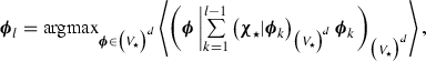
where $(\bullet \vert \bullet )_{\big (V_{\mathrm {\star }}\big )^d}$ denotes the scalar product of $\big (V_{\mathrm {\star }}\big )^d$ and $\langle \bullet \rangle$ denotes the mean over the variable $\rho$. The latter condition ensures that the space engendered by the $\{{\varvec{\phi }}_i\}_{i=1}^l$ gives the best approximation of the functions ${\varvec{\chi }}_{\mathrm {\star }}({\varvec{\xi }}; \rho )$, among the subspaces of $\big (V_{\mathrm {\star }}\big )^d$ with rank l.

The method of snapshots introduced in [33] is used in this article. It consists in computing by the FEM a set of vector fields ${\varvec{\chi }}_{\mathrm {\star }}({\varvec{\xi }}; \rho ^j)$ (called the snapshots) for a finite set of parameter values $\{\rho ^j\}_{j=1}^{N_{\mathrm {snap}}}$. Then, POD modes ${\varvec{\phi }}_i$ are sought inside the functional space $[{\varvec{\chi }}_{\mathrm {\star }}({\varvec{\xi }}; \rho ^j)]_{j=1}^{N_{\mathrm {snap}}}$. The snapshots ${\varvec{\chi }}_{\mathrm {\star }}({\varvec{\xi }}; \rho ^j)$ are expected to be linearly independent in practical cases so that, by exploiting the orthogonality and optimality conditions, the POD modes can be determined by the formula

$$\begin{aligned} {\varvec{\phi }}_i=\frac{1}{\sqrt{\lambda _i}}\sum \limits _{j=1}^{N_{\mathrm {snap}}}[{\varvec{v}}_i]_j{\varvec{\chi }}_{\mathrm {\star }}({\varvec{\xi }}; \rho ^j)\text {,} \end{aligned}$$

where $\lambda _i$ are the eigenvalues and ${\varvec{v}}_i$ are the unit eigenvectors of the symmetric positive definite correlation matrix ${\varvec{C}}$ whose coefficients are given by

$$\begin{aligned} {\varvec{C}}_{jk}=\dfrac{1}{N_{\mathrm {snap}}}\displaystyle \int \limits _{\varOmega } {\varvec{\chi }}_{\mathrm {\star }}({\varvec{\xi }}; \rho ^k)\cdot {\varvec{\chi }}_{\mathrm {\star }}({\varvec{\xi }}; \rho ^j)\text {d}{\mathbf {y}}\text {.} \end{aligned}$$

The POD basis is then truncated to a number of $N_{\mathrm {rom}}$ modes which is selected to ensure that the error on the relative content of information due to the projection on the retained POD modes is below a given threshold $\nu$:

$$\begin{aligned} N_{\mathrm {rom}}=\min \left\{ N\in 1\dots N_{\mathrm {snap}}; \;\frac{\sum \nolimits _{i=1}^N\lambda _i}{\sum \nolimits _{i=1}^{N_{\mathrm {snap}}}\lambda _i} >1-\nu \right\} \cdot \end{aligned}$$

(69)

Formulas and proofs associated with the parametrized transformation

Let us recall the definition of the transformation ${\varvec{\tau }}_\rho$, for each ${\varvec{\xi }}$ in the reference fluid domain:

$$\begin{aligned} {\varvec{\tau }}_\rho ({\varvec{\xi }}) = \left\{ \begin{array}{ll} \alpha _{\rho }{\varvec{u}}({\varvec{\xi }})+\beta _{\rho }{\varvec{\xi }}, &{}\quad \text{ if }\;\rho _{\mathrm {\star }}\le \parallel {\varvec{\xi }} \parallel < q, \\ {\varvec{\xi }},&{}\quad \text{ if }\; q\le \parallel {\varvec{\xi }} \parallel , \end{array} \right. \end{aligned}$$

where $\rho _{\mathrm {\star }}$ and $q$ are the internal and external radii of the crown ${\varOmega ^{\mathrm {\star }}_{\mathrm {c}}}$, ${\varvec{u}}({\varvec{\xi }})=\dfrac{{\varvec{\xi }}}{\parallel {\varvec{\xi }} \parallel }$ denotes the radial unit vector and

$$\begin{aligned} \alpha _{\rho }=q\dfrac{\rho -\rho _{\mathrm {\star }}}{q-\rho _{\mathrm {\star }}}, \quad \beta _{\rho }=\dfrac{q-\rho }{q-\rho _{\mathrm {\star }}}. \end{aligned}$$

The following formulas related to the Jacobian matrix of the transformation ${\varvec{\tau }}_\rho$ are the core of the affine dependence to the geometry of the proposed POD-ROM.

Lemma 1

For all $\rho$ such that $\rho < q$:

$$\begin{aligned} {\varvec{J}}_{\rho }({\varvec{\xi }})= & {} \beta _{\rho }{\varvec{I}}+\alpha _{\rho }\nabla _{\!{\varvec{\xi }}}{\varvec{u}}({\varvec{\xi }}), \end{aligned}$$

(70)

$$\begin{aligned} {\varvec{J}}_{\rho }^{-1}({\varvec{\xi }})= & {} \frac{1}{\beta _{\rho }} {\varvec{I}}-\frac{\alpha _{\rho }}{\beta _{\rho }}\cdot \frac{1}{\beta _{\rho }\Vert {\varvec{\xi }}\Vert +\alpha _{\rho }}{\varvec{G}}_{{\varvec{u}}({\varvec{\xi }})}, \end{aligned}$$

(71)

$$\begin{aligned} j_{\rho }({\varvec{\xi }})= & {} \beta _{\rho }\sum \limits _{p=0}^{d-1}C_{d-1}^p\frac{\alpha _{\rho }^p}{\Vert {\varvec{\xi }}\Vert ^p}\beta _{\rho }^{d-1-p}, \end{aligned}$$

(72)

with the convention

$$\begin{aligned} {\varvec{G}}_{{\varvec{u}}({\varvec{\xi }})} : = {\varvec{I}}-\frac{1}{\Vert {\varvec{\xi }}\Vert ^2}{\varvec{\xi }}\cdot {\varvec{\xi }}^\intercal \cdot \end{aligned}$$

(73)

Proof

(70) is obvious, it follows from the definition of ${\varvec{\tau }}_\rho$ and the linearity of the gradient operator. To prove (71) we need an explicit formula for the inverse mapping ${{\varvec{\tau }}_\rho }^{-1}$. We first notice that, according to the geometrical characterization of ${\varvec{\tau }}_\rho$ at the beginning of Sect. 3, ${{\varvec{\tau }}_\rho }^{-1}$ is obtained by switching $\rho _{\mathrm {\star }}$ and $\rho$ in ${\varvec{\tau }}_\rho$. Then we have for ${\varvec{y}}={\varvec{\tau }}_\rho ({\varvec{\xi }})$:

$$\begin{aligned} {{\varvec{\tau }}_\rho }^{-1}({\varvec{y}}) = \left\{ \begin{array}{ll} \alpha _{\rho }'{\varvec{u}}({\varvec{y}})+\beta _{\rho }' {\varvec{y}}, &{} \text{ if }\;\rho _{\mathrm {\star }}\le \parallel {\varvec{y}} \parallel < q, \\ {\varvec{y}},&{} \text{ if }\; q\le \parallel {\varvec{y}} \parallel , \end{array} \right. \end{aligned}$$

where

$$\begin{aligned} \alpha _{\rho }'=q\dfrac{\rho _{\mathrm {\star }}-\rho }{q-\rho }, \quad \beta _{\rho }'=\dfrac{q-\rho _{\mathrm {\star }}}{q-\rho }. \end{aligned}$$

Note that $\alpha _{\rho }' =-\frac{\alpha _{\rho }}{\beta _{\rho }}$ and $\beta _{\rho }'=\frac{1}{\beta _{\rho }}$. Now, differentiating ${{\varvec{\tau }}_\rho }^{-1}$ at ${\varvec{\tau }}_\rho ({\varvec{\xi }})$ to compute ${\varvec{J}}_{\rho }^{-1}({\varvec{\xi }})$ for each ${\varvec{\xi }}<q$ yields ${\varvec{J}}_{\rho }^{-1}({\varvec{\xi }})=\left( \nabla _{{\varvec{\tau }}_\rho ({\varvec{\xi }})}{{\varvec{\tau }}_\rho }^{-1}\right) ({\varvec{\tau }}_\rho ({\varvec{\xi }}))$, from which it follows by linearity that

$$\begin{aligned}{\varvec{J}}_{\rho }^{-1}({\varvec{\xi }})=\dfrac{1}{\beta _{\rho }}\left( {\varvec{I}}\,-\alpha _{\rho }\nabla _{{\varvec{\tau }}_\rho ({\varvec{\xi }})}{\varvec{u}}({\varvec{\tau }}_\rho ({\varvec{\xi }}))\right) .\end{aligned}$$

By definition of the unitary vector ${\varvec{u}}({\varvec{y}})=\dfrac{{\varvec{y}}}{\Vert {\varvec{y}}\Vert }$, we have $\nabla _{{\varvec{y}}}{\varvec{u}}({\varvec{y}})=\frac{1}{\Vert {\varvec{y}}\Vert }\left( {\varvec{I}}-\frac{1}{\Vert {\varvec{y}}\Vert ^2}{\varvec{y}}\cdot {{\varvec{y}}}^\intercal \right)$. To conclude, notice that ${\varvec{G}}_{{\varvec{u}}({\varvec{\xi }})} = {\varvec{G}}_{{\varvec{u}}({\varvec{y}})}$ since ${\varvec{\tau }}_\rho ({\varvec{\xi }})$ is always positively co-linear to ${\varvec{\xi }}$ so that

$$\begin{aligned}{\varvec{J}}_{\rho }^{-1}({\varvec{\xi }})=\dfrac{1}{\beta _{\rho }}\left( {\varvec{I}}\,-\alpha _{\rho }\dfrac{1}{\Vert {\varvec{\tau }}_\rho ({\varvec{\xi }})\Vert }\left( {\varvec{I}}-\frac{1}{\Vert {\varvec{\xi }}\Vert ^2}{\varvec{\xi }}\cdot {{\varvec{\xi }}}^\intercal \right) \right) ,\end{aligned}$$

which provides the expected result.

Thereafter, we provide the proof of latest statement (72) in the case $d=3$. Notice that the matrix ${\varvec{\xi }}\cdot {\varvec{\xi }}^\intercal$ is by construction of rank $1$ and symmetric so that it exists an orthogonal matrix ${\varvec{P}}$ for which

$$\begin{aligned} {\varvec{\xi }}\cdot {\varvec{\xi }}^\intercal = {\varvec{P}} \cdot \left( \begin{array}{ccc} {\text {Tr}} \ ({\varvec{\xi }}\cdot {\varvec{\xi }}^\intercal )&{}\quad 0&{}\quad 0\\ 0&{}\quad 0&{}\quad 0\\ 0&{}\quad 0&{}\quad 0\\ \end{array} \right) \cdot {\varvec{P}}^\intercal . \end{aligned}$$

Moreover, we have ${\text {Tr}} ({\varvec{\xi }}\cdot {\varvec{\xi }}^\intercal )=\Vert {\varvec{\xi }}\Vert ^2$ for all ${\varvec{\xi }}$ so that

$$\begin{aligned} \nabla _{\!{\varvec{\xi }}}{\varvec{u}}({\varvec{\xi }}) = {\varvec{P}} \cdot \left( \begin{array}{ccc} 0&{}\quad 0&{}\quad 0\\ 0&{}\quad \frac{1}{\Vert {\varvec{\xi }}\Vert }&{}\quad 0\\ 0&{}\quad 0&{}\quad \frac{1}{\Vert {\varvec{\xi }}\Vert }\\ \end{array} \right) \cdot {\varvec{P}}^\intercal , \end{aligned}$$

and

$$\begin{aligned} {\varvec{J}}_{\rho }({\varvec{\xi }}) = {\varvec{P}} \cdot \left( \begin{array}{ccc} \beta _{\rho }&{}\quad 0&{}\quad 0\\ 0&{}\quad \beta _{\rho }+\frac{\alpha _{\rho }}{\Vert {\varvec{\xi }}\Vert }&{}\quad 0\\ 0&{}\quad 0&{}\quad \beta _{\rho }+\frac{\alpha _{\rho }}{\Vert {\varvec{\xi }}\Vert }\\ \end{array} \right) \cdot {\varvec{P}}^\intercal . \end{aligned}$$

We deduce formula (72) by expending the expression $\beta _{\rho }\left( \beta _{\rho }+\frac{\alpha _{\rho }}{\Vert {\varvec{\xi }}\Vert }\right) ^{d-1}$ using the binomial theorem. $\square$ $\square$

Notice that this demonstration relies on the symmetry of ${\varvec{J}}_{\rho }({\varvec{\xi }})$ which stands from the spherical symmetry of the transformation ${\varvec{\tau }}_\rho$, so that it does not generalize directly to other kind of transformations. We are ready to establish the two main statements of this paragraph.

Theorem 1

$$\begin{aligned} {\varvec{J}}_{\rho }^{-1}\,j_{\rho }= {\left\{ \begin{array}{ll} \left( \beta _{\rho }+\alpha _{\rho }\frac{1}{\Vert {\varvec{\xi }}\Vert }\right) {\varvec{I}}-\alpha _{\rho }\frac{1}{\Vert {\varvec{\xi }}\Vert }{\varvec{G}}_{{\varvec{u}}({\varvec{\xi }})}, &{}\text {if }d=2\, , \\ \left( \beta _{\rho }^2+2\alpha _{\rho }\beta _{\rho }\frac{1}{\Vert {\varvec{\xi }}\Vert }+\alpha _{\rho }^2\frac{1}{\Vert {\varvec{\xi }}\Vert ^2}\right) {\varvec{I}}- \alpha _{\rho }\left( \beta _{\rho }\frac{1}{\Vert {\varvec{\xi }}\Vert }+\alpha _{\rho }\frac{1}{\Vert {\varvec{\xi }}\Vert ^2}\right) {\varvec{G}}_{{\varvec{u}}({\varvec{\xi }})}, &{}\text {if }d=3\,. \end{array}\right. } \end{aligned}$$

Proof

From lemma 1 and the equality

$$\begin{aligned} j_{\rho }=\beta _{\rho }\left( \dfrac{\Vert {\varvec{\tau }}_\rho ({\varvec{\xi }})\Vert }{\Vert {\varvec{\xi }}\Vert }\right) ^{d-1} \end{aligned}$$

we have

$$\begin{aligned} {\varvec{J}}_{\rho }^{-1}\,j_{\rho }=\beta _{\rho }\left( \dfrac{\Vert {\varvec{\tau }}_\rho ({\varvec{\xi }})\Vert }{\Vert {\varvec{\xi }}\Vert }\right) ^{d-1}\, \left( \frac{1}{\beta _{\rho }} {\varvec{I}}- \frac{\alpha _{\rho }}{\beta _{\rho }}\cdot \frac{1}{\beta _{\rho }\Vert {\varvec{\xi }}\Vert +\alpha _{\rho }}{\varvec{G}}_{{\varvec{u}}({\varvec{\xi }})}\right) . \end{aligned}$$

The multiplication by $\Vert {\varvec{\tau }}_\rho ({\varvec{\xi }})\Vert ^{d-1}$ simplifies the denominator which is due to ${\varvec{J}}_{\rho }^{-1}$, whatever $d$ can be. This yields the expected formulas. $\square$ $\square$

Theorem 2

$$\begin{aligned} {\varvec{J}}_{\rho }^{-2}\,j_{\rho }= {\left\{ \begin{array}{ll} \left( 1 + \dfrac{\alpha _{\rho }}{\beta _{\rho }\Vert {\varvec{\xi }}\Vert }\right) {\varvec{I}}\,- \left( 1+\beta _{\rho }^{n_{\mathrm {t}}+1}\,+ (1-\beta _{\rho })\left( \sum \limits _{l=1}^{n_{\mathrm {t}}}(-1)^{l}\left( \sum \limits _{m=l}^{n_{\mathrm {t}}}\beta _{\rho }^mC^{l}_m\right) \dfrac{\Vert {\varvec{\xi }}\Vert ^{l}}{q^{l}} +{\mathcal {R}}_{n_{\mathrm {t}}}\left( \rho , {\varvec{\xi }}\right) \right) \right) \dfrac{\alpha _{\rho }}{\beta _{\rho }\Vert {\varvec{\xi }}\Vert }{\varvec{G}}_{{\varvec{u}}({\varvec{\xi }})} &{}\text {if }d=2\, , \\ \left( \beta _{\rho }+2\alpha _{\rho }\dfrac{1}{\Vert {\varvec{\xi }}\Vert }+\dfrac{\alpha _{\rho }^2}{\beta _{\rho }}\dfrac{1}{\Vert {\varvec{\xi }}\Vert ^2}\right) {\varvec{I}}- 2\alpha _{\rho }\dfrac{1}{\Vert {\varvec{\xi }}\Vert }{\varvec{G}}_{{\varvec{u}}({\varvec{\xi }})}-\dfrac{\alpha _{\rho }^2}{\beta _{\rho }}\dfrac{1}{\Vert {\varvec{\xi }}\Vert ^2}{\varvec{G}}_{{\varvec{u}}({\varvec{\xi }})}, &{}\text {if }d=3\, , \end{array}\right. } \end{aligned}$$

where the residual is given by ${\mathcal {R}}_{n_{\mathrm {t}}}\left( \rho , {\varvec{\xi }}\right) =\left( \frac{\beta _{\rho }}{q}(q-\Vert {\varvec{\xi }}\Vert )\right) ^{n_{\mathrm {t}}+1}\dfrac{1}{1-\beta _{\rho }\frac{q-\Vert {\varvec{\xi }}\Vert }{q}}$.

Proof

As well as in the proof of theorem 1 we have

$$\begin{aligned} \left( {\varvec{J}}_{\rho }^{-2}\right) j_{\rho }= \beta _{\rho }\left( \dfrac{\Vert {\varvec{\tau }}_\rho ({\varvec{\xi }})\Vert }{\Vert {\varvec{\xi }}\Vert }\right) ^{d-1}\, \left( \frac{1}{\beta _{\rho }}{\varvec{I}}-\frac{\alpha _{\rho }}{\beta _{\rho }}\left( \dfrac{1}{\beta _{\rho }\Vert {\varvec{\xi }}\Vert +\alpha _{\rho }}{\varvec{G}}_{{\varvec{u}}({\varvec{\xi }})}\right) \right) ^2. \end{aligned}$$

(74)

The result announced for $d=3$ follows easily, but the same reasoning fails when $d=2$: indeed, the multiplication by $\Vert {\varvec{\tau }}_\rho ({\varvec{\xi }})\Vert =\alpha _{\rho }+\beta _{\rho }\Vert {\varvec{\xi }}\Vert$ does not compensate the presence of $\left( \dfrac{1}{\beta _{\rho }\Vert {\varvec{\xi }}\Vert +\alpha _{\rho }}\right) ^2$ in the latest expression. Unfortunately, the fraction $\dfrac{1}{\beta _{\rho }\Vert {\varvec{\xi }}\Vert +\alpha _{\rho }}$ is an obstruction for the offline computation required for Algorithms 1, 2. We overcome this difficulty by approximating $\left( {\varvec{J}}_{\rho }^{-2}\right) j_{\rho }$: starting from (74) we get:

$$\begin{aligned} \left( {\varvec{J}}_{\rho }^{-2}\right) j_{\rho }= {\varvec{I}}+ \dfrac{\alpha _{\rho }}{\beta _{\rho }\Vert {\varvec{\xi }}\Vert }{\varvec{I}}- 2\dfrac{\alpha _{\rho }}{\beta _{\rho }\Vert {\varvec{\xi }}\Vert }{\varvec{G}}_{{\varvec{u}}({\varvec{\xi }})} + \frac{\alpha _{\rho }}{\beta _{\rho }\Vert {\varvec{\xi }}\Vert }(1-\beta _{\rho })\cdot \dfrac{1}{1-\beta _{\rho }\frac{q-\Vert {\varvec{\xi }}\Vert }{q}}{\varvec{G}}_{{\varvec{u}}({\varvec{\xi }})}. \end{aligned}$$

(75)

The key point is the following intermediate result:

Lemma 2

For every $\rho$ and $\rho _{\mathrm {\star }}\le \parallel {\varvec{\xi }} \parallel < q$, we have

$$\begin{aligned} \beta _{\rho }\frac{q-\Vert {\varvec{\xi }}\Vert }{q}\in \left[ 0, \dfrac{q-\rho }{q}\right] . \end{aligned}$$

(76)

Consequently and for all $0<\rho <q$, this ratio belongs to $]0,1[$.

Then the fraction $\dfrac{1}{1-\beta _{\rho }\frac{q-\Vert {\varvec{\xi }}\Vert }{q}}$ can be developed as a power series, which entails

$$\begin{aligned} \left( {\varvec{J}}_{\rho }^{-2}\right) j_{\rho }&= \left( 1 + \dfrac{\alpha _{\rho }}{\beta _{\rho }\Vert {\varvec{\xi }}\Vert }\right) {\varvec{I}}- 2\dfrac{\alpha _{\rho }}{\beta _{\rho }\Vert {\varvec{\xi }}\Vert }{\varvec{G}}_{{\varvec{u}}({\varvec{\xi }})} \nonumber \\&\quad + \left( \sum \limits _{m=0}^{n_{\mathrm {t}}}\left( \frac{\beta _{\rho }}{q}\right) ^m\cdot \left( q-\Vert {\varvec{\xi }}\Vert \right) ^m\right) (1-\beta _{\rho })\dfrac{\alpha _{\rho }}{\beta _{\rho }\Vert {\varvec{\xi }}\Vert }\cdot {\varvec{G}}_{{\varvec{u}}({\varvec{\xi }})} + {\mathcal {R}}_{n_{\mathrm {t}}}\left( \rho , {\varvec{\xi }}\right) (1-\beta _{\rho })\dfrac{\alpha _{\rho }}{\beta _{\rho }\Vert {\varvec{\xi }}\Vert }\cdot {\varvec{G}}_{{\varvec{u}}({\varvec{\xi }})}, \nonumber \\ \end{aligned}$$

(77)

where ${\mathcal {R}}_{n_{\mathrm {t}}}\left( \rho , {\varvec{\xi }}\right)$ is the announced residual of order $n_{\mathrm {t}}$. The latter vanishes when $n_{\mathrm {t}}\rightarrow +\infty$ according to Lemma 2, and in practical cases the convergence is very fast (we use $n_{\mathrm {t}}\le 3$ for all numerical applications in this work). To fully establish the affine separation of ${\varvec{\xi }}$ and $\rho$ we write:

$$\begin{aligned} \sum \limits _{m=0}^{n_{\mathrm {t}}}\left( \frac{\beta _{\rho }}{q}\right) ^m\cdot \left( q-\Vert {\varvec{\xi }}\Vert \right) ^m= \sum \limits _{m=0}^{n_{\mathrm {t}}}\beta _{\rho }^m\left( 1-\frac{\Vert {\varvec{\xi }}\Vert }{q}\right) ^m= \sum \limits _{m=0}^{n_{\mathrm {t}}}\sum \limits _{l=0}^m\beta _{\rho }^m\,C_m^l(-1)^l\dfrac{\Vert {\varvec{\xi }}\Vert ^l}{q^l}= \sum \limits _{l=0}^{n_{\mathrm {t}}}\sum \limits _{m=l}^{n_{\mathrm {t}}}\beta _{\rho }^m\,C_m^l(-1)^l\dfrac{\Vert {\varvec{\xi }}\Vert ^l}{q^l}. \end{aligned}$$

(78)

For $l=0$, the sum $\sum \nolimits _{m=l}^{n_{\mathrm {t}}}\beta _{\rho }^m\,C_m^l(-1)^l\dfrac{\Vert {\varvec{\xi }}\Vert ^l}{q^l}$ is a geometric sum and equals $\dfrac{1-\beta _{\rho }^{n_{\mathrm {t}}+1}}{1-\beta _{\rho }}$, so that

$$\begin{aligned} - 2\dfrac{\alpha _{\rho }}{\beta _{\rho }\Vert {\varvec{\xi }}\Vert }{\varvec{G}}_{{\varvec{u}}({\varvec{\xi }})}+ \sum \limits _{m=l}^{n_{\mathrm {t}}}\beta _{\rho }^m\,C_m^l(-1)^l\dfrac{\Vert {\varvec{\xi }}\Vert ^l}{q^l}(1-\beta _{\rho })\dfrac{\alpha _{\rho }}{\beta _{\rho }\Vert {\varvec{\xi }}\Vert }{\varvec{G}}_{{\varvec{u}}({\varvec{\xi }})} = -(1+\beta _{\rho }^{1+n_{\mathrm {t}}})\dfrac{\alpha _{\rho }}{\beta _{\rho }\Vert {\varvec{\xi }}\Vert }{\varvec{G}}_{{\varvec{u}}({\varvec{\xi }})}\,\text {for }l=0.\nonumber \\ \end{aligned}$$

(79)

Injecting (78) and (79) into (77) gives the announced statement. Provided a rank $n_{\mathrm {t}}$ for which the residual ${\mathcal {R}}_{n_{\mathrm {t}}}\left( \rho , {\varvec{\xi }}\right)$ can be neglected, we obtain an expression of $\left( {\varvec{J}}_{\rho }^{-2}\right) j_{\rho }$ where variables $\rho$ and ${\varvec{\xi }}$ are separated. $\square$ $\square$

Notice that since the inequality stated in Lemma 2 is normalized by $q$, the same $n_{\mathrm {t}}$ can be chosen for each inclusion in the multiparametric case, indifferently to the size of the inclusions. It is the case for the numerical applications of this work, although a unique $q$ has been used in this work.

References

Abdulle, A., Bai, Y.: Reduced-order modelling numerical homogenization. Philos. Trans. R. Soc. 372, 10 (2013)
Allaire, G.: Homogenization and two-scale convergence. J. Math. Anal. Appl. 23, 1482–1518 (1992)
Allery, C., Beghein, C., Hamdouni, A.: On investigation of particle dispersion by a POD approach. Int. Appl. Mech. 44(1), 110–119 (2008). https://doi.org/10.1007/s10778-008-0025-2
Auriault, J.L., Boutin, C., Geindreau, C.: Homogenization of Coupled Phenomena in Heterogenous Media. Wiley, Hoboken (2009)
Auriault, J.L., Lewandowska, J.: Diffusion/adsorption/advection macrotransport in soils. Eur. J. Mech. 15, 681–704 (1996)
Bansoussan, A., Lions, J.L., Papanicolaou, G.: Asymptotic Analysis for Periodic Structures. AMS Chelsea Publishing, New York (1978)
Bergmann, M., Cordier, L.: Optimal control of the cylinder wake in the laminar regime by trust-region methods and POD reduced-order models. J. Comput. Phys. 227(16), 7813–7840 (2008). https://doi.org/10.1016/j.jcp.2008.04.034
Bourbatache, K., Millet, O., Aït-Mokhtar, A.: Ionic transfer with electrocapillary interactions in cementitious porous media. Periodic homogenization and parametric study on 2d micro-structures. Int. J. Heat Mass Transf. 55, 5979–5991 (2012)
Bourbatache, K., Millet, O., Aït-Mokhtar, A., Amiri, O.: Modeling chlorides transport in cementitious materials using periodic homogenization. Transp. Porous Med. 94(1), 437–459 (2012)
Bourbatache, K., Millet, O., Aït-Mokhtar, A., Amiri, O.: Chloride transfer in cement-based materials. Part 1. Theoretical basis and modelling. Int. J. Numer. Anal. Methods Geomech. 37, 1614–1627 (2013)
Bourbatache, K., Millet, O., Aït-Mokhtar, A., Amiri, O.: Chloride transfer in cement-based materials. Part 2. Experimental study and numerical simulations. Int. J. Numer. Anal. Methods Geomech. 37, 1628–1641 (2013)
Bourbatache, K., Millet, O., Moyne, C.: Upscaling diffusion-reaction in porous media. Acta Mech. 231(2), 2011–2031 (2020)
Bourbatache, M.K., Bennai, F., Zhao, C., Millet, O., Aıt-Mokhtar, A.: Determination of geometrical parameters of the microstructure of a porous medium: application to cementitious materials. Int. Commun. Heat Mass Transf. 117, 104786 (2020)
Bourbatache, M.K., Millet, O., Aıt-Mokhtar, A.: Ionic transfer in charged porous media. Int. Commun. Heat Mass Transf. 55, 5979–5991 (2012)
Bourbatache, M.K., Millet, O., Aït-Mokhtar, A.: Multiscale periodic homogenization if ionic transfer in cementitious materials. Int. Commun. Heat Mass Transf. 52, 1489–1499 (2016)
Brigham, J.C., Aquino, W.: Inverse viscoelastic material characterization using pod reduced-order modeling in acoustic-structure interaction. Comput. Methods Appl. Mech. Eng. 198, 893–903 (2009)
Ekre, F., Larsson, F., Runesson, K., Jänicke, R.: A posteriori error estimation for numerical model reduction in computational homogenization of porous media. Int. J. Numer. Methods Eng. 121, 5350–5380 (2020)
Gagneux, G., Millet, O.: General properties of the Nernst-Planck-Poisson-Boltzmann system describing electrocapillary effects in porous media. J. Elast. 117, 213–230 (2014)
Gagneux, G., Millet, O.: Homogenization of the Nernst-Planck-Poisson system by two-scale convergence. J. Elast. 114, 69–84 (2014)
Gagneux, G., Millet, O.: A survey on properties of Nernst-Planck-Poisson system. Application to cementitious materials. Appl. Math. Model. 40, 846–858 (2016)
Hornung, U.: Diffusion, convection, adsorption, and reaction of chemicals in porous media. J. Differ. Equ. 92, 199–225 (1991)
Hornung, U.: Homogenization of Porous Media. Springer, Cham (1997)
Jänicke, R.: Computational homogenization and reduced-order modeling of diffusion processes in fluid-saturated porous media. Ph.D. thesis, Institüt für Mechanik, Ruhr-Universität Bochum (2015)
Lumley, J-L.: The structure of inhomogeneous turbulent flows. Atmos. Turbul. Radio Wave Propag. I, 166–178 (1967)
Mchirgui, W., Millet, O., Amiri, O., Belarbi, R.: Moisture transport in cementitious materials. Periodic homogenization and numerical analysis. Eur. J. Environ. Civ. Eng. 21, 1026–1042 (2017)
Moyne, C., Murad, M.: A two-scale model for coupled electro-chemo-mechanical phenomena and onsager’s reciprocity relations in expansive clays: I homogenization analysis. Trans. Porous Med. 62, 333–380 (2006)
Quarteroni, A., Manzoni, A., Negri, F.: Reduced Basis Methods for Partial Differential Equations: An Introduction. Springer, Cham (2016)
Quintard, M., Whitaker, S.: Convection, dispersion, and interfacial transport of contaminants: homogeneous porous media. Adv. Water Ressour. 17(4), 221–239 (1993)
Quintard, M., Whitaker, S.: Two-phase flow in heterogeneous porous media: the method of large-scale averaging. Transp. Porous Med. 3, 357–413 (1993)
Rozza, G., Huynh, D.B., Patera, A.T.: Reduced basis approximation and a posteriori error estimation for affinely parametrized elliptic coercive partial differential equations. Arch. Computat. Methods Eng. 15, 229 (2008)
Rozza, G., Huynh, D.B.P., Manzoni, A.: Reduced basis approximation and a posteriori error estimation for Stokes flows in parametrized geometries: roles of the inf-sup stability constants. Numerische Mathematik 125, 115–152 (2013)
Sanchez-Palencia, E.: Non Homogeneous Media and Vibration Theory. Springer, Cham (1980)
Sirovich, L.: Turbulence and the dynamics of coherent structures. I. Coherent structures. Q. Appl. Math. 45(3), 561–571 (1987)
Lemaire, T., Moyne, C., Stemmelen, D.: Modelling of electro-osmosis in clayey materials including pH effects. Phys. Chem. Earth 32, 441–452 (2007)
Tallet, A., Allery, C., Leblond, C., Liberge, E.: A minimum residual projection to build coupled velocity-pressure POD-ROM for incompressible Navier-Stokes equations. Commun. Nonlinear Sci. Numer. Simul. 22(1–3), 909–932 (2015). https://doi.org/10.1016/j.cnsns.2014.09.009
Yvonnet, J., He, Q.C.: The reduced model multiscale method (R3M) for the non-linear homogenization of hyperelastic media at finite strains. J. Computat. Phys. 223(1), 341–368 (2007)
Yvonnet, J., Moneiro, E., He, Q.C.: Computational homogenization method and reduced database model for hyperelastic heterogeneous structures. Int. J. Numer. Methods Eng. 11, 201–225 (2013)
Acknowledgements
The authors would like to express their sincere thanks to the NEEDS program for having supported this work.
Author information
Authors and Affiliations
Corresponding author
Ethics declarations
Conflicts of interest
The authors declare that they have no conflict of interest.
Additional information
Publisher's Note
Springer Nature remains neutral with regard to jurisdictional claims in published maps and institutional affiliations.