
Abstract
The determination of an adequate sample size is a prerequisite for any research programme. A study concluded on the basis of a smaller sample size than required is termed an ‘underpowered study’ and its reliability is questionable. Such a study may lead to faulty conclusions and consequent waste of resources. On the other hand, a study with a larger sample size than required may enhance its reliability but unnecessarily consumes expensive resources, takes a long time, and may even put the subjects to various health hazards. Thus, the researcher should look for an adequate sample size that can serve the purpose of this study.
You have full access to this open access chapter, Download chapter PDF
The determination of an adequate sample size is a prerequisite for any research programme. A study concluded on the basis of a smaller sample size than required is termed an ‘underpowered study’ and its reliability is questionable. Such a study may lead to faulty conclusions and consequent waste of resources. On the other hand, a study with a larger sample size than required may enhance its reliability but unnecessarily consumes expensive resources, takes a long time, and may even put the subjects to various health hazards. Thus, the researcher should look for an adequate sample size that can serve the purpose of this study.
Determining the sample size in a research study is a challenging task. It depends primarily on the objectives of the study and how they are achieved with statistical support. These objectives may be descriptive as well as analytical in nature and accordingly the determinants of sample size will vary. The determinants of sample size mainly include the available basic information associated with the population parameters to be estimated or statistically tested such as the expected values of the mean, proportion, strength of association, correlation and regression coefficients, odds ratio, relative risk, hazard ratio, sensitivity, specificity, accuracy, AUC, standard deviation, and effect size. Other determinants include the level of precision with which a parameter is estimated along with the level of confidence, significance level, and statistical power for testing the significance of the null hypothesis. The sample size calculation literature comprises a large number of formulae suited to different study designs because different study designs need different formulae for the calculation of the sample size. Thus, for calculating the adequate sample size, the formula best suited to the study design should be used.
Several free as well as commercial software/calculators are available that can help in the calculation of sample size for various study designs. These provide us a minimum theoretical sample size required to meet a specific objective.
A sample is a small proportion of a large population. On the basis of the sample, we tend to study the characteristics of the population as a whole and draw inferences about the population. Since our inferences are based on the data of the sample, the size of the sample, and how it is drawn is crucial for assessing the population characteristics or parameters. A biased sample may not give us a true picture of the parameters. A biased sample or nonrandom sample sometimes called a non-representative sample is the one that does not ensure that each item of the intended population has been given an equal chance (probability) of inclusion. Sampling bias can lead to a systematic over- or underestimation of the population parameter(s) and the conclusions drawn may be erroneous. The present write up discusses, in brief, the essentials of sample size determination, especially for those who are new to this subject.
1 What Should the Sample Size Be for a Research Study?
A research study generally comprises descriptive as well as analytical objectives. A clear distinction between the two is that an analytical objective requires testing the significance of a hypothesis, whereas a descriptive one does not. For example, ‘estimating the prevalence of a particular disease in northern India’ or ‘estimating the diagnostic accuracy of a diagnostic tool’ are descriptive objectives, whereas ‘comparing the efficacies of two or more drugs’, ‘testing correlation between two attributes’ etc. are analytical objectives. A study with descriptive objectives simply estimates the parameters of a population (population means, prevalence/proportion, sensitivity, specificity, accuracy etc.) with a certain level of confidence (normally 95%). Whereas, a study with analytical objectives, compares statistically a parameter with some constant value; or compares two or more parameters. Thus, prior to the beginning of an analytical study, we set a null hypothesis and the corresponding alternative hypothesis. A null hypothesis (H0) is a statement that we set without any prejudice and look for statistical evidence against this, if any. For example, the statements—‘Two drugs have the same effect’, ‘There is no effect’, ‘There is no relationship between the two variables’ are null hypotheses. Contrary to this, an alternative hypothesis (H1) is a statement that says—‘Two drugs differ in their effects’ or ‘There is an effect’ or ‘There is a relationship between two variables’. Thus, for determining the overall sample size for a study, we should identify what parameters need to be estimated and what to be tested for statistical significance, so that appropriate formulae can be used for calculating the sample size for a specific objective. The sample size required for the study should be either based on the primary objective or the objective which gives the maximum sample size. In addition to this, we need to enhance the theoretically determined minimum sample size in view of the possible attrition of subjects who drop out from the study or are lost to follow up.
2 How to Calculate the Sample Size in a Descriptive Study?
As mentioned above, when our objective is to estimate, say the prevalence of a disease in a cross-sectional study or diagnostic accuracy of a new modality or the mean effect of a treatment etc., we need the following inputs for calculating the sample size [1]:
-
Confidence level : Confidence level is the most important component in estimating the population’s true value with a confidence interval and refers to the percentage of all possible samples that can be expected to include the true value. We have to specify the desired level of confidence, say 90%, 95%, or higher 99%. The higher the confidence level, the larger will be the sample size (the next chapter deals with the details on confidence levels and intervals). The corresponding Z-value (standard normal variate) for the confidence level required in the formula is automatically taken by the sample size calculators. However, for the benefit of the readers, we give the following table that gives different confidence levels and their corresponding Z values:
Confidence level(%) | Z-value |
|---|---|
90 | 1.645 |
95 | 1.960 |
99 | 2.576 |
-
Precision or margin of error : Different samples from the same population give different estimates of the true value. This phenomenon in statistics is known as ‘sampling fluctuations’. Thus, we aim to estimate the true value (prevalence, mean, accuracy etc.) with some margin of error or precision. Precision is just the opposite of the margin of error and measures the reliability in the estimation. The lower the margin of error, the higher will be the precision of the estimate. But an estimate with a higher precision requires a larger sample size [2]. Level of precision is subjective and depends upon the nature of the project as well as the requirement of the researcher. In some studies, a margin error of 5% is optimal, whereas it may be too high for studying a prevalence of a population that has a low prevalence of 6% only. With a high margin of error (low precision), the requirement of a sample size will be lower but our confidence interval will be wider. Studies with wider confidence intervals are not generally acceptable and are rejected by reputed journals.
There are two terms associated with the margin of error known as ‘absolute precision’ and ‘relative precision’. In absolute precision, we specify the exact value of the margin of error or the absolute uncertainty in the parameter to be estimated. For example, if we are estimating the prevalence of disease and give 3% as the absolute precision/margin of error, then the prevalence will be estimated with an uncertainty of 3% on either side of the estimate. Similarly, we can specify absolute precision for estimating a mean by giving the exact value, say 2 or 5 units. Most of the sample size calculators ask for the absolute precision. However, some calculators/software/formulae may ask for the relative precision. For example, a researcher wants to calculate a sample size for estimating a disease prevalence (9%) with a relative precision of 5%. Then the margin of error will be five percent of the prevalence (9%), i.e., 0.45%. Here 0.45% or 0.0045 (converted to proportion) is the absolute precision, which is ultimately used in the formula. Similarly, we can calculate the relative precision for estimating the mean parameter.
-
Expected proportion(percentage) for categorical data : This is the basic input for calculating the sample size and is the expected value of the parameter (prevalence, accuracy etc.) and is taken from the previously published studies. This value is either entered as a proportion or percentage depending upon the software or calculator. The margin of error or precision discussed earlier should be decided on the expected value used for the calculation of sample size.
-
Expected mean/variability (standard deviation) : The expected mean and standard deviation are required for estimating the mean effects. The expected mean is used to determine the absolute precision and the standard deviation is used as such in the sample size calculation formula. Standard deviation is a measure of the variability of the population and affects the sample size. The higher the variability (SD), the larger will be the sample size provided the other inputs remain the same.
2.1 Example 1: How to Calculate the Sample Size for Estimating the Prevalence of a Disease?
The following simple formula is used for calculating the minimum sample size in a cross-sectional study for estimating the prevalence or a proportion:
where n is the sample size, Z is the value of standard normal deviation corresponding to the level of confidence. For a 95% confidence level, the value of Z is 1.96 and for 90%, it is 1.645. p is the expected prevalence expressed in proportion and this value is taken from the published study(s), which resemble your study. In case, if there is no such study reported in the literature, one can conduct a pilot study with a smaller sample size to have an idea of the expected value. The value estimated from the pilot study is then used for calculating the sample size. d is the absolute precision also called the margin of error. Let us calculate the required sample size for estimating the prevalence of a disease which has been reported as 20%(0.2) with an absolute precision of 3%(0.03) and for a confidence level of 95%. The required sample size using the above formula (9.1) is 683. However, if we reduce the confidence level to 90%, the sample size reduces to 482.
3 Does My Sample Size Change When Sampling Is Done from a Finite Population?
Formula (9.1) by Cochrane is applicable when the sampling is done from a large population. When the population is finite or smaller, the sample size calculated by the said formula (9.1) needs adjustment as shown below:
where n adj is the adjusted sample size, N is the finite population size, and n is the sample size calculated by the Cochran’s formula (9.1). If we assume the population size is 1000, adjusted sample sizes in the abovesaid example reduce from 683 to 407 and 482 to 326.
3.1 Example 2: How to Calculate the Sample Size for Estimating the Mean of an Attribute?
The following formula is used for calculating the minimum sample size for estimating the mean with a specified precision:
where Z and d are explained as above, and σ is the expected value of standard deviation. One may ask a question, ‘from where shall I get the value of standard deviation when I have not even started the project?’ The value of the standard deviation is taken from the earlier similar studies published by other researchers in the past. It may be possible that you may not get a study which matches yours. In that case, the value of standard deviation is calculated by conducting a pilot study with a very small sample size and using the estimated mean and standard deviation value for calculating the size of the samples.
Let us calculate the required sample size for estimating the mean HDL cholesterol of a particular community whose expected value is 40 mg/dL with a relative precision of 10% of the mean. Here, we have to first determine the absolute precision as required by the formula (9.2). The absolute precision (d) is 4 (40×10/100 = 4) units. Using this precision of 4, standard deviation (σ) of 10, and confidence level of 95% (Z = 1.96), formula (9.2) gives a sample size of 24.
3.2 Example 3: How to Calculate the Sample Size for Estimating the Sensitivity and Specificity of a Diagnostic Test?
The following formulae can be used:
where n Sens is a sample size for sensitivity, n Sps is a sample size for specificity, Z = 1.96 for 95% significance level, Sens is the expected sensitivity, Sps is the expected specificity, d is the margin of error and Prev is the expected prevalence of the disease. Let us calculate the sample size for estimating the sensitivity of a test whose expected sensitivity is 90% and the prevalence of the disease is 30%. Suppose we want to estimate the sample size with a precision of 4% and at a confidence level of 95%, formula (9.3) gives a sample size of 721 subjects.
3.3 How to Calculate the Sample Size in an Analytical Study?
In the analytical mode, we are in a null hypothesis significance testing mode, e.g., we may like to test whether the two prevalences differ significantly or not [3]. Other examples may include testing the statistical significance of the correlation coefficient or odds ratio, testing the equality of two diagnostic accuracies or two means etc. Calculation of sample size in an analytical study requires probabilities associated with the incorrect rejection of null and alternative hypotheses when they are true in addition to other basic information. These probabilities are commonly known as alpha(α) and beta(β) errors. Let us understand these errors. Suppose we want to compare the effects of two drugs, we test the null hypothesis against the alternative hypotheses as follows:
-
Null Hypothesis(H0): Two drugs have the same effect
-
Alternative Hypothesis(H1): Two drugs differ in their effects
During hypothesis testing, we find statistical evidence against the null hypothesis. When we find evidence against the null hypothesis as indicated by the p-value being less than 0.05, we reject the null hypothesis and conclude that the two drugs differ in their effects. The following two errors become associated while testing the hypothesis:
-
Alpha error: The probability of falsely rejecting the null hypothesis when it is true is also known as a Type-I error or significance level or false positive error. This probability is generally kept at 5% or sometimes 1%. The error occurs when the two drugs have the same effect but we prove they have different effects. The following table gives the Z values for the one- and two-tailed tests for different significance levels.
Significance level (Alpha error) | Z-value (Two-tailed test) | Z-value (One-tailed test) |
|---|---|---|
10% | 1.645 | 1.282 |
5% | 1.960 | 1.645 |
1% | 2.576 | 2.330 |
-
Beta error (Power): The probability of falsely rejecting the alternative hypothesis when it is true is also known as a Type-II error or beta error or false-negative error. This error occurs when the drugs differ in their effects but we prove they do not. Beta error is the opposite of the alpha error. This error (probability) is generally kept at 20%. The power of the statistical test depends on this error and is equal to 100 minus the beta error. In case of a 20% beta error, the power of the test is 80%.
These errors cannot be excluded but can be reduced. Sample size is drastically affected by these errors. Therefore, the minimum acceptable levels of these errors are set in advance prior to the beginning of a project and for estimating the sample size. In addition to these errors the following inputs are also required for determining the sample size:
-
Proportion(s)/Means/Variability (Standard deviations): This is the basic information required for the calculation of a sample size.
-
Effect size: Some of the software/calculators ask for the effect size for calculating the sample size. For example, G*Power uses effect size for calculating the sample size. We may directly input the effect size into G*Power or can calculate it with the basic information fed to the software package. Effect size is a standardized measure of the strength or magnitude of an effect. For example, the effect size for the difference between two independent means using the Student t-test is the difference between means divided by the pooled standard deviation. Similarly, there are effect sizes for differences of proportions between two groups; correlation and regression coefficient, ANOVA; odds and hazard ratio, coefficient of determination etc. Cohen gives a table of effect size (ES) indexes and their values for small, medium, and large effects. For example, for testing the difference of two independent means, a value of ES index 0.2 is considered a ‘small’, 0.5 a ‘medium’, and 0.8 a ‘large’ effect. For correlation coefficient, the effect size index is the correlation coefficient(r) itself and is considered a ‘small’ when it is 0.1, a ‘medium’ 0.3, and ‘large’ at 0.5. Effect size severely affects the sample size. The lower the effect size, the higher will be the sample size.
-
Two-tailed/one-tailed test: Sample size depends on the way we test the null hypothesis. By default, most of the software/calculators provide the two-tailed test. A two-tailed test allows testing on both sides. For example, if our null hypothesis is that the mean is equal to 20, then a two-tailed test will test in both directions, i.e., if the mean is significantly greater than 20 and if the mean is significantly less than 20. In a one tailed-test, we see the relationship only in one direction and test if the mean is greater than 20 or the mean is less than 20. The sample size will be lower for a one-tailed compared to a two-tailed test for a given level of power.
-
Sample size ratio: When we are comparing two groups, software/calculator asks to input the ratio of sample sizes of the two groups. Enter 1 if you want an equal sample size in each group, otherwise, enter the integer number more than 1 depending upon the availability of subjects in each group. This is required, especially for case–control studies.
3.4 Example 3: How to Calculate the Sample Size for Comparing Two Proportions(Prevalence)
Suppose we want to calculate the sample size to compare the accuracy of the deformity correction of the ortho SUV frame and the Taylor Spatial frame whose expected values (proportions) are 85.1% (P 1) and 91.1% (P 2), respectively. The minimum required sample size to test the null hypothesis of ‘no difference in deformity correction’ against the alternative hypothesis ‘there is a difference in deformity correction’ with a statistical power (1−β) of 80% and a significance level (α) of 5% is 456 for each procedure. The following formula is used to calculate the sample size:
where P = (P 1+P 2)/2;
Z 1−α/2 = 1.96 (5% significance level)
Z 1−β = 0.84 (Z value for 80% power or 20% Type-II error)
The above formula can be used for comparing sensitivities or specificities as well.
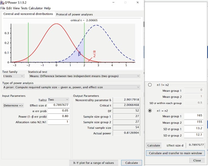
3.5 Example 4: How to Calculate the Sample Size for Comparing Two (Unpaired) Means in Two Populations?
Suppose an investigator is interested in comparing the efficacies of two diet programmes for reducing LDL cholesterol, the following formula can be used for calculating the sample size for each group:
where Z 1−α/2 = 1.96 (For 5% significance level)
Z 1−β = 0.84 (For 80% power)
M1 =165 (mean of LDL cholesterol of Group1)
M2 =155 (mean of LDL cholesterol of Group2)
σ1 = 13.2 (Standard deviation of Group1)
σ2 =12.1 (Standard deviation of Group2)
The formula gives a sample size of 27 for each group.
3.6 Example 5: How to Calculate the Sample Size for Comparing Two Paired Means?
Suppose we are interested in studying the change in behavioural effect following an intervention on the same subjects using pre-test and post-test designs. Here pre- and post-observations are paired. The following formula can be used for estimating the sample size for comparing paired means:
where Z 1−α/2 = 1.96 (For 95% confidence level)
Z 1−β = 1.282 (For 90% power)
d is the effect size = difference of means/ SD
SD = Standard deviation of difference of means = sqrt (σ2 1 + σ2 2 − 2.r. σ1.σ2)
σ1 is the standard deviation(pre)
σ2 is the standard deviation(post)
r is the correlation coefficient between pre- and post-values which is generally not known. In that case, we may assume r = 0.5 for calculating the sample size.
4 Which Are the Free Websites/Software/Apps for Sample Size Calculation?
The following are some of the free websites available on the net for calculation of sample sizes for clinical trials and conducting surveys:
-
1.
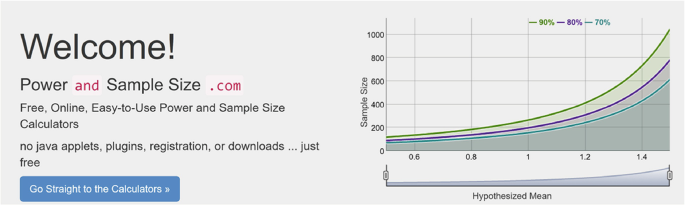
Power and Sample Size: http://powerandsamplesize.com/
This online site hosts a number of sample size calculators for testing means, proportions, odds ratios, and Cox PH. Calculators also have the provision to test the said parameters in superiority, noninferiority, and equivalence mode.
-
2.
G*Power: https://gpower.software.informer.com/3.1/
G*Power is a free downloadable software. It is a powerful tool and includes a large number of programmes for calculating sample sizes for different scenarios. It can do statistical power analyses for many different t tests, F tests, χ 2 tests, z tests, and some exact tests. G*Power can also be used to compute effect sizes and to display graphically the results of power analyses. Below is the snapshot for calculating sample size for testing the difference between two independent means. Here the software first determines the effect size which is transferred to the main window for calculation of the sample size.
-
3.
Statistics and Sample Size App: https://play.google.com/store/apps/details?id=thaithanhtruc.info.stat
This app downloadable from the Google play store is a handy tool to calculate sample size for scientific studies as well as doing basic statistics. It can be used for estimating a proportion in a large and finite population, mean, correlation coefficient, sensitivity, and specificity. Sample size for comparing two proportions (paired and unpaired), two means (paired and unpaired), and multiple means. In addition to this it can be used for case–control, cohort, and survival studies to some extent. Below are the snapshots of the Statistics and Sample Size app for android phones.


-
4.
UCFS-Sample Size Calculators: https://www.sample-size.net/
The online website provides useful calculators for sample size calculation for analytic and descriptive studies for clinical researchers.
-
5.
Sealed envelope: https://www.sealedenvelope.com/power/
The website is suited for determining sample size for superiority, noninferiority, equivalence trials with binary as well as continuous outcomes.
-
6.
OpenEpi: https://www.openepi.com/SampleSize/
The website can be used for calculating sample size for proportion, unmatched case–control, Cohort/RCT, mean difference.
-
7.
R software: https://cran.r-project.org/bin/windows/
R is a free downloadable software and contains useful programs for calculation of sample sizes. It is mainly suited for advanced users who have skills to write and execute the programmes.
5 Which Are Commercial Software Available for Sample Size Calculation?
-
1.
Power and Sample Size (PASS) software: https://www.ncss.com/software/pass/
PASS is a powerful tool for power and sample size calculation. PASS software provides sample size tools for over 965 statistical tests and confidence interval scenarios. It is an extremely user-friendly software tool for power analysis and sample size estimation for testing statistical hypotheses of varying nature in clinical, pharmaceutical, and medical research settings. It includes powerful modules namely—‘group sequential design’ and ‘conditional power’ for power analysis and sample size estimation for carrying out interim analysis of the experimental trials. PASS 2020 is the latest version of the software.
-
2.
Adaptive clinical design software (nQuery): https://www.statsols.com/nquery-adapt/adaptive-clinical-trials
nQuery sample size software includes a whole module dedicated to adaptive clinical trials and is suited for researchers dealing with adaptive clinical trial designs.
-
3.
SAS: https://www.sas.com/en_in/home.html
SAS is a general statistical software package and can be used for calculating sample size and power using its programming language.
6 How Can I Determine Sample Sizes for Diagnostic Test Studies?
Hajian-Tilaki discusses a number of formulae for sample size estimation as well as for testing the sensitivity/specificity, likelihood ratio, and accuracy (AUC) of diagnostic tests. The paper also gives readymade tables of sample sizes for descriptive and diagnostic studies.
7 Summary
Sample size calculation has become a necessity from the ethical and methodological points of view in any research proposal. An underpowered study may fail to detect the treatment effect due to an inadequate sample size, whereas an overpowered study may lead to a waste of resources or may put unnecessarily greater numbers of subjects at risk. Hence, an adequate sample size is required to draw definitive conclusions from a study. Sample size estimation is a large subject and requires in-depth training and expertise, especially when the researcher deals with a complicated study design. A number of software/calculators are available for the calculation of power and sample size. The task becomes easier if the researcher understands the terms associated with these software/calculators/formulae prior to sample size estimation.
Change history
01 July 2022
A correction has been published.
Suggested Reading
Chow SC, Shao J, Wang H, Lokhnygina Y. Sample size calculations in clinical research. 3rd ed. Chapman & Hall/CRC Biostatistics Series; 2019.
Cohen J. A power primer. Psychol Bull. 1992;112:155–9.
Faber J, Fonseca LM. How sample size influences research outcomes. Dental Press J Orthod. 2014;19:27–9.
Author information
Authors and Affiliations
Rights and permissions
Open Access This chapter is licensed under the terms of the Creative Commons Attribution 4.0 International License (http://creativecommons.org/licenses/by/4.0/), which permits use, sharing, adaptation, distribution and reproduction in any medium or format, as long as you give appropriate credit to the original author(s) and the source, provide a link to the Creative Commons license and indicate if changes were made.
The images or other third party material in this chapter are included in the chapter's Creative Commons license, unless indicated otherwise in a credit line to the material. If material is not included in the chapter's Creative Commons license and your intended use is not permitted by statutory regulation or exceeds the permitted use, you will need to obtain permission directly from the copyright holder.
Copyright information
© 2022 The Author(s)
About this chapter

Cite this chapter
Sapra, R.L. (2022). How to Calculate an Adequate Sample Size?. In: How to Practice Academic Medicine and Publish from Developing Countries?. Springer, Singapore. https://doi.org/10.1007/978-981-16-5248-6_9
Download citation
DOI: https://doi.org/10.1007/978-981-16-5248-6_9
Published:
Publisher Name: Springer, Singapore
Print ISBN: 978-981-16-5247-9
Online ISBN: 978-981-16-5248-6
eBook Packages: MedicineMedicine (R0)