Online Causation Monitoring of Signal Temporal Logic

Abstract

Online monitoring is an effective validation approach for hybrid systems, that, at runtime, checks whether the (partial) signals of a system satisfy a specification in, e.g., Signal Temporal Logic (STL). The classic STL monitoring is performed by computing a robustness interval that specifies, at each instant, how far the monitored signals are from violating and satisfying the specification. However, since a robustness interval monotonically shrinks during monitoring, classic online monitors may fail in reporting new violations or in precisely describing the system evolution at the current instant. In this paper, we tackle these issues by considering the causation of violation or satisfaction, instead of directly using the robustness. We first introduce a Boolean causation monitor that decides whether each instant is relevant to the violation or satisfaction of the specification. We then extend this monitor to a quantitative causation monitor that tells how far an instant is from being relevant to the violation or satisfaction. We further show that classic monitors can be derived from our proposed ones. Experimental results show that the two proposed monitors are able to provide more detailed information about system evolution, without requiring a significantly higher monitoring cost.

Z. Zhang is supported by JSPS KAKENHI Grant No. JP23K16865 and No. JP23H03372. J. An, P. Arcaini, and I. Hasuo are supported by ERATO HASUO Metamathematics for Systems Design Project (No. JPMJER1603), JST, Funding Reference number 10.13039/501100009024 ERATO. P. Arcaini is also supported by Engineerable AI Techniques for Practical Applications of High-Quality Machine Learning-based Systems Project (Grant Number JPMJMI20B8), JST-Mirai.

1 Introduction

Safety-critical systems require strong correctness guarantees. Due to the complexity of these systems, offline verification may not be able to guarantee their total correctness, as it is often very difficult to assess all possible system behaviors. To mitigate this issue, runtime verification [4, 29, 36] has been proposed as a complementary technique that analyzes the system execution at runtime. Online monitoring is such an approach that checks whether the system execution (e.g., given in terms of signals) satisfies or violates a system specification specified in a temporal logic [28, 34], e.g., Signal Temporal Logic (STL) [30].

Quantitative online monitoring is based on the STL robust semantics [17, 21] that not only tells whether a signal satisfies or violates a specification $\varphi$ (i.e., the classic Boolean satisfaction relation), but also assigns a value in $\mathbb {R}\cup \{\infty ,-\infty \}$ (i.e., robustness) that indicates how robustly $\varphi$ is satisfied or violated. However, differently from offline assessment of STL formulas, an online monitor needs to reason on partial signals and, so, the assessment of the robustness should be adapted. We consider an established approach [12] employed by classic online monitors (ClaM in the following). It consists in computing, instead of a single robustness value, a robustness interval; at each monitoring step, ClaM identifies an upper bound $\mathrm {[R]}^\textsf{U}$ telling the maximal reachable robustness of any possible suffix signal (i.e., any continuation of the system evolution), and a lower bound $\mathrm {[R]}^\textsf{L}$ telling the minimal reachable robustness. If, at some instant, $\mathrm {[R]}^\textsf{U}$ becomes negative, the specification is violated; if $\mathrm {[R]}^\textsf{L}$ becomes positive, the specification is satisfied. In the other cases, the specification validity is $\texttt{unknown}$.

Fig. 1.

ClaM – Robustness upper and lower bounds of $\Box _{[0,100]}(v < 10)$

Consider a simple example in Fig. 1. It shows the monitoring of the $\texttt{speed}$ of a vehicle (in the upper plot); the specification requires the $\texttt{speed}$ to be always below 10. The lower plot reports how the upper bound $\mathrm {[R]}^\textsf{U}$ and the lower bound $\mathrm {[R]}^\textsf{L}$ of the reachable robustness change over time. We observe that the initial value of $\mathrm {[R]}^\textsf{U}$ is around 8 and gradually decreases.¹ The monitor allows to detect that the specification is violated at time $b = 20$ when the $\texttt{speed}$ becomes higher than 10, and therefore $\mathrm {[R]}^\textsf{U}$ goes below 0. After that, the violation severity progressively gets worse till time $b = 30$, when $\mathrm {[R]}^\textsf{U}$ becomes $-5$. After that point, the monitor does not provide any additional useful information about the system evolution, as $\mathrm {[R]}^\textsf{U}$ remains stuck at $-5$. However, if we observe the signal of the $\texttt{speed}$ after $b = 30$, we notice that (i) the severity of the violation is mitigated, and the “1st violation episode” ends at time $b = 35$; however, the monitor ClaM does not report this type of information; (ii) a “2nd violation episode” occurs in the time interval [40, 45]; the monitor ClaM does not distinguish the new violation.

The reason for the issues reported in the example is that the upper and lower bounds are monotonically decreasing and increasing; this has the that the robustness interval at a given step is “masked” by the history of previous robustness intervals, and, e.g., it is not possible to detect mitigation of the violation severity. Moreover, as an extreme consequence, as soon as the monitor ClaM assesses the violation of the specification (i.e., the upper bound $\mathrm {[R]}^\textsf{U}$ becomes negative), or its satisfaction (i.e., the lower bound $\mathrm {[R]}^\textsf{L}$ becomes positive), the Boolean status of the monitor does not change anymore. Such characteristic directly derives from the STL semantics and it is known as the monotonicity [9,10,11] of classic online monitors. Monotonicity has been recognized as a problem of these monitors in the literature [10, 37, 40], since it does not allow to detect specific types of information that are “masked”. We informally define two types of information masking that can occur because of monotonicity:

• evolution masking: the monitor may not properly report the evolution of the system execution, e.g., mitigation of violation severity may not be detected;

• violation masking: as a special case of evolution masking, the first violation episode during the system execution “masks” the following ones.

The information not reported by ClaM because of information masking, is very useful in several contexts. First of all, in some systems, the first violation of the specification does not mean that the system is not operating anymore, and one may want to continue monitoring and detect all the succeeding violations; this is the case, e.g., of the monitoring approach reported by Selyunin et al. [37] in which all the violations of the SENT protocol must be detected. Moreover, having a precise description of the system evolution is important for the usefulness of the monitoring; for example, the monitoring of the $\texttt{speed}$ in Fig. 1 could be used in a vehicle for checking the speed and notifying the driver whenever the speed is approaching the critical limit; if the monitor is not able to precisely capture the severity of violation, it cannot be used for this type of application.

Some works [10, 37, 40] try to mitigate the monotonicity issues, by “resetting” the monitor at specific points. A recent approach has been proposed by Zhang et al. [40] (called ResM in the following) that is able to identify each “violation episode” (i.e., it solves the problem of violation masking), but does not solve the evolution masking problem. For the example in Fig. 1, ResM is able to detect the two violation episodes in intervals [20, 35] and [40, 45], but it is not able to report that the speed decreases after $b = 10$ (in a non-violating situation), and that the severity of the violation is mitigated after $b = 30$.

Contribution. In this paper, in order to provide more information about the evolution of the monitored system, we propose to monitor the causation of violation or satisfaction, instead of considering the robustness directly. To do this, we rely on the notion of epoch [5]. At each instant, the violation (satisfaction) epoch identifies the time instants at which the evaluation of the atomic propositions of the specification $\varphi$ causes the violation (satisfaction) of $\varphi$.

Based on the notion of epoch, we define a Boolean causation monitor (called BCauM) that, at runtime, not only assesses the specification violation/satisfaction, but also tells whether each instant is relevant to it. Namely, BCauM marks each current instant $b$ as (i) a violation causation instant, if $b$ is added to the violation epoch; (ii) a satisfaction causation instant, if $b$ is added to the satisfaction epoch; (iii) an irrelevant instant, if $b$ is not added to any epoch. We show that BCauM is able to detect all the violation episodes (so solving the violation masking issue), as violation causation instants can be followed by irrelevant instants. Moreover, we show that the information provided by the classic Boolean online monitor can be derived from that of the Boolean causation monitor BCauM.

However, BCauM just tells us whether the current instant is a (violation or satisfaction) causation instant or not, but does not report how far the instant is from being a causation instant. To this aim, we introduce the notion of causation distance, as a quantitative measure characterizing the spatial distance of the signal value at b from turning b into a causation instant. Then, we propose the quantitative causation monitor (QCauM) that, at each instant, returns its causation distance. We show that using QCauM, besides solving the violation masking problem, we also solve the evolution masking problem. Moreover, we show that we can derive from QCauM both the classic quantitative monitor ClaM, and the Boolean causation monitor BCauM.

Experimental results show that the proposed monitors, not only provide more information, but they do it in an efficient way, not requiring a significant additional monitoring time w.r.t. the existing monitors.

Outline. Section 2 reports necessary background. We introduce BCauM in Sect. 3, and QCauM in Sect. 4. Experimental assessment of the two proposed monitors is reported in Sect. 5. Finally, Sect. 6 discusses some related work, and Sect. 7 concludes the paper.

2 Preliminaries

In this section, we review the fundamentals of signal temporal logic (STL) in Sect. 2.1, and then introduce the existing classic online monitoring approach in Sect. 2.2.

2.1 Signal Temporal Logic

Let $T\in \mathbb {R}_{+}$ be a positive real, and $d \in \mathbb {N}_{+}$ be a positive integer. A $d$-dimensional signal is a function $\textbf{v} :[0,T]\rightarrow \mathbb {R}^ d$, where T is called the time horizon of $\textbf{v}$. Given an arbitrary time instant $t\in [0, T]$, $\textbf{v} (t)$ is a $d$-dimensional real vector; each dimension concerns a signal variable that has a certain physical meaning, e.g., $\texttt{speed}$, $\texttt{RPM}$, $\texttt{acceleration}$, etc. In this paper, we fix a set $\textbf{Var}$ of variables and assume that a signal $\textbf{v}$ is spatially bounded, i.e., for all $t\in [0, T]$, $\textbf{v} (t)\in \varOmega$, where $\varOmega$ is a $d$-dimensional hyper-rectangle.

Signal temporal logic (STL) is a widely-adopted specification language, used to describe the expected behavior of systems. In Definition 1 and Definition 2, we respectively review the syntax and the robust semantics of STL [17, 21, 30].

Definition 1

(STL syntax). In STL, the atomic propositions $\alpha$ and the formulas $\varphi$ are defined as follows:

$$\begin{aligned}&\alpha \,{:}{:}\equiv \, f(w_1, \dots , w_K) > 0 \qquad&\varphi \,{:}{:}\equiv \, \alpha \mid \bot \mid \lnot \varphi \mid \varphi \wedge \varphi \mid \Box _{I}\varphi \mid \Diamond _{I}\varphi \mid \varphi \mathbin {\mathcal {U}_{I}} \varphi \end{aligned}$$

Here f is a K-ary function $f:\mathbb {R}^K \rightarrow \mathbb {R}$, $w_1, \dots , w_K \in \textbf{Var}$, and I is a closed interval over $\mathbb {R}_{\ge 0}$, i.e., $I=[l,u]$, where $l,u \in \mathbb {R}$ and $l\le u$. In the case that $l = u$, we can use l to stand for I. $\Box , \Diamond$ and $\mathcal {U}$ are temporal operators, which are known as always, eventually and until, respectively. The always operator $\Box$ and eventually operator $\Diamond$ are two special cases of the until operator $\mathcal {U}$, where $\Diamond _{I}\varphi \equiv \top \mathbin {\mathcal {U}_{I}}\varphi$ and $\Box _{I}\varphi \equiv \lnot \Diamond _{I}\lnot \varphi$. Other common connectives such as $\vee , \rightarrow$ are introduced as syntactic sugar: $\varphi _1\vee \varphi _2\equiv \lnot (\lnot \varphi _1\wedge \lnot \varphi _2)$, $\varphi _1\rightarrow \varphi _2 \equiv \lnot \varphi _1 \vee \varphi _2$.

Definition 2

(STL robust semantics). Let $\textbf{v}$ be a signal, $\varphi$ be an STL formula and $\tau \in \mathbb {R}_{+}$ be an instant. The robustness $\textrm{R}(\textbf{v}, \varphi , \tau ) \in \mathbb {R}\cup \{\infty ,-\infty \}$ of $\textbf{v}$ w.r.t. $\varphi$ at $\tau$ is defined by induction on the construction of formulas, as follows.

$$\begin{aligned}&\textrm{R}(\textbf{v}, \alpha , \tau ) \;:=\; f(\textbf{v} (\tau )) \qquad \textrm{R}(\textbf{v}, \bot , \tau ) \;:=\; -\infty \qquad \textrm{R}(\textbf{v}, \lnot \varphi , \tau ) \;:=\; -\textrm{R}(\textbf{v}, \varphi , \tau ) \\&\textrm{R}(\textbf{v}, \varphi _1\wedge \varphi _2, \tau ) \;:=\; \min \left( \textrm{R}(\textbf{v}, \varphi _1, \tau ), \textrm{R}(\textbf{v}, \varphi _2, \tau )\right) \\&\textrm{R}(\textbf{v}, \Box _{I}\varphi , \tau ) \;:=\; \inf _{t\in \tau + I}{\textrm{R}(\textbf{v}, \varphi , t)} \qquad \textrm{R}(\textbf{v}, \Diamond _{I}\varphi , \tau ) \;:=\; \sup _{t\in \tau + I}{\textrm{R}(\textbf{v}, \varphi , t)} \\&\textrm{R}(\textbf{v}, \varphi _1 \mathbin {\mathcal {U}_{I}} \varphi _2, \tau ) \;:=\; \sup _{t \in \tau + I} \min \left( \textrm{R}(\textbf{v}, \varphi _2, t), \inf _{t' \in [\tau , t)} \textrm{R}(\textbf{v}, \varphi _1, t') \right) \end{aligned}$$

Here, $\tau + I$ denotes the interval $[l+\tau , u+\tau ]$.

The original STL semantics is Boolean, which represents whether a signal $\textbf{v}$ satisfies $\varphi$ at an instant $\tau$, i.e., whether $(\textbf{v}, \tau ) \models \varphi$. The robust semantics in Definition 2 is a quantitative extension that refines the original Boolean STL semantics, in the sense that, $\textrm{R}(\textbf{v}, \varphi , \tau ) > 0$ implies $(\textbf{v}, \tau )\models \varphi$, and $\textrm{R}(\textbf{v}, \varphi , \tau ) < 0$ implies $(\textbf{v}, \tau )\not \models \varphi$. More details can be found in [21, Proposition 16].

2.2 Classic Online Monitoring of STL

STL robust semantics in Definition 2 provides an offline monitoring approach for complete signals. Online monitoring, instead, targets a growing partial signal at runtime. Besides the verdicts $\top$ and $\bot$, an online monitor can also report the verdict $\texttt{unknown}$ (denoted as $\mathord {?}$), which represents a status when the satisfaction of the signal to $\varphi$ is not decided yet. In the following, we formally define partial signals and introduce online monitors for STL.

Let T be the time horizon of a signal $\textbf{v}$, and let $[a, b]\subseteq [0, T]$ be a sub-interval in the time domain [0, T]. A partial signal $\textbf{v}_{a:b}$ is a function which is only defined in the interval [a, b]; in the remaining domain $[0,T]\setminus [a, b]$, we denote that $\textbf{v}_{a:b} = \epsilon$, where $\epsilon$ stands for a value that is not defined.

Specifically, if $a = 0$ and $b\in (a, T]$, a partial signal $\textbf{v}_{a:b}$ is called a prefix (partial) signal; dually, if $b = T$ and $a\in [0, b)$, a partial signal $\textbf{v}_{a:b}$ is called a suffix (partial) signal. Given a prefix signal $\textbf{v}_{0:b}$, a completion $\textbf{v}_{0:b} \cdot \textbf{v}_{b:T}$ of $\textbf{v}_{0:b}$ is defined as the concatenation of $\textbf{v}_{0:b}$ with a suffix signal $\textbf{v}_{b:T}$.

Definition 3

(Classic Boolean STL online monitor). Let $\textbf{v}_{0:b}$ be a prefix signal, and $\varphi$ be an STL formula. An online monitor $\textrm{M}(\textbf{v}_{0:b}, \varphi , \tau )$ returns a verdict in $\{\top , \bot , \mathord {?} \}$ (namely, $\texttt{true}$, $\texttt{false}$, and $\texttt{unknown}$), as follows:

$$\begin{aligned} \textrm{M}(\textbf{v}_{0:b}, \varphi , \tau ) \;:=\; {\left\{ \begin{array}{ll} \top &{} \text {if } \forall \textbf{v}_{b:T}.\, \textrm{R}(\textbf{v}_{0:b} \cdot \textbf{v}_{b:T}, \varphi , \tau ) > 0 \\ \bot &{} \text {if } \forall \textbf{v}_{b:T}.\, \textrm{R}(\textbf{v}_{0:b} \cdot \textbf{v}_{b:T}, \varphi , \tau ) < 0\\ \mathord {?} &{} \text {otherwise} \end{array}\right. } \end{aligned}$$

Namely, the verdicts of $\textrm{M}(\textbf{v}_{0:b}, \varphi , \tau )$ are interpreted as follows:

• if any possible completion $\textbf{v}_{0:b} \cdot \textbf{v}_{b:T}$ of $\textbf{v}_{0:b}$ satisfies $\varphi$, then $\textbf{v}_{0:b}$ satisfies $\varphi$;

• if any possible completion $\textbf{v}_{0:b} \cdot \textbf{v}_{b:T}$ of $\textbf{v}_{0:b}$ violates $\varphi$, then $\textbf{v}_{0:b}$ violates $\varphi$;

• otherwise (i.e., there is a completion $\textbf{v}_{0:b} \cdot \textbf{v}_{b:T}$ that satisfies $\varphi$, and there is a completion $\textbf{v}_{0:b} \cdot \textbf{v}_{b:T}$ that violates $\varphi$), then $\textrm{M}(\textbf{v}_{0:b}, \varphi , \tau )$ reports $\texttt{unknown}$.

Note that, by Definition 3 only, we cannot synthesize a feasible online monitor, because the possible completions for $\textbf{v}_{0:b}$ are infinitely many. A constructive online monitor is introduced in [12], which implements the functionality of Definition 3 by computing the reachable robustness of $\textbf{v}_{0:b}$. We review this monitor in Definition 4.

Definition 4

(Classic Quantitative STL online monitor (ClaM)). Let $\textbf{v}_{0:b}$ be a prefix signal, and let $\varphi$ be an STL formula. We denote by $\texttt{R}^{\alpha }_{\textrm{max}}$ and $\texttt{R}^{\alpha }_{\textrm{min}}$ the possible maximum and minimum bounds of the robustness $\textrm{R}(\textbf{v}, \alpha , \tau )$². Then, an online monitor $\mathrm {[R]}(\textbf{v}_{0:b}, \varphi , \tau )$, which returns a sub-interval of $[\texttt{R}^{\alpha }_{\textrm{min}}, \texttt{R}^{\alpha }_{\textrm{max}}]$ at the instant b, is defined as follows, by induction on the construction of formulas.

$$\begin{aligned}&\mathrm {[R]}(\textbf{v}_{0:b}, \alpha , \tau ) \;:=\; {\left\{ \begin{array}{ll} \big [f\left( \textbf{v}_{0:b} (\tau )\right) , f\left( \textbf{v}_{0:b} (\tau )\right) \big ] &{} \text {if } \tau \in [0, b]\\ \big [\texttt{R}^{\alpha }_{\textrm{min}}, \texttt{R}^{\alpha }_{\textrm{max}}\big ]&{} \text {otherwise} \end{array}\right. }\\&\mathrm {[R]}(\textbf{v}_{0:b}, \lnot \varphi , \tau ) \;:=\; - \mathrm {[R]}(\textbf{v}_{0:b}, \varphi , \tau ) \\&\mathrm {[R]}(\textbf{v}_{0:b}, \varphi _1\wedge \varphi _2, \tau ) \;:=\; \min \Big (\mathrm {[R]}(\textbf{v}_{0:b}, \varphi _1, \tau ), \mathrm {[R]}(\textbf{v}_{0:b}, \varphi _2, \tau )\Big ) \\&\mathrm {[R]}(\textbf{v}_{0:b}, \Box _I\varphi , \tau ) \;:=\; \inf _{t\in \tau +I}\Big (\mathrm {[R]}(\textbf{v}_{0:b}, \varphi , t)\Big ) \\&\mathrm {[R]}(\textbf{v}_{0:b}, \varphi _1\mathbin {\mathcal {U}_{I}}\varphi _2, \tau ) \;:=\; \sup _{t\in \tau +I}\min \Big (\mathrm {[R]}(\textbf{v}_{0:b}, \varphi _2, t), \inf _{t'\in [\tau , t)}\mathrm {[R]}(\textbf{v}_{0:b}, \varphi _1, t')\Big ) \end{aligned}$$

Here, f is defined as in Definition 1, and the arithmetic rules over intervals $I=[l, u]$ are defined as follows: $-I:=[-u, -l] \text { and } \min (I_1,I_2) :=[\min (l_1, l_2), \min (u_1, u_2)]$.

We denote by $\mathrm {[R]}^\textsf{U}(\textbf{v}_{0:b}, \varphi , \tau )$ and $\mathrm {[R]}^\textsf{L}(\textbf{v}_{0:b}, \varphi , \tau )$ the upper bound and the lower bound of $\mathrm {[R]}(\textbf{v}_{0:b}, \varphi , \tau )$ respectively. Intuitively, the two bounds together form the reachable robustness interval of the completion $\textbf{v}_{0:b} \cdot \textbf{v}_{b:T}$, under any possible suffix signal $\textbf{v}_{b:T}$. For instance, in Fig. 2, the upper bound $\mathrm {[R]}^\textsf{U}$ at $b= 20$ is 0, which indicates that the robustness of the completion of the signal $\texttt{speed}$, under any suffix, can never be larger than 0.

The quantitative online monitor ClaM in Definition 4 refines the Boolean one in Definition 3, and the Boolean monitor can be derived from ClaM as follows:

• if $\mathrm {[R]}^\textsf{L}(\textbf{v}_{0:b}, \varphi , \tau ) > 0$, it implies that $\textrm{M}(\textbf{v}_{0:b}, \varphi , \tau ) = \top$;

• if $\mathrm {[R]}^\textsf{U}(\textbf{v}_{0:b}, \varphi , \tau ) < 0$, it implies that $\textrm{M}(\textbf{v}_{0:b}, \varphi , \tau ) = \bot$;

• otherwise, if $\mathrm {[R]}^\textsf{L}(\textbf{v}_{0:b}, \varphi , \tau ) < 0$ and $\mathrm {[R]}^\textsf{U}(\textbf{v}_{0:b}, \varphi , \tau ) > 0$, $\textrm{M}(\textbf{v}_{0:b}, \varphi , \tau ) = \mathord {?}$.

The classic online monitors are monotonic by definition. In the Boolean monitor (Definition 3), with the growth of $\textbf{v}_{0:b}$, $\textrm{M}(\textbf{v}_{0:b}, \varphi , \tau )$ can only turn from $\mathord {?}$ to $\{\bot , \top \}$, but never the other way around. In the quantitative one (Definition 4), as shown in Lemma 1, $\mathrm {[R]}^\textsf{U}(\textbf{v}_{0:b}, \varphi , \tau )$ and $\mathrm {[R]}^\textsf{L}(\textbf{v}_{0:b}, \varphi , \tau )$ are both monotonic, the former one decreasingly, the latter one increasingly. An example can be observed in Fig. 2.

Lemma 1

(Monotonicity of STL online monitor). Let $\mathrm {[R]}(\textbf{v}_{0:b}, \varphi , \tau )$ be the quantitative online monitor for a partial signal $\textbf{v}_{0:b}$ and an STL formula $\varphi$. With the growth of the partial signal $\textbf{v}_{0:b}$, the upper bound $\mathrm {[R]}^\textsf{U}(\textbf{v}_{0:b}, \varphi , \tau )$ monotonically decreases, and the lower bound $\mathrm {[R]}^\textsf{L}(\textbf{v}_{0:b}, \varphi , \tau )$ monotonically increases, i.e., for two time instants $b_1, b_2 \in [0, T]$, if $b_1 < b_2$, we have (i) $\mathrm {[R]}^\textsf{U}(\textbf{v}_{0:b_1}, \varphi , \tau ) \ge \mathrm {[R]}^\textsf{U}(\textbf{v}_{0:b_2}, \varphi , \tau )$, and (ii) $\mathrm {[R]}^\textsf{L}(\textbf{v}_{0:b_1}, \varphi , \tau ) \le \mathrm {[R]}^\textsf{L}(\textbf{v}_{0:b_2}, \varphi , \tau )$.

Proof

This can be proved by induction on the structures of STL formulas. The detailed proof can be found in the full version [38].    $\square$

3 Boolean Causation Online Monitor

As explained in Sect. 1, monotonicity of classic online monitors causes different types of information masking, which prevents some information from being delivered. In this section, we introduce a novel Boolean causation (online) monitor BCauM, that solves the violation masking issue (see Sect. 1). BCauM is defined based on online signal diagnostics [5, 40], which reports the cause of violation or satisfaction of the specification at the atomic proposition level.

Definition 5

(Online signal diagnostics). Let $\textbf{v}_{0:b}$ be a partial signal and $\varphi$ be an STL specification. At an instant b, online signal diagnostics returns a violation epoch $\textrm{E}^{\ominus }(\textbf{v}_{0:b}, \varphi , \tau )$, under the condition $\mathrm {[R]}^\textsf{U}(\textbf{v}_{0:b}, \varphi , \tau ) < 0$, as follows:

and a satisfaction epoch $\textrm{E}^{\oplus }(\textbf{v}_{0:b}, \varphi , \tau )$, under the condition $\mathrm {[R]}^\textsf{L}(\textbf{v}_{0:b}, \varphi , \tau )>0$, as follows:

If the conditions are not satisfied, $\textrm{E}^{\ominus }(\textbf{v}_{0:b}, \varphi , \tau )$ and $\textrm{E}^{\oplus }(\textbf{v}_{0:b}, \varphi , \tau )$ are both $\emptyset$. Note that the definition is recursive, thus the conditions should also be checked for computing the violation and satisfaction epochs of the sub-formulas of $\varphi$.

Computation for other operators can be inferred by the presented ones and the STL syntax (Definition 1).

Intuitively, when a partial signal $\textbf{v}_{0:b}$ violates a specification $\varphi$, a violation epoch starts collecting the evaluations (identified by pairs of atomic propositions and instants) of the signal at the atomic proposition level, that cause the violation of the whole formula $\varphi$ (which also applies to the satisfaction cases in a dual manner). This is done inductively, based on the semantics of different operators:

• in the case of an atomic proposition $\alpha$, if $\alpha$ is violated at $\tau$, it collects $\langle \alpha , \tau \rangle$;

• in the case of a negation $\lnot \varphi$, it collects the satisfaction epoch of $\varphi$;

• in the case of a conjunction $\varphi _1\wedge \varphi _2$, it collects the union of the violation epochs of the sub-formulas violated by the partial signal;

• in the case of an always operator $\Box _I\varphi$, it collects the epochs of the sub-formula $\varphi$ at all the instants t where $\varphi$ is evaluated as being violated.

• in the case of an until operator $\varphi _1 \mathbin {\mathcal {U}_{I}} \varphi _2$, it collects the epochs of the sub-formula $\varphi _2$ at all the instants t and the epochs of $\varphi _1$ at the instants $t'\in [\tau ,t)$, in the case where the clause “$\varphi _1$ until $\varphi _2$” is violated at t.

Fig. 2.

Classic monitor (ClaM) result for the STL specification: $\Box _{[0,100]}(v>10 \rightarrow \Diamond _{[0,5]}(a<0))$

Fig. 3.

The violation epochs (the red parts) respectively when $b= 30$ and $b=35$

Fig. 4.

Boolean causation monitor (BCauM) result

Example 1

The example in Fig. 2 illustrates how an epoch is collected. The specification requires that whenever the $\texttt{speed}$ is higher than 10, the car should decelerate within 5 time units. As shown by the classic monitor, the specification is violated at $b = 25$, since v becomes higher than 10 at 20 but a remains positive during [20, 25]. Note that the specification can be rewritten as $\varphi \equiv \Box _{[0,100]}(\lnot (v>10)\vee \Diamond _{[0,5]}(a<0))$. For convenience, we name the sub-formulas of $\varphi$ as follows:

$$\begin{aligned} \begin{array}{c} \varphi ' \equiv \lnot (v>10)\vee \Diamond _{[0,5]}(a<0) \qquad \varphi _1\equiv \lnot (v>10) \qquad \varphi _2\equiv \Diamond _{[0,5]}(a<0) \\ \alpha _1 \equiv v >10 \qquad \alpha _2 \equiv a< 0 \end{array} \end{aligned}$$

Figure 3 shows the violation epochs at two instants 30 and 35. First, at $b = 30$,

$$\begin{aligned} \textrm{E}^{\ominus }(\textbf{v}_{0:30}, \varphi , 0)&= \big (\textstyle \bigcup _{t\in [20, 25]}\textrm{E}^{\oplus }(\textbf{v}_{0:30}, \alpha _1, t)\big ) \cup \big (\textstyle \bigcup _{t\in [20,30]}\textrm{E}^{\ominus }(\textbf{v}_{0:30}, \alpha _2, t)\big ) \\&= \langle \alpha _1, [20, 25]\rangle \cup \langle \alpha _2, [20, 30]\rangle \end{aligned}$$

Similarly, the violation epoch $\textrm{E}^{\ominus }(\textbf{v}_{0:35}, \varphi , 0)$ at $b=35$ is the same as that at $b = 30$. Intuitively, the epoch at $b = 30$ shows the cause of the violation of $\textbf{v}_{0:30}$; then since signal $a<0$ in [30, 35], this segment is not considered as the cause of the violation, so the epoch remains the same at $b = 35$. $\lhd$

Definition 6

(Boolean causation monitor (BCauM)). Let $\textbf{v}_{0:b}$ be a partial signal and $\varphi$ be an STL specification. We denote by $\mathcal {A}$ the set of atomic propositions of $\varphi$. At each instant b, a Boolean causation (online) monitor BCauM returns a verdict in $\{\ominus , \oplus , \oslash \}$ (called violation causation, satisfaction causation and irrelevant), which is defined as follows,

$$\begin{aligned} \mathscr {M}(\textbf{v}_{0:b}, \varphi , \tau ) \;:=\; {\left\{ \begin{array}{ll} \ominus &{} \text {if } \exists \alpha \in \mathcal {A}.\;\langle \alpha , b\rangle \in \textrm{E}^{\ominus }(\textbf{v}_{0:b}, \varphi , \tau ) \\ \oplus &{} \text {if }\exists \alpha \in \mathcal {A}.\;\langle \alpha , b\rangle \in \textrm{E}^{\oplus }(\textbf{v}_{0:b}, \varphi , \tau ) \\ \oslash &{} \text {otherwise} \end{array}\right. } \end{aligned}$$

An instant b is called a violation/satisfaction causation instant if $\mathscr {M}(\textbf{v}_{0:b}, \varphi , \tau )$ returns $\ominus$/$\oplus$, or an irrelevant instant if $\mathscr {M}(\textbf{v}_{0:b}, \varphi , \tau )$ returns $\oslash$.

Intuitively, if the current instant b (with the related $\alpha$) is included in the epoch (thus the signal value at b is relevant to the violation/satisfaction of $\varphi$), BCauM will report a violation/satisfaction causation ($\ominus$/$\oplus$); otherwise, it will report irrelevant ($\oslash$). Notably BCauM is non-monotonic, in that even if it reports $\ominus$ or $\oplus$ at some instant b, it may still report $\oslash$ after b. This feature allows BCauM to bring more information, e.g., it can detect the end of a violation episode and the start of a new one (i.e., it solves the violation masking issue in Sect. 1); see Example 2.

Example 2

Based on the signal diagnostics in Fig. 3, the Boolean causation monitor BCauM reports the result shown as in Fig. 4.

Compared to the classic Boolean monitor in Fig. 2, BCauM brings more information, in the sense that it detects the end of the violation episode at $b = 30$, by going from $\ominus$ to $\oslash$, when the signal a becomes negative. $\lhd$

Theorem 1 states the relation of BCauM with the classic Boolean online monitor.

Theorem 1

The Boolean causation monitor BCauM in Definition 6 refines the classic Boolean online monitor in Definition 3, in the following sense:

• $\textrm{M}(\textbf{v}_{0:b}, \varphi , \tau ) = \bot \quad \textit{iff.}\quad \bigvee _{t\in [0,b]}\left( \mathscr {M}(\textbf{v}_{0:t}, \varphi , \tau ) = \ominus \right)$

• $\textrm{M}(\textbf{v}_{0:b}, \varphi , \tau ) = \top \quad \textit{iff.}\quad \bigvee _{t\in [0,b]}\left( \mathscr {M}(\textbf{v}_{0:t}, \varphi , \tau ) = \oplus \right)$

• $\textrm{M}(\textbf{v}_{0:b}, \varphi , \tau ) = \,\mathord {?} \, \quad \textit{iff.}\quad \bigwedge _{t\in [0,b]}\left( \mathscr {M}(\textbf{v}_{0:t}, \varphi , \tau ) = \oslash \right)$

Proof

The proof is based on Definitions 5 and 6, Lemma 1 about the monotonicity of classic STL online monitors, and two extra lemmas in the full version [38].

   $\square$

4 Quantitative Causation Online Monitor

Although BCauM in Sect. 3 is able to solve the violation masking issue, it still does not provide enough information about the evolution of the system signals, i.e., it does not solve the evolution masking issue introduced in Sect. 1. To tackle this issue, we propose a quantitative (online) causation monitor QCauM in Definition 7, which is a quantitative extension of BCauM. Given a partial signal $\textbf{v}_{0:b}$, QCauM reports a violation causation distance ${[\mathscr {R}]}^\ominus \left( \textbf{v}_{0:b}, \varphi , \tau \right)$ and a satisfaction causation distance ${[\mathscr {R}]}^\oplus \left( \textbf{v}_{0:b}, \varphi , \tau \right)$, which, respectively, indicate how far the signal value at the current instant $b$ is from turning $b$ into a violation causation instant and from turning $b$ into a satisfaction causation instant.

Definition 7

(Quantitative causation monitor (QCauM)). Let $\textbf{v}_{0:b}$ be a partial signal, and $\varphi$ be an STL specification. At instant b, the quantitative causation monitor QCauM returns a violation causation distance ${[\mathscr {R}]}^\ominus \left( \textbf{v}_{0:b}, \varphi , \tau \right)$, as follows:

$$\begin{aligned}&{[\mathscr {R}]}^\ominus \left( \textbf{v}_{0:b}, \alpha , \tau \right) \;:=\; {\left\{ \begin{array}{ll} f(\textbf{v}_{0:b} (\tau )) &{} \text {if } b = \tau \\ \texttt{R}^{\alpha }_{\textrm{max}}&{} \text {otherwise} \end{array}\right. }\\&{[\mathscr {R}]}^\ominus \left( \textbf{v}_{0:b}, \lnot \varphi , \tau \right) \;:=\; -{[\mathscr {R}]}^\oplus \left( \textbf{v}_{0:b}, \varphi , \tau \right) \\&{[\mathscr {R}]}^\ominus \left( \textbf{v}_{0:b}, \varphi _1\wedge \varphi _2, \tau \right) \;:=\; \min \left( {[\mathscr {R}]}^\ominus \left( \textbf{v}_{0:b}, \varphi _1, \tau \right) , {[\mathscr {R}]}^\ominus \left( \textbf{v}_{0:b}, \varphi _2, \tau \right) \right) \\&{[\mathscr {R}]}^\ominus \left( \textbf{v}_{0:b}, \varphi _1\vee \varphi _2, \tau \right) \;:=\; \min \left( \begin{array}{l} \max \left( {[\mathscr {R}]}^\ominus \left( \textbf{v}_{0:b}, \varphi _1, \tau \right) , \mathrm {[R]}^\textsf{U}(\textbf{v}_{0:b}, \varphi _2, \tau ) \right) , \\ \max \left( \mathrm {[R]}^\textsf{U}(\textbf{v}_{0:b}, \varphi _1, \tau ), {[\mathscr {R}]}^\ominus \left( \textbf{v}_{0:b}, \varphi _2, \tau \right) \right) \end{array} \right) \end{aligned}$$

$$\begin{aligned}&{[\mathscr {R}]}^\ominus \left( \textbf{v}_{0:b}, \Box _I\varphi , \tau \right) \;:=\; \inf _{t\in \tau +I}\left( {[\mathscr {R}]}^\ominus \left( \textbf{v}_{0:b}, \varphi , t\right) \right) \\&{[\mathscr {R}]}^\ominus \left( \textbf{v}_{0:b}, \Diamond _I\varphi , \tau \right) \;:=\; \inf _{t\in \tau +I}\left( \max \left( {[\mathscr {R}]}^\ominus \left( \textbf{v}_{0:b}, \varphi , t\right) , \mathrm {[R]}^\textsf{U}(\textbf{v}_{0:b}, \Diamond _I\varphi , \tau ) \right) \right) \\&{[\mathscr {R}]}^\ominus \left( \textbf{v}_{0:b}, \varphi _1\mathbin {\mathcal {U}_{I}}\varphi _2, \tau \right) \;:=\; \inf _{t\in \tau +I}\left( \max \left( \begin{array}{l} \min \left( \begin{array}{l} \displaystyle \inf _{t'\in [\tau ,t)}{[\mathscr {R}]}^\ominus \left( \textbf{v}_{0:b}, \varphi _1, t'\right) \\ {[\mathscr {R}]}^\ominus \left( \textbf{v}_{0:b}, \varphi _2, t\right) \end{array} \right) \\ \mathrm {[R]}^\textsf{U}(\textbf{v}_{0:b}, \varphi _1\mathbin {\mathcal {U}_{I}}\varphi _2, \tau ) \end{array} \right) \right) \end{aligned}$$

and a satisfaction causation distance ${[\mathscr {R}]}^\oplus \left( \textbf{v}_{0:b}, \varphi , \tau \right)$, as follows:

$$\begin{aligned}&{[\mathscr {R}]}^\oplus \left( \textbf{v}_{0:b}, \alpha , \tau \right) \;:=\; {\left\{ \begin{array}{ll} f(\textbf{v}_{0:b} (\tau )) &{} \text {if } b = \tau \\ \texttt{R}^{\alpha }_{\textrm{min}}&{} \text {otherwise} \end{array}\right. }\\&{[\mathscr {R}]}^\oplus \left( \textbf{v}_{0:b}, \lnot \varphi , \tau \right) \;:=\; - {[\mathscr {R}]}^\ominus \left( \textbf{v}_{0:b}, \varphi , \tau \right) \\&{[\mathscr {R}]}^\oplus \left( \textbf{v}_{0:b}, \varphi _1\wedge \varphi _2, \tau \right) \;:=\; \max \left( \begin{array}{l} \min \left( {[\mathscr {R}]}^\oplus \left( \textbf{v}_{0:b}, \varphi _1, \tau \right) , \mathrm {[R]}^\textsf{L}(\textbf{v}_{0:b}, \varphi _2, \tau ) \right) , \\ \min \left( \mathrm {[R]}^\textsf{L}(\textbf{v}_{0:b}, \varphi _1, \tau ), {[\mathscr {R}]}^\oplus \left( \textbf{v}_{0:b}, \varphi _2, \tau \right) \right) \end{array} \right) \\&{[\mathscr {R}]}^\oplus \left( \textbf{v}_{0:b}, \varphi _1\vee \varphi _2, \tau \right) \;:=\; \max \left( {[\mathscr {R}]}^\oplus \left( \textbf{v}_{0:b}, \varphi _1, \tau \right) , {[\mathscr {R}]}^\oplus \left( \textbf{v}_{0:b}, \varphi _2, \tau \right) \right) \\&{[\mathscr {R}]}^\oplus \left( \textbf{v}_{0:b}, \Box _I\varphi , \tau \right) \;:=\; \sup _{t\in \tau +I}\left( \min \left( {[\mathscr {R}]}^\oplus \left( \textbf{v}_{0:b}, \varphi , t\right) , \mathrm {[R]}^\textsf{L}(\textbf{v}_{0:b}, \Box _I\varphi , \tau ) \right) \right) \\&{[\mathscr {R}]}^\oplus \left( \textbf{v}_{0:b}, \Diamond _I\varphi , \tau \right) \;:=\; \sup _{t\in \tau +I}\left( {[\mathscr {R}]}^\oplus \left( \textbf{v}_{0:b}, \varphi , t\right) \right) \\&{[\mathscr {R}]}^\oplus \left( \textbf{v}_{0:b}, \varphi _1\mathbin {\mathcal {U}_{I}}\varphi _2, \tau \right) :=\sup _{t\in \tau +I}\left( \max \left( \begin{array}{l} \min \left( \begin{array}{l} \displaystyle \sup _{t'\in [\tau , t)}{[\mathscr {R}]}^\oplus \left( \textbf{v}_{0:b}, \varphi _1, t'\right) \\ \displaystyle \inf _{t'\in [\tau , t)}\mathrm {[R]}^\textsf{L}(\textbf{v}_{0:b}, \varphi _1, t')\\ \mathrm {[R]}^\textsf{L}(\textbf{v}_{0:b}, \varphi _2, t) \end{array} \right) \\ \min \left( \begin{array}{l} \displaystyle \inf _{t'\in [\tau , t)}\mathrm {[R]}^\textsf{L}(\textbf{v}_{0:b}, \varphi _1, t') \\ {[\mathscr {R}]}^\oplus \left( \textbf{v}_{0:b}, \varphi _2, t\right) \end{array} \right) \end{array} \right) \right) \end{aligned}$$

Intuitively, a violation causation distance ${[\mathscr {R}]}^\ominus \left( \textbf{v}_{0:b}, \varphi , \tau \right)$ is the spatial distance of the signal value $\textbf{v}_{0:b} (b)$, at the current instant b, from turning b into a violation causation instant such that b is relevant to the violation of $\varphi$ (also applied to the satisfaction case dually). It is computed inductively on the structure of $\varphi$:

• Case atomic propositions $\alpha$: if $b = \tau$ (i.e., at which instant $\alpha$ should be evaluated), then the distance of b from being a violation causation instant is $f(\textbf{v}_{0:b} (b))$; otherwise, if $b\ne \tau$, despite the value of $f(\textbf{v}_{0:b} (b))$, b can never be a violation causation instant, according to Definition 5, because only $f(\textbf{v}_{0:b} (\tau ))$ is relevant to the violation of $\alpha$. Hence, the distance will be $\texttt{R}^{\alpha }_{\textrm{max}}$;

• Case $\lnot \varphi$: b is a violation causation instant for $\lnot \varphi$ if b is a satisfaction causation instant for $\varphi$, so ${[\mathscr {R}]}^\ominus \left( \textbf{v}_{0:b}, \lnot \varphi , \tau \right)$ depends on ${[\mathscr {R}]}^\oplus \left( \textbf{v}_{0:b}, \varphi , \tau \right)$;

• Case $\varphi _1\wedge \varphi _2$: b is a violation causation instant for $\varphi _1\wedge \varphi _2$ if b is a violation causation instant for either $\varphi _1$ or $\varphi _2$, so ${[\mathscr {R}]}^\ominus \left( \textbf{v}_{0:b}, \varphi _1\wedge \varphi _2, \tau \right)$ depends on the minimum between ${[\mathscr {R}]}^\ominus \left( \textbf{v}_{0:b}, \varphi _1, \tau \right)$ and ${[\mathscr {R}]}^\ominus \left( \textbf{v}_{0:b}, \varphi _2, \tau \right)$;

• Case $\varphi _1\vee \varphi _2$: b is a violation causation instant for $\varphi _1\vee \varphi _2$ if, first, $\varphi _1\vee \varphi _2$ has been violated at b, and second, b is the violation causation instant for either $\varphi _1$ or $\varphi _2$. Hence, ${[\mathscr {R}]}^\ominus \left( \textbf{v}_{0:b}, \varphi _1\vee \varphi _2, \tau \right)$ depend on both the violation status (measured by $\mathrm {[R]}^\textsf{U}(\textbf{v}_{0:b}, \varphi _i, \tau )$) of one sub-formula and the violation causation distance of the other sub-formula;

• Case $\Box _I\varphi$: b is a violation causation instant for $\Box _I\varphi$ if b is the violation causation instant for the sub-formula $\varphi$ evaluated at any instant in $\tau +I$. So, ${[\mathscr {R}]}^\ominus \left( \textbf{v}_{0:b}, \Box _I\varphi , \tau \right)$ depends on the infimum of the violation causation distances regarding $\varphi$ evaluated at the instants in $\tau +I$;

• Case $\Diamond _I\varphi$: b is a violation causation instant for $\Diamond _I\varphi$ if, first, $\Diamond _I\varphi$ has been violated at b, and second, b is a violation causation instant for the sub-formula $\varphi$ evaluated at any instant in $\tau +I$. So, ${[\mathscr {R}]}^\ominus \left( \textbf{v}_{0:b}, \Diamond _I\varphi , \tau \right)$ depends on both the violation status of $\Diamond _I\varphi$ (measured by $\mathrm {[R]}^\textsf{U}(\textbf{v}_{0:b}, \Diamond _I\varphi , \tau )$) and the infimum of the violation causation distances of $\varphi$ evaluated in $\tau +I$.

• Case $\varphi _1\mathbin {\mathcal {U}_{I}}\varphi _2$: ${[\mathscr {R}]}^\ominus \left( \textbf{v}_{0:b}, \varphi _1\mathbin {\mathcal {U}_{I}}\varphi _2, \tau \right)$ depends on, first, the violation status of the whole formula (measured by $\mathrm {[R]}^\textsf{U}(\textbf{v}_{0:b}, \varphi _1\mathbin {\mathcal {U}_{I}}\varphi _2, \tau )$), and also, the infimum of the violation causation distances regarding the evaluation of “$\varphi _1$ holds until $\varphi _2$” at each instant in $\tau +I$.

Similarly, we can also compute the satisfaction causation distance. We use Example 3 to illustrate the quantitative causation monitor for the signals in Example 1.

Fig. 5.

Quantitative causation monitor (QCauM) result for Example 1

Example 3

Consider the quantitative causation monitor for the signals in Example 1. At $b = 30$, the violation causation distance is computed as:

$$\begin{aligned}&{[\mathscr {R}]}^\ominus \left( \textbf{v}_{0:30}, \varphi , 0\right) = \inf _{t\in [0,100]}{[\mathscr {R}]}^\ominus \left( \textbf{v}_{0:30}, \varphi ', t\right) \\ =&\inf _{t\in [0,100]}\left( \min \left( \begin{array}{l} \max \left( {[\mathscr {R}]}^\ominus \left( \textbf{v}_{0:30}, \varphi _1, t\right) , \mathrm {[R]}^\textsf{U}(\textbf{v}_{0:30}, \varphi _2, t) \right) , \\ \max \left( \mathrm {[R]}^\textsf{U}(\textbf{v}_{0:30}, \varphi _1, t), {[\mathscr {R}]}^\ominus \left( \textbf{v}_{0:30}, \varphi _2, t\right) \right) \end{array} \right) \right) \\ =&\inf _{t\in [0,100]}\left( \min \left( \begin{array}{l} \max \left( -{[\mathscr {R}]}^\oplus \left( \textbf{v}_{0:30}, \alpha _1, t\right) , \displaystyle \sup _{t'\in t+[0,5]}\mathrm {[R]}^\textsf{U}(\textbf{v}_{0:30}, \alpha _2, t')\right) \\ \max \left( -\mathrm {[R]}^\textsf{L}(\textbf{v}_{0:30}, \alpha _1, t), \max \left( \begin{array}{l} \mathrm {[R]}^\textsf{U}(\textbf{v}_{0:30}, \varphi _2, t), \\ \displaystyle \inf _{t'\in t+[0,5]}{[\mathscr {R}]}^\ominus \left( \textbf{v}_{0:30}, \alpha _2, t'\right) \end{array} \right) \right) \end{array} \right) \right) \\ =&\max \left( -\mathrm {[R]}^\textsf{L}(\textbf{v}_{0:30}, \alpha _1, 25), \mathrm {[R]}^\textsf{U}(\textbf{v}_{0:30}, \varphi _2, 25), \inf _{t'\in [25, 30]}{[\mathscr {R}]}^\ominus \left( \textbf{v}_{0:30}, \alpha _2, t'\right) \right) \\ =&\max (-3, -3, -5) = -3. \end{aligned}$$

Similarly, at $b= 35$, the violation causation distance ${[\mathscr {R}]}^\ominus \left( \textbf{v}_{0:35}, \varphi , 0\right) = 5$. See the result of QCauM shown in Fig. 5. Compared to ClaM in Fig. 2, it is evident that QCauM provides much more information about the system evolution, e.g., it can report that, in the interval [15, 20], the system satisfies the specification “more”, as the $\texttt{speed}$ decreases. $\lhd$

By using the violation and satisfaction causation distances reported by QCauM jointly, we can infer the verdict of BCauM, as indicated by Theorem 2.

Theorem 2

The quantitative causation monitor QCauM in Definition 7 refines the Boolean causation monitor BCauM in Definition 6, in the sense that:

• if ${[\mathscr {R}]}^\ominus \left( \textbf{v}_{0:b}, \varphi , \tau \right) < 0$, it implies $\mathscr {M}(\textbf{v}_{0:b}, \varphi , \tau ) = \ominus$;

• if ${[\mathscr {R}]}^\oplus \left( \textbf{v}_{0:b}, \varphi , \tau \right) > 0$, it implies $\mathscr {M}(\textbf{v}_{0:b}, \varphi , \tau ) = \oplus$;

• if ${[\mathscr {R}]}^\ominus \left( \textbf{v}_{0:b}, \varphi , \tau \right) > 0$ and ${[\mathscr {R}]}^\oplus \left( \textbf{v}_{0:b}, \varphi , \tau \right) < 0$, it implies $\mathscr {M}(\textbf{v}_{0:b}, \varphi , \tau ) = \oslash$.

Proof

The proof is generally based on mathematical induction. First, by Definition 7 and Definition 5, it is straightforward that Theorem 2 holds for the atomic propositions.

Then, assuming that Theorem 2 holds for an arbitrary formula $\varphi$, we prove that Theorem 2 also holds for the composite formula $\varphi '$ constructed by applying STL operators to $\varphi$. The complete proof for all three cases is shown in the full version [38].

As an instance, we show the proof for the first case with $\varphi '=\varphi _1 \vee \varphi _2$, i.e., we prove that ${[\mathscr {R}]}^\ominus \left( \textbf{v}_{0:b}, \varphi _1\vee \varphi _2, \tau \right) < 0$ implies $\mathscr {M}(\textbf{v}_{0:b}, \varphi _1\vee \varphi _2, \tau ) = \ominus$.

   $\square$

The relation between the quantitative causation monitor QCauM and the Boolean causation monitor BCauM, disclosed by Theorem 2, can be visualized by the comparison between Fig. 5 and Fig. 4. Indeed, when the violation causation distance reported by QCauM is negative in Fig. 5, BCauM reports $\ominus$ in Fig. 4.

Next, we present Theorem 3, which states the relation between the quantitative causation monitor QCauM and the classic quantitative monitor ClaM.

Theorem 3

The quantitative causation monitor QCauM in Definition 7 refines the classic quantitative online monitor ClaM in Definition 4, in the sense that, the monitoring results of ClaM can be reconstructed from the results of QCauM, as follows:

$$\begin{aligned}&\mathrm {[R]}^\textsf{U}(\textbf{v}_{0:b}, \varphi , \tau ) = \inf _{t\in [0, b]}{[\mathscr {R}]}^\ominus \left( \textbf{v}_{0:t}, \varphi , \tau \right) \end{aligned}$$

(1)

$$\begin{aligned}&\mathrm {[R]}^\textsf{L}(\textbf{v}_{0:b}, \varphi , \tau ) = \sup _{t\in [0, b]}{[\mathscr {R}]}^\oplus \left( \textbf{v}_{0:t}, \varphi , \tau \right) \end{aligned}$$

(2)

Proof

The proof is generally based on mathematical induction. First, by Definition 7 and Definition 4, it is straightforward that Theorem 3 holds for the atomic propositions.

Then, we make the global assumption that Theorem 3 holds for an arbitrary formula $\varphi$, i.e., both the two cases $\inf _{t\in [0,b]}{[\mathscr {R}]}^\ominus \left( \textbf{v}_{0:t}, \varphi , \tau \right) = \mathrm {[R]}^\textsf{U}(\textbf{v}_{0:b}, \varphi , \tau )$ and $\sup _{t\in [0,b]}{[\mathscr {R}]}^\oplus \left( \textbf{v}_{0:t}, \varphi , \tau \right) = \mathrm {[R]}^\textsf{L}(\textbf{v}_{0:b}, \varphi , \tau )$ hold. Based on this assumption, we prove that Theorem 3 also holds for the composite formula $\varphi '$ constructed by applying STL operators to $\varphi$.

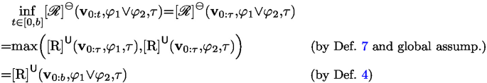
As an instance, we prove $\inf _{t\in [0,b]}{[\mathscr {R}]}^\ominus \left( \textbf{v}_{0:t}, \varphi ', \tau \right) = \mathrm {[R]}^\textsf{U}(\textbf{v}_{0:b}, \varphi ', \tau )$ with $\varphi '=\varphi _1\vee \varphi _2$ as follows. The complete proof is presented in the full version [38].

• First, if $b = \tau$, it holds that:

  

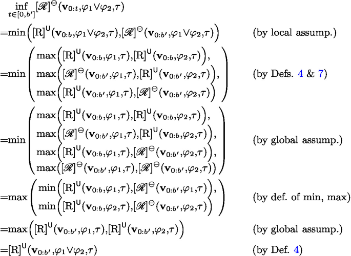
• Then, we make a local assumption that, given an arbitrary b, it holds that $\inf _{t\in [0,b]}{[\mathscr {R}]}^\ominus \left( \textbf{v}_{0:t}, \varphi _1\vee \varphi _2, \tau \right) = \mathrm {[R]}^\textsf{U}(\textbf{v}_{0:b}, \varphi _1\vee \varphi _2, \tau )$. We prove that, for $b'$ which is the next sampling point to b, it holds that,

  

     $\square$

Theorem 3 shows that the result $\mathrm {[R]}^\textsf{U}(\textbf{v}_{0:b}, \varphi , \tau )$ of ClaM can be derived from the result of QCauM by applying $\inf _{t\in [0,b]}{[\mathscr {R}]}^\ominus \left( \textbf{v}_{0:b}, \varphi , t\right)$. For instance, comparing the results of QCauM in Fig. 5 and the results of ClaM in Fig. 2, we can find that the results in Fig. 2 can be reconstructed by using the results in Fig. 5.

Fig. 6.

Refinement among STL monitors

Remark 1

Figure 6 shows the refinement relations between the six STL monitoring approaches. The left column lists the offline monitoring approaches derived directly from the Boolean and quantitative semantics of STL respectively. The middle column shows the classic online monitoring approaches. Our two causation monitors, namely BCauM and QCauM, are given in the column on the right. Given a pair (A, B) of the approaches, $A\leftarrow B$ indicates that the approach B refines the approach A, in the sense that B can deliver more information than A, and the information delivered by A can be derived from the information delivered by B. It is clear that the refinement relation in the figure ensures transitivity. Note that blue arrows are contributed by this paper. As shown by Fig. 6, the relation between BCauM and QCauM is analogous to that between the Boolean and quantitative semantics of STL.

5 Experimental Evaluation

We implemented a tool³ for our two causation monitors. It is built on the top of Breach [15], a widely used tool for monitoring and testing of hybrid systems [18]. Being consistent with Breach, the monitors target the output signals given by Simulink models, as an additional block. Experiments were executed on a MacOS machine, 1.4 GHz Quad-Core Intel Core-i5, 8 GB RAM, using Breach v1.10.0.

5.1 Experiment Setting

Benchmarks. We perform the experiments on the following two benchmarks.

Abstract Fuel Control (AFC) is a powertrain control system from Toyota [27], which has been widely used as a benchmark in the hybrid system community [18,19,20]. The system outputs the air-to-fuel ratio $\texttt{AF}$, and requires that the deviation of $\texttt{AF}$ from its reference value $\texttt{AFref}$ should not be too large. Specifically, we consider the following properties from different perspectives:

• $\varphi ^{\textsf{AFC}}_{1} :=\Box _{[10, 50]}(\left| \texttt{AF}-\texttt{AFref} \right| < 0.1 )$: the deviation should always be small;

• $\varphi ^{\textsf{AFC}}_{2} :=\Box _{[10, 48.5]}\Diamond _{[0,1.5]}\left( \left| \texttt{AF}-\texttt{AFref} \right| < 0.08\right)$: a large deviation should not last for too long time;

• $\varphi ^{\textsf{AFC}}_{3} :=\Box _{[10,48]}(|\texttt{AF}-\texttt{AFref} | > 0.08 \rightarrow \Diamond _{[0,2]}(|\texttt{AF}-\texttt{AFref} | < 0.08))$: whenever the deviation is too large, it should recover to the normal status soon.

Automatic transmission (AT) is a widely-used benchmark [18,19,20], implementing the transmission controller of an automotive system. It outputs the $\texttt{gear}$, $\texttt{speed}$ and $\texttt{RPM}$ of the vehicle, which are required to satisfy this safety requirement:

• $\varphi ^{\textsf{AT}}_{1} :=\Box _{[0,27]}(\texttt{speed} > 50 \rightarrow \Diamond _{[1,3]}(\texttt{RPM} < 3000))$: whenever the $\texttt{speed}$ is higher than 50, the $\texttt{RPM}$ should be below 3000 in three time units.

Baseline and Experimental Design. In order to assess our two proposed monitors (the Boolean causation monitor BCauM in Definition 6, and the quantitative causation monitor QCauM in Definition 7), we compare them with two baseline monitors: the classic quantitative robustness monitor ClaM (see Definition 4); and the state-of-the-art approach monitor with reset ResM  [40], that, once the signal violates the specification, resets at that point and forgets the previous partial signal.

Given a model and a specification, we generate input signals by randomly sampling in the input space and feed them to the model. The online output signals are given as inputs to the monitors and the monitoring results are collected. We generate 10 input signals for each model and specification. To account for fluctuation of monitoring times in different repetitions⁴, for each signal, the experiment has been executed 10 times, and we report average results.

5.2 Evaluation

Qualitative Evaluation. We here show the type of information provided by the different monitors. As an example, Fig. 7 reports, for two specifications of the two models, the system output signal (in the top of the two sub-figures), and the monitoring results of the compared monitors. We notice that signals of both models (top plots) violate the corresponding specifications in multiple points. Let us consider monitoring results of $\varphi ^{\textsf{AFC}}_{1}$; similar observations apply to $\varphi ^{\textsf{AT}}_{1}$.

Fig. 7.

Examples of the information provided by the different monitors

When using the ClaM, only the first violation right after time 15 is detected (the upper bound of robustness becomes negative); after that, the upper bound remains constant, without reporting that the system recovers from violation at around time 17, and that the specification is violated again four more times.

Instead, we notice that the monitor with reset ResM is able to detect all the violations (as the upper bound becomes greater than 0 when the violation episode ends), but it does not properly report the margin of robustness; indeed, during the violation episodes, it reports a constant value of around $-0.4$ for the upper bound, but the system violates the specification with different degrees of severity in these intervals; in a similar way, when the specification is satisfied around after time 17, the upper bound is just above 0, but actually the system satisfies the specification with different margins. As a consequence, ResM provides sharp changes of the robustness upper bound that do not faithfully reflect the system evolution.

Table 1. Experimental results – Average (avg.) and standard deviation (stdv.) of monitoring and simulation times (ms)

We notice that the Boolean causation monitor BCauM only reports information about the violation episodes, but not on the degree of violation/satisfaction. Instead, the quantitative causation monitor QCauM is able to provide a very detailed information, not only reporting all the violation episodes, but also properly characterizing the degree with which the specification is violated or satisfied. Indeed, in QCauM, the violation causation distance smoothly increases from violation to satisfaction, so faithfully reflecting the system evolution.

Quantitative Assessment of Monitoring Time. We discuss the computation cost of doing the monitoring.

In Table 1, we observe that, for all the monitors, the monitoring time is much lower than the total time (system execution + monitoring). It shows that, for this type of systems, the monitoring overhead is negligible. Still, we compare the execution costs for the different monitors. Table 2 reports the monitoring times of all the monitors for each specification and each signal. Moreover, it reports the percentage difference between the quantitative causation monitor QCauM (the most informative one) and the other monitors.

Table 2. Experimental results of the four monitoring approaches – Monitoring time (ms) – $\varDelta A = \nicefrac {(\texttt {QCauM}- A)}{A}$

We first observe that ResM and BCauM have, for the same specification, high variance of the monitoring times across different signals. ClaM and QCauM, instead, provide very consistent monitoring times. This is confirmed by the standard deviation results in Table 1. The consistent monitoring cost of QCauM is a good property, as the designers of the monitor can precisely forecast how long the monitoring will take, and design the overall system accordingly.

We observe that QCauM is negligibly slower than ClaM for $\varphi ^{\textsf{AFC}}_{1}$ and $\varphi ^{\textsf{AFC}}_{2}$, and at most twice slower for the other two specifications. This additional monitoring cost is acceptable, given the additional information provided by QCauM. Compared to ResM, QCauM is usually slower (at most around the double); also in this case, as QCauM provides more information than ResM, the cost is acceptable.

Compared to the Boolean causation monitor BCauM, QCauM is usually faster, as it does not have to collect epochs, which is a costly operation. However, we observe that it is slower in $\varphi ^{\textsf{AFC}}_{3}$, because, in this specification, most of the signals do not violate it (and so also BCauM does not collect epochs in this case).

To conclude, QCauM is a monitor able to provide much more information that exiting monitors, with an acceptable overhead in terms of monitoring time.

6 Related Work

Monitoring of STL. Monitoring can be performed either offline or online. Offline monitoring [16, 30, 33] targets complete traces and returns either $\texttt{true}$ or $\texttt{false}$. In contrast, online monitoring deals with the partial traces, and thus a three-valued semantics was introduced for LTL monitoring [7, 8], and in further for MTL and STL qualitative online monitoring [24, 31], to handle the situation where neither of the conclusiveness can be made. In usual, the quantitative online monitoring provides a quantitative value or a robust satisfaction interval [12,13,14, 25, 26]. Based on them, several tools have been developed, e.g., AMT [32, 33], Breach [15], S-Taliro [1], etc. We refer to the survey [3] for comprehensive introduction. Recently, in [35], Qin and Deshmukh propose clairvoyant monitoring to forecast future signal values and give probabilistic bounds on the specification validity. In [2], an online monitoring is proposed for perception systems with Spatio-temporal Perception Logic [23].

Monotonicity Issue. However, most of these works do not handle the monotonicity issue stated in this paper. In [10], Cimatti et al. propose an assumption-based monitoring framework for LTL. It takes the user expertise into account and allows the monitor resettable, in the sense that it can restart from any discrete time point. In [37], a recovery feature is introduced in their online monitor [25]. However, the technique is an application-specific approach, rather than a general framework. In [40], a reset mechanism is proposed for STL online monitor. However, as experimentally evaluated in Sect. 5, it essentially provides a solution for the Boolean semantics and still holds monotonicity between two resetting points.

Signal Diagnostics. Signal diagnostics [5, 22, 32] is originally used in an offline manner, for the purpose of fault localization and system debugging. In [22], the authors propose an approach to automatically address the single evaluations (namely, epochs) that account for the satisfaction/violation of an STL specification, for a complete trace. This information can be further used as a reference for detecting the root cause of the bugs in the CPS systems [5, 6, 32]. The online version of signal diagnostics, which is the basis of our Boolean causation monitor, is introduced in [40]. However, we show in Sect. 5 that the monitor based on this technique is often costly, and not able to deliver the quantitative runtime information compared to the quantitative causation monitor.

7 Conclusion and Future Work

In this paper, we propose a new way of doing STL monitoring based on causation that is able to provide more information than classic monitoring based on STL robustness. Concretely, we propose two causation monitors, namely BCauM and QCauM. In particular, BCauM intuitively explains the concept of “causation” monitoring, and thus paves the path to QCauM that is more practically valuable. We further prove the relation between the proposed causation monitors and the classic ones.

As future work, we plan to improve the efficiency the monitoring, by avoiding some unnecessary computations for some instants. Moreover, we plan to apply it to the monitoring of real-world systems.

References

Annpureddy, Y., Liu, C., Fainekos, G., Sankaranarayanan, S.: S-TaLiRo: a tool for temporal logic falsification for hybrid systems. In: Abdulla, P.A., Leino, K.R.M. (eds.) TACAS 2011. LNCS, vol. 6605, pp. 254–257. Springer, Heidelberg (2011). https://doi.org/10.1007/978-3-642-19835-9_21
Balakrishnan, A., Deshmukh, J., Hoxha, B., Yamaguchi, T., Fainekos, G.: PerceMon: online monitoring for perception systems. In: Feng, L., Fisman, D. (eds.) RV 2021. LNCS, vol. 12974, pp. 297–308. Springer, Cham (2021). https://doi.org/10.1007/978-3-030-88494-9_18
Bartocci, E., et al.: Specification-based monitoring of cyber-physical systems: a survey on theory, tools and applications. In: Bartocci, E., Falcone, Y. (eds.) Lectures on Runtime Verification. LNCS, vol. 10457, pp. 135–175. Springer, Cham (2018). https://doi.org/10.1007/978-3-319-75632-5_5
Bartocci, E., Falcone, Y. (eds.): Lectures on Runtime Verification. LNCS, vol. 10457. Springer, Cham (2018). https://doi.org/10.1007/978-3-319-75632-5
Bartocci, E., Ferrère, T., Manjunath, N., Ničković, D.: Localizing faults in Simulink/Stateflow models with STL. In: HSCC 2018, pp. 197–206. ACM (2018). https://doi.org/10.1145/3178126.3178131
Bartocci, E., Manjunath, N., Mariani, L., Mateis, C., Ničković, D.: CPSDebug: automatic failure explanation in CPS models. Int. J. Softw. Tools Technol. Transfer 23(5), 783–796 (2020). https://doi.org/10.1007/s10009-020-00599-4
Bauer, A., Leucker, M., Schallhart, C.: Monitoring of real-time properties. In: Arun-Kumar, S., Garg, N. (eds.) FSTTCS 2006. LNCS, vol. 4337, pp. 260–272. Springer, Heidelberg (2006). https://doi.org/10.1007/11944836_25
Bauer, A., Leucker, M., Schallhart, C.: Runtime verification for LTL and TLTL. ACM Trans. Softw. Eng. Methodol. 20(4), 1–64 (2011). https://doi.org/10.1145/2000799.2000800
Ciccone, L., Dagnino, F., Ferrando, A.: Ain’t no stopping us monitoring now. arXiv preprint arXiv:2211.11544 (2022)
Cimatti, A., Tian, C., Tonetta, S.: Assumption-based runtime verification with partial observability and resets. In: Finkbeiner, B., Mariani, L. (eds.) RV 2019. LNCS, vol. 11757, pp. 165–184. Springer, Cham (2019). https://doi.org/10.1007/978-3-030-32079-9_10
Decker, N., Leucker, M., Thoma, D.: Impartiality and anticipation for monitoring of visibly context-free properties. In: Legay, A., Bensalem, S. (eds.) RV 2013. LNCS, vol. 8174, pp. 183–200. Springer, Heidelberg (2013). https://doi.org/10.1007/978-3-642-40787-1_11
Deshmukh, J.V., Donzé, A., Ghosh, S., Jin, X., Juniwal, G., Seshia, S.A.: Robust online monitoring of signal temporal logic. Formal Methods Syst. Des. 51(1), 5–30 (2017). https://doi.org/10.1007/s10703-017-0286-7
Dokhanchi, A., Hoxha, B., Fainekos, G.: On-line monitoring for temporal logic robustness. In: Bonakdarpour, B., Smolka, S.A. (eds.) RV 2014. LNCS, vol. 8734, pp. 231–246. Springer, Cham (2014). https://doi.org/10.1007/978-3-319-11164-3_19
Dokhanchi, A., Hoxha, B., Fainekos, G.: Metric interval temporal logic specification elicitation and debugging. In: MEMOCODE 2015, pp. 70–79. IEEE (2015). https://doi.org/10.1109/MEMCOD.2015.7340472
Donzé, A.: Breach, a toolbox for verification and parameter synthesis of hybrid systems. In: Touili, T., Cook, B., Jackson, P. (eds.) CAV 2010. LNCS, vol. 6174, pp. 167–170. Springer, Heidelberg (2010). https://doi.org/10.1007/978-3-642-14295-6_17
Donzé, A., Ferrère, T., Maler, O.: Efficient robust monitoring for STL. In: Sharygina, N., Veith, H. (eds.) CAV 2013. LNCS, vol. 8044, pp. 264–279. Springer, Cham (2013). https://doi.org/10.1007/978-3-642-39799-8_19
Donzé, A., Maler, O.: Robust satisfaction of temporal logic over real-valued signals. In: Chatterjee, K., Henzinger, T.A. (eds.) FORMATS 2010. LNCS, vol. 6246, pp. 92–106. Springer, Heidelberg (2010). https://doi.org/10.1007/978-3-642-15297-9_9
Ernst, G., et al.: ARCH-COMP 2021 category report: falsification with validation of results. In: Frehse, G., Althoff, M. (eds.) 8th International Workshop on Applied Verification of Continuous and Hybrid Systems (ARCH21). EPiC Series in Computing, vol. 80, pp. 133–152. EasyChair (2021). https://doi.org/10.29007/xwl1
Ernst, G., et al.: ARCH-COMP 2020 category report: falsification. In: 7th International Workshop on Applied Verification of Continuous and Hybrid Systems (ARCH20). EPiC Series in Computing, vol. 74, pp. 140–152. EasyChair (2020). https://doi.org/10.29007/trr1
Ernst, G., et al.: ARCH-COMP 2022 category report: falsification with unbounded resources. In: Frehse, G., Althoff, M., Schoitsch, E., Guiochet, J. (eds.) Proceedings of 9th International Workshop on Applied Verification of Continuous and Hybrid Systems (ARCH22). EPiC Series in Computing, vol. 90, pp. 204–221. EasyChair (2022). https://doi.org/10.29007/fhnk
Fainekos, G.E., Pappas, G.J.: Robustness of temporal logic specifications for continuous-time signals. Theoret. Comput. Sci. 410(42), 4262–4291 (2009). https://doi.org/10.1016/j.tcs.2009.06.021
Ferrère, T., Maler, O., Ničković, D.: Trace diagnostics using temporal implicants. In: Finkbeiner, B., Pu, G., Zhang, L. (eds.) ATVA 2015. LNCS, vol. 9364, pp. 241–258. Springer, Cham (2015). https://doi.org/10.1007/978-3-319-24953-7_20
Hekmatnejad, M., Hoxha, B., Deshmukh, J.V., Yang, Y., Fainekos, G.: Formalizing and evaluating requirements of perception systems for automated vehicles using spatio-temporal perception logic (2022). https://doi.org/10.48550/arxiv.2206.14372
Ho, H.-M., Ouaknine, J., Worrell, J.: Online monitoring of metric temporal logic. In: Bonakdarpour, B., Smolka, S.A. (eds.) RV 2014. LNCS, vol. 8734, pp. 178–192. Springer, Cham (2014). https://doi.org/10.1007/978-3-319-11164-3_15
Jakšić, S., Bartocci, E., Grosu, R., Kloibhofer, R., Nguyen, T., Ničkovié, D.: From signal temporal logic to FPGA monitors. In: MEMOCODE 2015, pp. 218–227. IEEE (2015). https://doi.org/10.1109/MEMCOD.2015.7340489
Jakšić, S., Bartocci, E., Grosu, R., Nguyen, T., Ničković, D.: Quantitative monitoring of STL with edit distance. Formal Methods Syst. Des. 53(1), 83–112 (2018). https://doi.org/10.1007/s10703-018-0319-x
Jin, X., Deshmukh, J.V., Kapinski, J., Ueda, K., Butts, K.: Powertrain control verification benchmark. In: HSCC 2014, pp. 253–262. ACM (2014). https://doi.org/10.1145/2562059.2562140
Koymans, R.: Specifying real-time properties with metric temporal logic. Real Time Syst. 2(4), 255–299 (1990). https://doi.org/10.1007/BF01995674
Leucker, M., Schallhart, C.: A brief account of runtime verification. J. Logic Algebraic Program. 78(5), 293–303 (2009). https://doi.org/10.1016/j.jlap.2008.08.004
Maler, O., Nickovic, D.: Monitoring temporal properties of continuous signals. In: Lakhnech, Y., Yovine, S. (eds.) FORMATS/FTRTFT -2004. LNCS, vol. 3253, pp. 152–166. Springer, Heidelberg (2004). https://doi.org/10.1007/978-3-540-30206-3_12
Maler, O., Ničković, D.: Monitoring properties of analog and mixed-signal circuits. Int. J. Softw. Tools Technol. Transf. 15(3), 247–268 (2013). https://doi.org/10.1007/s10009-012-0247-9
Ničković, D., Lebeltel, O., Maler, O., Ferrère, T., Ulus, D.: AMT 2.0: qualitative and quantitative trace analysis with extended signal temporal logic. Int. J. Softw. Tools Technol. Transfer 22(6), 741–758 (2020). https://doi.org/10.1007/s10009-020-00582-z
Nickovic, D., Maler, O.: AMT: a property-based monitoring tool for analog systems. In: Raskin, J.-F., Thiagarajan, P.S. (eds.) FORMATS 2007. LNCS, vol. 4763, pp. 304–319. Springer, Heidelberg (2007). https://doi.org/10.1007/978-3-540-75454-1_22
Pnueli, A.: The temporal logic of programs. In: FOCS 1977, pp. 46–57. IEEE (1977). https://doi.org/10.1109/SFCS.1977.32
Qin, X., Deshmukh, J.V.: Clairvoyant monitoring for signal temporal logic. In: Bertrand, N., Jansen, N. (eds.) FORMATS 2020. LNCS, vol. 12288, pp. 178–195. Springer, Cham (2020). https://doi.org/10.1007/978-3-030-57628-8_11
Sánchez, C., et al.: A survey of challenges for runtime verification from advanced application domains (beyond software). Formal Methods Syst. Des. 54(3), 279–335 (2019). https://doi.org/10.1007/s10703-019-00337-w
Selyunin, K., et al.: Runtime monitoring with recovery of the SENT communication protocol. In: Majumdar, R., Kunčak, V. (eds.) CAV 2017. LNCS, vol. 10426, pp. 336–355. Springer, Cham (2017). https://doi.org/10.1007/978-3-319-63387-9_17
Zhang, Z., An, J., Arcaini, P., Hasuo, I.: Online causation monitoring of signal temporal logic. arXiv (2023). https://doi.org/10.48550/arXiv.2305.17754
Zhang, Z., An, J., Arcaini, P., Hasuo, I.: Online causation monitoring of signal temporal logic (Artifact). Zenodo (2023). https://doi.org/10.5281/zenodo.7923888
Zhang, Z., Arcaini, P., Xie, X.: Online reset for signal temporal logic monitoring. IEEE Trans. Comput. Aided Des. Integr. Circuits Syst. 41(11), 4421–4432 (2022). https://doi.org/10.1109/TCAD.2022.3197693
Author information
Authors and Affiliations
Corresponding author
Editor information
Editors and Affiliations
Rights and permissions
Open Access This chapter is licensed under the terms of the Creative Commons Attribution 4.0 International License (http://creativecommons.org/licenses/by/4.0/), which permits use, sharing, adaptation, distribution and reproduction in any medium or format, as long as you give appropriate credit to the original author(s) and the source, provide a link to the Creative Commons license and indicate if changes were made.
The images or other third party material in this chapter are included in the chapter's Creative Commons license, unless indicated otherwise in a credit line to the material. If material is not included in the chapter's Creative Commons license and your intended use is not permitted by statutory regulation or exceeds the permitted use, you will need to obtain permission directly from the copyright holder.
Copyright information
© 2023 The Author(s)
About this paper
Cite this paper
Zhang, Z., An, J., Arcaini, P., Hasuo, I. (2023). Online Causation Monitoring of Signal Temporal Logic. In: Enea, C., Lal, A. (eds) Computer Aided Verification. CAV 2023. Lecture Notes in Computer Science, vol 13964. Springer, Cham. https://doi.org/10.1007/978-3-031-37706-8_4
Download citation
DOI: https://doi.org/10.1007/978-3-031-37706-8_4
Published:
Publisher Name: Springer, Cham
Print ISBN: 978-3-031-37705-1
Online ISBN: 978-3-031-37706-8
eBook Packages: Computer ScienceComputer Science (R0)