
Abstract
The ultimate aim of radiobiological research is to establish a quantitative relationship between the radiation dose absorbed by biological samples (being this a cell, a tissue, an organ, or a body) and the effect caused. Therefore, radiobiological investigations need to be supported by accurate and precise dosimetric measurements. A rigorous standardized methodology has been established to assess and quantify the radiation dose absorbed by biological samples and these will be reviewed and discussed in this chapter. Dosimetric concepts at the macro- and microscopic levels are discussed with a focus on key physical quantities, their measurement technologies, and the link to the biological damage and response. This chapter will also include a description of state-of-the-art irradiation facilities (e.g., mini- and micro-beams) used for probing mechanisms underpinning radiobiological responses. Finally, the link between energy deposition events and detectable biological effects (from the molecular to the organism level) is investigated using Monte Carlo simulation codes and macroscopic radiobiological models.
Fabiana Da Pieve is currently employed by the European Research Council Executive Agency, European Commission, BE-1049 Brussels, Belgium. The views expressed are purely those of the authors and may not in any circumstances be regarded as stating an official position of the European Commission
You have full access to this open access chapter, Download chapter PDF
Keywords
FormalPara Learning Objectives-
To understand the concept of dose and the notion of energy deposition and energy transfer.
-
To learn the working principles of the main types of detectors used for radiation dosimetry.
-
To understand how the dose is measured in micrometric volumes and what the importance of microdosimetry is in radiobiology.
-
To understand how early DNA damage is generated by ionizing radiation.
-
And how this can be simulated using Monte Carlo (MC) track structure codes.
-
To get an overview of the state of the art of the mechanistic simulation and the DNA damage scoring methods.
-
To get to know micro-beams and mini-beams, their production and use, and why they are important for radiobiological research.
-
To understand the underlying assumptions and derivation of target theory, which is the basis for all stochastic dose-response models at molecular and cellular level.
-
To learn about the linear quadratic model, the strengths and limitations of the model as well as the different interpretations of the model with respect to the underlying biology.
-
To understand the difficulties in modeling stochastic effects for whole organisms and for different dose rates.
4.1 Principles of Radiation Dosimetry
4.1.1 Energy Deposition and Transfer
4.1.1.1 Fluence
Particle fluence, or planar fluence, Φ, is defined as the number of ionizing particles which traverse a finite plane in space some distance from the source. If dN particles are incident on a planar surface of area, dA, then the fluence is Φ = dN/dA [1, 2].
We may also define the energy fluence, Ψ, which is the radiant energy, dR, which crosses a plane of area, dA, as Ψ = dR/dA. The radiant energy, R, of a radiation field is defined as the total energy of the particles that cross the plane, excluding their rest mass energy. The fluence rate may be defined in terms of energy fluence or planar fluence and is simply the rate at which either energy fluence or planar fluence cross unit area. In the context of the amount of radiant energy absorbed in matter, these concepts provide the basis from which all the remaining dosimetric quantities are defined [1, 2].
4.1.1.2 Exposure
Exposure, X, is defined as the total charge which is liberated per unit mass in air by ionizing radiation [1, 2]. Its unit is the Roentgen, R, where one Roentgen is 2.58 × 10⁻⁴ C kg−1. Exposure is related to energy fluence, Ψ, by the following equation:
where (μen/ρ)air is the mass energy absorption coefficient of air which defines the fraction of the energy of a beam of particles which is absorbed per unit mass of air at a particular beam energy. Wair = 33.97 eV is the energy required to produce an ion pair in air and e is the charge of the electron.
4.1.1.3 Kerma
Kerma, K, is defined as the kinetic energy released per unit mass of material by a specific combination of an incident radiation field and an absorbing material. Kerma is related to energy fluence, Ψ, by the following equation:
where μtr/ρ is the mass energy transfer coefficient, which defines the fraction of the incident radiant energy which is released as kinetic energy in charged particles in a given volume of material. More strictly, the Kerma is the amount of energy liberated through ionization in the volume encompassed by a unit mass of an absorbing material [1, 2]. This energy is transferred through ionization of the material at the atomic level and is ultimately manifested in the kinetic energy of ionization electrons in the material. As may be seen from Fig. 4.1, kinetically charged particles or photons, created in collisions between incident ionizing particles and the material, may not deposit their energy in the mass volume. Therefore, Kerma is a measure of the amount of ionizing energy offered for absorption in the material, which in this case is the initial kinetic energy of the primary electron.

Kerma in relation to interactions between ionizing photons and matter in a unit mass volume
4.1.1.4 Energy Imparted
The energy imparted, ϵ, by ionizing radiation to the matter in a volume is given by the following equation [3]:
where the first and second terms in the equation, respectively, describe the sums of all the radiant energies of all ionizing radiations entering and leaving a particular volume. The third term denotes the sum of all the mass energies of all the particles produced during the interactions of the ionizing radiations with the matter to which it is imparting energy. In diagnostic radiology, the photon energy is not sufficient to instigate pair production (production of positrons and electrons in the vicinity of a strongly positive nucleus), and therefore particle production does not occur. Thus, for diagnostic energies, the third term on the right-hand side of Eq. (4.3) is zero [1, 4]. Energy Imparted is quoted in the units of energy, the Joule, J.
A distinction must be made between the term “Energy Imparted” and the term “Imparted Energy.” Energy Imparted is the term for a gross quantity or concept, where the energy is imparted to matter that has a macroscopic size. Imparted Energy is the energy that is imparted in a single interaction between any particle and the matter in a given volume. The Imparted Energy, dϵ, in an interaction is a stochastic quantity, and is difficult to measure, and impossible to infer with any great accuracy [3, 5]. Thus, the Energy Imparted is also a stochastic quantity. However, repeated measurements can establish mean energy imparted, \( \overline{\varepsilon} \), which is a non-stochastic quantity (Box 4.1).
Box 4.1 Dosimetry Quantities: Kerma and Exposure
-
Kerma, K, is defined as the kinetic energy released per unit mass of material by a specific radiation field and it is related to energy fluence, ψ
-
Exposure, X, is defined as the total charge which is liberated per unit mass in air by ionizing radiation. Its unit is the Roentgen, R.
4.1.2 Absorbed Dose
The absorbed dose (sometimes referred to simply as “dose”) is the radiant ionizing energy absorbed per unit mass of absorbing material. It is therefore defined as:
The quantity ε/m is sometimes referred to as the specific energy. It is stochastic in the same way that the imparted energy in a given interaction is stochastic, but with repeated measurements, and on macroscopic scales involving many single particle interactions, it becomes a measurable quantity ([1], p. 86; [2, 4]). The unit of Absorbed dose is the Gray, Gy, which is equal to J kg−1.
The Kerma in Eq. (4.2) may be split into two parts depending on the ways in which the energy of the photon is lost through interactions with the material [1]. Photons may either release their energy through collision interactions in which excitation and ionization of the stopping material occur or through radiative processes in which their energy is radiated through the release of photons. Thus, the Kerma can be expressed as:
where Kc is the portion transferred through collisions, and Kr is the portion transferred through radiative interactions [1]. Radiative interactions generally occur in situations in which charged particles are incident on a material [1]. In the case of diagnostic radiology, Kerma is released through collision interactions, with Collision Kerma therefore given by:
In diagnostic radiology, a simple relationship between Kerma and Absorbed dose may be derived. When charged particle equilibrium (CPE) exists in a medium, the number of charged particles leaving a unit mass volume is replaced by an equal number entering from other mass volumes. In such a situation, which occurs at the photon energies in diagnostic radiology, all Kerma is absorbed in the unit mass volume. It has been shown by Attix, that for a medium of uniform density and atomic composition, such a situation does indeed exist for a field of X-ray photons and a uniformly irradiated medium [1, 2]. In this case the Absorbed dose, D, and Collision Kerma, Kc, are equal, such that
Box 4.2 Dosimetry Quantities: Absorbed Dose
-
The Absorbed Dose is the energy absorbed per unit mass of material. The unit of Absorbed Dose is the Gray, Gy, which is equal to J kg−1
4.1.3 Radiation Detectors
In general, radiation detectors operate by providing the means to measure the energy deposited over time in the detector absorbing material from exposure to a source of ionizing radiation. This is typically measured as the quantity of charge, Q, over time elicited from an absorbing medium forming the main component of the detecting element. An ideal radiation detector is one that gives spatial resolution, temporal resolution, information regarding the energy of the particle, and information regarding the identity of the radiation. In reality, single detectors of this type are difficult to construct such that practical detectors that are used in the field have a focused range of capabilities which should be taken into consideration when a detector is chosen for a particular application [6, 7].
4.1.3.1 Ionization Chambers
Ionization chambers are designed to measure the number and/or total energy deposited as a result of the ionizations produced when a charged particle or ionizing photon traverses the detector medium. Therefore, they are not suitable for the detection or analysis of neutral particles. Ionization detectors consist of an isolated detection medium, generally a gas such as air that can be easily ionized (i.e., has a low ionization potential), which is placed between two oppositely charged electrodes (Fig. 4.2). The medium should be chosen such that it does not respond adversely to ionization such that its characteristics will not change with use.

Schematic of the basic elements of an ionization detector
The charged particle will ionize the detector medium along its path and these ions will then be accelerated towards the detector electrodes. In general, a high electric field is applied between the electrodes to prevent the recombination of ions produced by the traversal of the charged particle. As the charged particle traverses the sensitive region of the detector (i.e., the gas) it produces multiple electron-ion pairs, which begin to drift along the electric field lines and reach the plates of the detector. These ions may produce further ionization of the neutral gas atoms via further collision, ultimately producing a small current that induces a voltage drop across the resistor. These chambers typically generate very low measurement currents per ionizing particle, and therefore require low noise amplifiers to improve their operating performance.
The amplified output signal from the detector may be used to trigger a counting mechanism to measure the number of incident charged particles or ionizing photons (i.e., exposure) or its pulse height may be analyzed to determine the total energy within the beam (i.e., dose). The amount of ionization that is detected is dependent on the nature of the gas used in the detector, the level of the applied electrical field, and the characteristics of the plates used in the detector. How the chambers operate, i.e., as a device for the measurement of absolute energy deposition or number of charged particle incident on the detector, depends on the HV level applied to the detector, as depicted in Fig. 4.3 [7].

Signal response to ionization as a function of the applied voltage for heavily ionizing (top curve) and weakly ionizing particles (lower curve). In the Geiger region, the output does neither depend on the voltage nor on the amount of deposited energy or initial ionization. [Adapted from Fig. 4.12 Martin and Shaw (2006). Copyright (2006), Wiley Publishers]
When the applied voltage is small, the electrons and ions can recombine soon after they are produced and only a small fraction of the ions reach their respective plates in the detector (Fig. 4.3). As the applied voltage between the plates is increased, a region is reached where the output pulse reflects the amount of ionization seen in the chamber (Ionization region). When the voltage is increased still further, the electrons and positive ions released by the initial ionization can themselves cause further ionizations in the medium and thus amplify the ionization pulse (Proportional region). Increasing the applied field still further (Geiger region) creates an avalanche effect and a highly amplified output signal. Any further increases in the applied voltage lead to a continuous discharge of the detector [6].
It is possible to determine the typical output current that will be generated by an ionization chamber in the presence of a source of known activity. Consider the case of an in-air ionization chamber (where air has an ionization potential of 30 eV) which is exposed to alpha particles (Eα = 5.486 MeV) from a 10 MBq Am-241 source. The total number of ionizations produced by a single Am-241 α-particle will be the ratio of the energy of the alpha particle to the ionization potential of air:
In this case, the total number of ionizations produced will be the product of the activity of the source and the number of ionizations produced by a single alpha particle, or N = 1.829 × 10¹² ionizations, which are observed in a single second (as the unit of activity, the Bq is s−1 in SI units). The final step is then to compute the product of the total number of ionizations with the charge on the electron such that the total current observed will be:
Frequently, ionization chambers are open to the air to allow for changes in ambient pressure which could collapse or expand a sealed chamber, damaging the thin chamber walls. As a consequence, chamber outputs must be adjusted for changes in ambient temperature, T, and pressure, P, from those at which the chamber was calibrated, Tn and Pn, respectively. In practice, we can multiply the chamber output by the following correction factor to adjust for ambient conditions (where all temperatures are expressed in Kelvin and pressures in Pascals [6]):
4.1.3.2 Proportional Counters
While the ionization chamber provides a device for the measurement of absolute energy deposition, it does not provide information on directionality. Proportional counters are ionization chambers that may be used for both measuring absolute energy deposition (through a measurement of the pulse height) in addition to giving directional information on the path of charged particle (through the output of a given anode wire, each of which is independently amplified).
Multi-wire proportional chambers (MWPCs) such as those shown in Fig. 4.4 are used in high-energy particle physics experiments as a means of tracking the path of charged particles. Anode wires (typically with a ~2 mm separation) are positioned between the cathode plates of the chamber (which have a typical separation of 1 mm) and the construct is sandwiched between thin mylar windows or some other superstructure, with an operating gas infused into the region between the plates. In practice, several individual chambers may then be joined together to provide fine detail on the direction of passage of individual charged particle, where pulses will be produced on the anode electrodes closest to the path of the charged particle through the detector as a result of ionization of the gas in the region closest to each anode. MWPCs can be used to infer further information on the momentum of beams of charged particles via the degree of their deflection in a magnetic field (which is typically how they have been used in collider experiments such as the LHC at CERN [6]).

4.1.3.3 Scintillators and Photomultiplier Tubes
Scintillators are materials that react to the passage of a charged particle by the emission of a very small flux of photons of light. Charged particles may excite electrons within atoms of the scintillating material to a higher energy state; these atoms then emit photons as they de-excite to their ground state. Scintillators can be developed from organic (e.g., naphthalene or anthracene) or inorganic (including sodium iodide or cesium iodide) materials and have applications as the first detection element with gamma cameras used in nuclear medicine.
Scintillating materials typically need to be chosen to detect photons of a specific wavelength and may often be doped to achieve specific wavelength sensitivity. They are generally coupled to photomultiplier tubes (PMT) to amplify the intensity of the weak photon signal output from the scintillator, either for photon counting or imaging applications.
In Fig. 4.5, a schematic of a photomultiplier tube is shown. An incoming charged particle or ionizing photon impacts the scintillator, which emits a photon flux towards a photocathode material (constructed typically with a negatively charged plate covered by a photosensitive material such as gallium–arsenide or indium–gallium–arsenide). Here, the photon flux is converted to an electron flux as they enter the inner (evacuated) environment of the PMT tube. These electrons are accelerated towards the first of several dynodes by the high-voltage field between the photocathode and the anode. When each electron collides with a dynode, it causes the emission of several electrons (typically 5–10), which are then accelerated towards subsequent dynode and amplify the electron flux through collision and reemission. At the detector anode, a significant and measurable electric current is then generated as a result of the acquisition of a single photon. Apart from a small degree of signal fluctuation, the current seen at the anode is linearly proportional to the photon flux seen at the photocathode [6, 7].

Schematic diagram of a photomultiplier tube (PMT) (courtesy of Physics Libretexts, Fig. 31.2.3)
4.1.3.4 Semiconductor Detectors
Semiconductor detectors based upon p–n junction diodes offer a practical and robust option for detector construction, operating in a similar manner to an ionization chamber [6, 7]. Here a p–n junction is constructed through the joining together of a piece of p-type semiconductor (such as silicon or germanium) to a piece of n-type silicon. P-type material is doped with atoms of a material with one vacant outer-electron state, such as boron, B, while N-type material is doped with atoms of a material with an extra “free” electron in its outermost energy level, such as antimony, Sb. At the junction between the two materials a “depletion layer” is formed where electrons from the N-type material migrate to the P-type material to fill vacant energy states or “holes” leaving behind holes in the N-type material surrounding the junction. This creates a region where electrons and holes are depleted around the junction and creates a barrier to conduction. For the purposes of photon or particle detection, the depletion region is the sensitive portion of the electronic detector. When operated in reverse bias (Fig. 4.6a, b), this depletion region is larger and these detectors are typically operated in reverse bias with a voltage of 100 V to increase the depletion layer and therefore the sensitive region of the detector [6, 7].

(a) Schematic of a p–n junction diode operated in forward and reverse bias. (b) Operating characteristics of the diode in forward and reverse bias
When the sensitive element of the detector is exposed to a charged particle or ionizing photon, this causes electrons within the depletion layer to be promoted from the valence band to the conduction band (Fig. 4.7), and their conduction through the junction towards the positive terminal of the detector. Here, the valence band is equivalent to the energy level of the outermost electron, while the conduction band is the energy level of the next vacant energy state above the valence band. A current is produced which is proportional to the energy loss by the charged particle or photon within the depletion layer [6, 7]

Operation of a semiconductor particle detector (a) where an incident proton causes the promotion of one or more electrons from the valence to the conduction band within the detector (b)
The creation of an electron–hole pair in a silicon or germanium semiconductor requires as little as ~3 eV in comparison to the 30 eV required for in-air ionization chambers. Detectors can be constructed and tuned to radiation of a specific wavelength, λ, by altering the energy difference between the valence and conduction bands, or the band gap, Egap, as shown in Fig. 4.7 and Table 4.1.
Semiconducting materials, when incorporated in radiation detectors can therefore produce a large signal in response to irradiation with a small photon flux. The detectors can be constructed very thinly (as little as 200–300 μm) for the detection of ionized particles, or larger for stopping of photons. Their performance is approximately linear if an electric field is applied that prevents the recombination of the electrons and holes formed by the radiation [6, 7].
4.1.3.5 Cerenkov Detectors
The phenomenon of Cerenkov radiation was first observed and described by Pavel Cerenkov in 1934 and characterized by Franck and Tamm in 1937. This work resulted in all three being given the Nobel Prize in physics in 1958.
To understand the operation of Cerenkov detectors we must first describe the effect itself. Suppose that we have a charged particle traveling at a relatively low velocity though a static medium. As the particle travels slowly relative to the speed at which the ions/molecules of the material can orient and reorient themselves as it passes, the ions/molecules will orient themselves such that the part of the ion/molecule that is charged opposite to the charge of the ionizing projectile would be in the direction of the particle (Fig. 4.8a). The molecules are displaced in an isotropic conformation relative to the position and direction of movement of the charged particle, and therefore there is no overall change in the energy of the medium locally [6, 7].

(a) Passage of a charged particle through a medium of refractive index n at velocities that polarize the medium. (b) The generation of coherent light waves via the Cerenkov effect. (c) The formation of a cone of Cerenkov light along the path of the charged particle through a medium with positive and (d) negative refractive index. [Taken from Shaffer et al., Nature Nanotechnology, 12, 106–117 (2017). Copyright Springer Nature]
However, in instances where the velocity of the particle, v ~ c/n or v > c/n, the molecules of the medium that are displaced by the passage of the charged particle are generally anisotropic relative to the position and diNurUhr (Fig. 4.8b). By Huygens principle of wavelets, each of the reoriented molecules of the medium can reradiate the energy delivered to them and do so as point wavelet sources. These sources will be coherent along a direction as shown in Fig. 4.8c. If ϑ is the angle at which the point sources reradiate, then it may be shown that
where n is the refractive index of the medium and β = v/c, where v is the velocity of the particle and c is the speed of light.
It is therefore possible to discriminate the identity of high energy charged particles purely based on the angle of Cerenkov emission or the threshold value of n at which Cerenkov emission is observed [6, 7]. In particle physics, experiments materials of various refractive indices are typically used to provide several potential Cerenkov thresholds for the detection of a variety of radiation types. The weak Cerenkov photons can be detected using PMTs or electronic photodetectors. Cerenkov photons are also observable as a result of the passage of charged particles through human tissue and Cerenkov imaging has seen a recent application for in vivo dosimetry in radiotherapy [8].
4.1.3.6 Calorimeters
Calorimeters allow the estimation of the total energy of a high-energy charged particle or ionizing photon through absorption of its total energy, via successive ionization of the material in the detector in a process that is termed a particle shower (Fig. 4.9), in a detector that is capable of absorbing all of the particles incident radiation. These devices may be ionization chambers as described earlier or semiconductor detectors, or a combination of the two. Depending on the nature and identity of the incident particle, it can create ionizing photons through bremsstrahlung or can produce further “hard” ionizing particles that may not be stopped easily in detectors with unsuitable absorbing characteristics, and therefore a single detector type will not achieve the experimental objectives (Box 4.3).

(a) A particle shower within a calorimeter; (b) a particle shower caused by the incidence of a photon on a calorimeter
Box 4.3 Radiation Detectors
-
Radiation detectors measure the energy deposited over time in the detector-absorbing material
-
An ideal radiation detector provides spatial resolution, temporal resolution, information regarding the energy of the particle, and information regarding the identity of the radiation. No single detector can offer these simultaneously
-
Ionization chambers are common dosimeters that measure the ionizations produced when a charged particle or ionizing photon traverses the detector medium (generally a gas, requiring temperature and pressure corrections). An electric field is applied between the electrodes to prevent the recombination of ions produced.
-
Proportional counters are ionization chambers that also provide directional information on the path of charged particles
-
Scintillator materials are also used as dosimeters by relating the flux of photons emitted to the energy deposited. They are generally coupled to photomultiplier tubes (PMT) to amplify the intensity of the photon signal
-
Semiconductor detectors measure the number of charge carriers produced by the radiation in the detector material. Semiconductor materials are used due to the small energy required to produce electron-hole pairs
-
Cerenkov detectors record light produced by charged particles traveling through materials at a velocity greater than that at which light can travel through the material
-
Calorimeters quantify the absolute dose absorbed by measuring the increase in temperature produced by radiation
4.1.4 Monte Carlo Methods
The Monte Carlo (MC) method is a numerical calculation method based on random draws. A succession of draws is carried out in order to sample the random variables of the treated problem to deduce a value of interest. Repeated several times, this procedure allows to obtain a distribution of the values of interest and thus an estimation of their mean and their associated confidence interval. However, the number of samples must be sufficiently large for the empirical mean of the results to be an unbiased estimator of the expectation of the quantity of interest and its distribution as predicted by the central-limit theorem. In this process, the quality of the random number generator is essential. However, only pseudo-random numbers (having a period) can be generated and each Monte Carlo calculation code uses a different mathematical algorithm for that purpose.
The Monte Carlo method is currently used in many fields of physics to model the interactions of particles in a medium. In particular, it is used in dosimetry to estimate the energy loss of the particles in the medium and thus the absorbed dose.
To simulate the course of the particles, MC codes use the notion of cross-sections expressed in barn (b) (1 barn = 10−22 cm2). This cross-section is a physical quantity representing the probability of collision between an incident particle and a target, as it is proportional to the ratio between the interaction rate (T) and the incoming particle fluence (φ):
with Ntarget the number of target particles in the target volume, corresponding to the surface S of the beam intercepting the target and starget the number of target particles per surface unit.
Therefore, we can calculate the probability p for a particle to interact with the target in the following way:
With NA the Avogadro’s constant, ρ the target medium density, d the target thickness, and A the atomic mass of the target medium. Sigma?
We see that the probability of interaction depends directly on the quantity (ρ ⋅ d), which has the unit of g cm−2. Moreover, we see the unit of σ: p appear without dimension, σ has the dimensions of a surface. One can imagine σ as a geometrical surface: a particle striking the target in this area would interact, while outside this area it would cross the target without diffusion (Fig. 4.10).

Schematic representation of the cross-section for a target with Ntarget = 9 and an irradiated surface S
From this concept of interaction cross-section, it is possible to define the mean free path (λ) of a particle by means of the equation:
This mean free path corresponds to the average value of a random variable representing the path traveled by a particle between two interactions (l). The probability density of this random variable is given by: \( p(l)=\frac{1}{\lambda }{e}^{-l/\lambda } \). This probability density allows to sample the distance traveled by a particle between two interactions using a random variable ξ0 uniformly distributed between 0 and 1 as follows l = − λ ln ξ0.
Cross-sections used in the MC codes are obtained either experimentally or are calculated from theoretical diffusion models and then used to determine the probability distributions of the random variables related to a trajectory as mean free path but also the type of interaction or the energy loss.
A key point of these MC calculations is related to the simulation of the electron (and positron) interactions. Indeed, these particles lose a very small part of their energy at each interaction they undergo. Thus, they generate a very large number of events before being finally absorbed into the medium. The detailed simulation of this cascade of interactions and of these weak energy deposits is particularly slow. Thus, most Monte Carlo codes apply simplifying theories called “condensed histories” or “multiple scattering” that summarize a certain number of interactions in a single step, allowing to reduce the simulation time. The compromise between the detail of the simulation and the speed of the calculation conditions the performance of the calculation code. Among the most used MC codes in dosimetry, we can highlight PENELOPE « Penetration and ENErgy LOss of Positrons and Electrons, EGSnrc « Electron Gamma Shower », MCNP6 and MCNPX « Monte-Carlo N-Particle eXtended », or Geant4 « GEometry And Tracking » [9,10,11,12,13].
Thanks to their capacity to include a large part of the physical processes involved in radiation–matter interactions and the possibility of taking into account all the different components of the experimental geometry of the problems, MC codes have clear advantages since they can provide information on the values of certain quantities that cannot be determined experimentally.
In radiotherapy, it is required to deliver a dose to the tumor with an uncertainty equal to or less than 5% [14]. Prescribed dose metrology involves the determination of quantities characterizing the transfer and absorption of energy in the irradiated media. In principle, Monte Carlo simulations allow the dose calculation with the required accuracy using phantoms or even patient’s voxelized images and thus provide information on dose distribution in the organ volume. However, to do this it is necessary to have quite exact knowledge of the beam characteristics, which means the need for detailed consideration of each accelerator including head shielding and structural components, which is very time-consuming and often submitted to industrial secret. Therefore, up to now, Monte Carlo codes have been mainly used to calculate the correction factors, often close to unity, to be applied to the experimental values obtained at the hospital during this metrological control.
Nevertheless, The Monte Carlo technique is increasingly used for clinical treatment planning by implementing MC-based algorithms that are used in situations where conventional analytical methods used by the Treatment Planning Systems (TPS) of the machines are not enough. To decrease the computation time, most implementations for radiotherapy divide the calculation into two steps. The first one consists in simulating the head of the treatment machine. This part being fixed and independent of the ballistics associated with the treatment of patients, a phase space can be recorded at the output of the treatment head and be reused. The second step consists in tracking the particles previously recorded in the phase space in the specific geometry of a patient for a specific treatment. Both parts must be, of course, experimentally verified by comparisons with percentage depth dose curves (PDD) and absorbed dose profiles at various depths in water or with measurements in situations where electronic equilibrium is not respected, for example, at the interfaces of materials of different densities (Box 4.4).
Box 4.4 Monte Carlo Simulation Method
-
The Monte Carlo (MC) method is a numerical calculation method used to estimate the dose deposited through simulation of the stochastic events through which radiation deposits energy
4.2 Radiation Microdosimetry
Microdosimetry was first introduced by H.H. Rossi in 1955 and is a fundamental and evolving research field in experimental radiation science [15, 16]. It studies the interaction between radiation and matter in micrometric volumes of cell-like dimensions taking into account the stochastic nature of the energy deposition process.
4.2.1 Definition, Concepts, and Units
The interaction between radiation and matter is a stochastic process that manifests itself as energy deposition, δ-electron production, or nuclear reactions. The latter produce charged particles, called secondaries, which in turn interact with surrounding matter, releasing energy, as δ-electrons do. The fundamental quantity in microdosimetry is the lineal energy, y, which aims to quantify the individual energy deposition events. Energy deposition is a stochastic quantity defined as the energy deposited at the point of interaction:
where Tin is the energy of the incident ionizing particle (exclusive of rest mass), Tout is the sum of the energies of all ionizing particles leaving the interaction site (exclusive of rest mass), and QΔm is the change of rest mass energy of the atom and all particles involved in the interaction. εi is usually expressed in eV. The lineal energy, y, is therefore defined by the ICRU report 36 ([17], p. 36) as the quotient of εtot by l, where εtot is the total energy imparted to a volume of matter by a single energy deposition event and l is the mean chord length in that volume:
The lineal energy is usually expressed in keV/μm. A single energy deposition event denotes the energy imparted by correlated charged particles. Due to the stochastic nature of radiation interaction, each particle traversal gives rise to a different lineal energy value thus producing a probability distribution function. Such probability distribution functions fully characterize the irradiation at a given point. The individual energy deposition events (opportunely corrected for the detector charge collection efficiency and converted into energy to tissue equivalent material) are collected in a form of spectrum [f (ε) vs ε] where f (ε) is the probability of an energy deposition event ε. From these energy spectra, the lineal energy spectra [f (y) vs y; with y = lineal energy] can be calculated by dividing the energy events by the average chord length of the detector, which is the average distance that the particle will traverse in the detector. In the case of a spherical detector, this can be demonstrated to be 2/3 of the diameter, while for thin plate detectors in a unidirectional particle beam, this can be approximated to the detector thickness [18]. The probability density function f (y), also called lineal energy frequency distribution, is independent of the absorbed dose or dose rate. Its expectation value \( \overline{y} \)F is called frequency mean lineal energy and, being a mean value, is no longer a stochastic quantity.
As the radiation biological damage is proportional to the dose delivered, it is useful to consider also the lineal energy dose distribution d (y), as it provides the fraction of the total absorbed dose in the interval [y, y + δy]. The dose-weighted lineal energy distribution d (y) is therefore given by:
By definition, this distribution is normalized and is generally plotted as d (y) vs log (y) to make it easier to appreciate the relative contribution of various energy deposition events (see Fig. 4.11).

The same microdosimetric spectrum represented through the raw counts per channel acquired (a), counts as a function of the lineal energy (y) after a channel calibration (b), converted into lineal energy frequency (c) and dose (d) distributions
Similar to the frequency mean lineal energy \( \overline{y} \)F, the dose-weighted mean lineal energy \( \overline{y} \)D can be defined as
This quantity provides the average lineal energy value when each energy deposition event is weighted based on its contribution to the total dose.
A crucial parameter for the calculation of the lineal energy is the mean cord length (\( \overline{l} \)), as the energy lost by a charged particle traversing a finite volume is proportional to the path traveled (track length) in that volume. The cord length however is itself a random quantity and for microdosimetric calculations, its mean can be estimated through Monte Carlo simulations or, for convex volumes, using the Cauchy formula \( \overline{l} \) = 4 V/S where V is the body volume and S is its surface area.
4.2.2 Technologies and Detectors
The first microdosimeter detector was designed and developed by Rossi in 1955 [16]. It was a spherical proportional counter made of tissue-equivalent plastic walls and filled with low-pressure tissue-equivalent gas (TEPC—Tissue Equivalent Proportional Counter). The low pressure allows to simulate micrometer volumes using a millimeter-size chamber (10–150 mm diameter), which is easier to handle and manufacture. Methane or propane-based gases are typically used at a pressure of ~0.9 kPa to simulate volumes of a few micrometer in diameter. The electrons produced by the traversal of the radiation through the chamber are amplified and collected by an electric field. Every radiation traversal generates therefore a small current that gives rise to a pulse later processed by the acquisition electronics. This allows the quantification of the energy deposited in micrometer volumes by individual radiation events. TEPCs are still the most common detector for microdosimetry measurements. Their main limitation is related to the wall-effects, which are events generated by the interaction of the incoming radiation with the walls of the device, and to controlling the electron avalanche process caused by high electric fields, which are required to simulate very small volumes. New devices are addressing these limitations with wall-less TEPC where specially designed electrodes are aligned to generate an electric field within a confined volume and reduce electron avalanches (avalanche confinement TEPCs). The new devices are also less cumbersome than the first TEPC designed by Rossi and can be operated in clinically relevant radiation beams.
More recently, solid-state detectors have been employed as microdosimeters taking advantage of their unique characteristics including compact size, economic development, and low sensitivity to vibrations, which makes them particularly suitable for clinical environment. The working principle is based on the electron-hole pairs produced by the radiation as it crosses the sensitive volume of the semiconductor crystal. The number of electron-hole pairs is proportional to the total energy deposition (ΔE) and the crystal ionization energy (W; average energy required to produce an electron-hole pair) by
The ionization energy is specific for each crystal and in the order of a few eV for typical semiconductor materials, which is an order of magnitude lower than that required for gas detectors. Furthermore, it is largely independent of the energy of the incoming radiation. Similar to TEPCs, the current generated by the collection of the produced electrons is used to quantify the energy deposition events. As the sensitive volume of the detector can be of a few micrometers, the pulses generated provide a microdosimetric spectrum of the incident radiation. In order to serve as a microdosimeter, solid-state detectors need to have well-defined and micrometer-sized sensitive volumes coupled to an efficient charge collection mechanism, as the electrical signal generated can be very small. A potential drawback of solid-state microdosimeters is their non-tissue equivalence, which generally requires additional conversion calculations provided by Monte Carlo simulations.
Silicon and diamond microdosimeters have been realized with sensitive volumes as low as 1 μm in thickness and a few hundred μm2 area and collection charges approaching 100%. Their small geometry provides also high-spatial resolution and the possibility to measure full therapeutic beam intensities, as the electronic chain is not saturated by the large number of particles required for clinical use. A main limitation of semiconductor microdosimeters is the electronic noise, as the devices work with little or no electronic gain due to the small voltage that can be applied to the small-volume semiconductor. This limits the lowest energy events that can be detected. The fixed size of the crystal also implies that different detectors may need to be used to obtain microdosimetric information for different sensitive volumes while gas-based detectors can achieve this by varying the gas-pressure. The advantages and disadvantages of both detector types are confronted in Table 4.2.
4.2.3 Biological Relationship Response
In the framework of radiation biology, either the linear energy transfer LET or the lineal energy can be used to specify the radiation quality. While the LET is frequently used, at least for broad classifications of different radiation qualities (high vs low LET, i.e., densely vs sparsely ionizing radiation), the use of the lineal energy is less common due to the limited experimental data and the complexity in analyzing the microdosimetric spectra. However, the use of LET to determine radiation quality is affected by some intrinsic limitations such as different particles of different mass and energy having the same LET being still characterized by a different energy distribution of the secondary electrons. In general, the microdosimetric spectra provide information that is not captured in the LET and it may be very beneficial for fundamental radiobiological studies aimed at linking biological response to energy deposition events, as well as for radiation protection and clinical work, e.g., predicting treatment efficacy.
Several LET-based RBE models have been developed over the years. The Microdosimetric Kinetic Model (MKM) is a model based on the dual radiation action theory and specifically developed to link microdosimetric measurements to radiobiological effects [19]. The central hypothesis of the dual radiation action theory is that the number of lethal lesions is, through a linear quadratic relationship, proportional to the specific energy deposited in a microscopic site. The specific energy (z) is defined as the ratio between the energy imparted (ε) and the mass of the microscopic volume (m) [17]:
As both the specific energy (z) and the lineal energy (y) measured by microdosimetry are related to a microscopic volume, the two quantities are linked through the microscopic volume mass (m) and mean chord length (l):
with l, m, ρ, and rd the mean chord length, the mass, the density, and the radius of the microscopic volume, respectively.
Kase et al. [20] formalized the link between cell survival fraction SF and the microdosimetric measurements:
with
where α0 and β0 are the linear quadratic parameters specific for each cell line (usually taken from X-ray measurements), D is the macroscopic dose absorbed by the cell and ρ is the cell density. y0 and rd are fixed parameters accounting for the overkill effect observed at high lineal energy values (usually set at y0 = 150 keV/μm) and for the sensitive critical volume of the specific cell line, respectively. The parameter y* includes the measured microdosimetric spectrum (f (y)) providing therefore a direct link between radiobiological response and physical measurements. The use of the MKM and microdosimetry is the only approach providing a link between physical and biological measurements, considering that LET values cannot be experimentally determined. Supported by the fast development of technologies that will facilitate microdosimetric measurements, there is renewed interest in this approach. However, the precise estimation of the y0 and rd parameters requires further investigation (Box 4.5).
Box 4.5 Microdosimetry
-
Microdosimetry quantifies individual energy deposition events through the lineal energy
-
Microdosimetry is performed through tissue equivalent proportional counters (TEPC) or solid state microdosimeters
-
Microdosimetry is able to directly link radiobiological response to physical measurements
4.3 From Track Structure to Early DNA Damage
4.3.1 Introduction
When ionizing radiation (IR) interacts with a biological sample (which is composed of ~70% water in weight and the rest biological molecules), it can either directly hit the biological molecules or the water molecules. In both cases, these interactions can lead to an energy deposition at the interaction point (inelastic scattering) and the production of secondary particles, mostly electrons that can, in turn, also interact with the target. The ionized or excited molecules, particularly those of water, generate radicals (water radiolysis) that also can attack the biological unit molecules or aggregates, leading to subsequent structural damage of these molecules, which could ultimately have consequences on the functioning of the cell and its outcome.
In this section, we will review the current state of knowledge concerning the different stages that lead from the physical interactions between ionizing radiation and biological matter (known as the physical stage) to the formation of damage to biomolecules as schematically depicted in Fig. 4.12. As indicated above, this includes the description of the production of radicals and their chemical interactions with molecules (chemical stage) but also the consideration of the geometrical and chemical structure of the target molecules. In particular, we will look at the effect of these interactions on the DNA contained in the cell nuclei, because it is well established that the DNA is a privileged target with regard to the effects of radiation on cells [21]. This continuous description will reveal differences at each stage level between the various types of radiation that will enable us to categorize them according to their capacity to produce these damages in terms of number and complexity.

Schematic representation of the different processes leading to the damage produced by irradiation in the cells and their characteristic times
Different experimental techniques have been developed and used in recent years to measure this damage, as we will see in Sect. 4.3.3. However, in most cases, these techniques do not allow to have access to the total number of strand breaks or double strand breaks as well as to the base damage or to the complexity of the damage cluster. Thus, the Monte Carlo simulation method has become the “gold standard” for the prediction of these damages. This means however that it is necessary to know, with the least possible uncertainty, all the data allowing the description of these stages to feed the codes. In Sect. 4.3.4, we will detail what these data or parameters are, their current uncertainties, and therefore the current simulation capabilities with the different codes.
4.3.2 Physical Stage (Direct Damage)
Ionizing radiation interacts with the exposed target through a cascade of random interactions with the atoms of the medium. The result concerns as much the interactions of the primary radiations as the slowing down of the secondary radiations emerging from them. During these interactions, radiation can be scattered or absorbed by gradually losing energy. If these absorption processes lead to sufficiently high energy transfers (typically >10 eV in radiobiology), they can lead to the ejection of electrons and modify the electronic layer of atoms and molecules and their chemical properties, which gives them the power to induce effects. Indeed, IR can be categorized as directly and indirectly ionizing depending on whether it is composed of charged or uncharged particles, respectively, but in all cases with enough energy to produce ions in matter.
While ionization is considered the most important physical phenomenon to explain radiation-induced effects, excitation, a phenomenon in which electrons are transferred to higher atomic or molecular levels, is also considered among the possible events to be precursors of the radiation-induced effect. It is assumed that the ratio of energy loss by ionization and excitation is stable between radiations of different natures and energies, and, therefore, that the measurement of ionizations alone is sufficient. This approximation is important for the validity of reference dosimetric and microdosimetric measurement techniques using gas detectors. These techniques only “see” the ionizations but apply global physical data such as the average ionization energy (W) that accounts for both phenomena. It is generally recognized that the distinction between ionization and excitation is more blurred in condensed states, which are ultimately the ones targeted in dosimetry using other measurement methods than gas meters, and in radiobiology.
From a mechanistic perspective, if one wants to identify which energy deposition will result in damage to the structure of the target biomolecules, this proportionality between the number of ionizations in a volume (however small it may be) and the deposited energy is therefore not detailed enough. Indeed, in this context, it is necessary to “zoom in” on the scale of the target’s constituents at the nanometric scale to look at all the energy deposits (or energy transfers) produced by the initial radiation, as well as the secondary particles, notably the electrons. This is the study of the so-called track structure of radiation. At this scale, the differences between the spatial distribution of energy deposits defined by the tracks produced by different types of radiation (photons, electrons, energetic ions of different energies, etc.) lead to variations in early damage sufficient to produce a great diversity of later effects at both the cellular and tissue levels.
Thus, for example, in the case of irradiation by high energy ions, we can look at the track they produce as being formed by a “core” and a “penumbra” region. The core is formed by the energy deposits of the projectile itself and is almost straight as elastic scattering does not have an important influence on the ion direction at energies under 10 MeV. The penumbra region is formed by the energy deposits of secondary electrons produced during ionizations with energies of ~1–100 MeV, interacting with many molecules in the target [22, 23].
However, when the primary particle ionizes water molecules, the main component of biological matter, many of the electrons are produced with low energy [24, 25]. Indeed, the energy of the emitted electrons for a given material is mainly determined by the oscillator-strength distribution of its valence electronic structure. The long-range of Coulomb interactions and the cross section that peaks at ~20–30 eV and decreases to very low values at 100 eV leads to the formation of electrons with energies, in general, less than 100 eV [26]. These low energy electrons (more extensively defined as those ≤10 keV) have a small penetration range (<1 μm) and inelastic mean free path (IMFP) (<10 nm) in typical condensed media [27] like water or DNA components. Therefore, most of the direct damage is produced around the track and, more specifically, at the track ends, where they are produced in high quantity.
In fact, the electrons below ~20 eV seem to be particularly effective because, in addition to participating in the production of direct damage by ionizations or excitations of the constituents of the DNA, they can undergo resonant scattering with molecules, generating reactive radicals and molecular species, which can themselves contribute to DNA breaks [28] and oxidative damage. Experiments have indicated that electrons (or photons) with energies as low as ~10 eV can still induce double strand breaks, possibly through a resonance mechanism [29, 30].
4.3.3 Physicochemical and Chemical Stages (Indirect Effect)
In the previous section, we were interested in the interactions between IR and the target molecule (DNA) and how some of these interactions can cause damage in a direct way. However, IR interacts in the same way with the surrounding water medium and induces local electronic instability. The physicochemical stage corresponds to the set of rapid electronic and atomic modifications resulting from the readjustments of the medium in order to return to thermal equilibrium. Thus, water molecules that are in an excited or ionized state can dissociate into new chemical species (radiolysis):
Among these species, the OH° (hydroxyl) radical is particularly interesting in radiobiology, because it can be the origin of DNA damages that are difficult to repair by the cell. This radical is mainly produced from the radiolysis of pure water following different mechanisms (dissociation directly after an ionization or an excitation of the water molecule).
Moreover, under-excitation electrons (with an energy lower than the last excitation shell of the water molecule, 8.22 eV) will undergo elastic scattering and will continue to lose energy by vibrational and rotational interactions until reaching the energy of the medium, the so-called thermalization energy. This thermalization process is in competition with two processes of electron capture, either by a neutral water molecule (“dissociative attachment”) or by an ionized water molecule (“geminal recombination”) and is supposed to be completed within a picosecond after the irradiation.
Beyond the picosecond, the newly created radiolytic species are free to diffuse randomly in the medium and to interact with each other, which is the chemical stage. Initially localized around the energy deposits of the track, they propagate and distribute more homogeneously in the medium as time evolves. The initial distribution of species depends strongly on the LET of the incident particle. In the case of high-energy electron projectiles (low LET), the initial distribution in the form of clusters will be more strongly marked than in the case of ions, where the LET is more important, and thus the energy depositions are more homogenously located all over the track. It is generally accepted that beyond the microsecond, most of the reactions between different clusters are completed and the chemical stage can be considered as finished for a given track.
As indicated, all the simultaneous reactions are thus in competition and the temporal evolution of the chemical species, as shown in the example in Fig. 4.13, can strongly depend on the initial parameters. These reactions are very numerous in a liquid water medium [31] and increase even more in complex biological media. Thus, even in rigorous radiation chemistry experiments studying the kinetics of elementary chemical reactions, it can be difficult to measure the impact of secondary and competing reactions. In this context, simulation becomes a powerful tool to predict the complex dynamics of macroscopic observables, starting from elementary mechanisms [32].

Spatial and temporal evolution of the radiolysis products of a 1 keV electron in liquid water computed by Monte Carlo simulation (Geant4-DNA)
To do so, one category of numerical simulations consists in dividing the modeling into two phases with different levels of granularity and acceptable simplifying assumptions. In the first one, each radical species is considered individually, and we are interested in the calculation of the reaction rate, the diffusion coefficient, or the branching ratios. This first phase can be simulated using molecular dynamics (like Born–Oppenheimer or Car–Parrinello) and/or quantum mechanical calculations like TD-DFT. However, this approach is unfortunately prohibitive in terms of computation time for a high number of molecules, which limits their application to systems such as a cell. In the second phase, approximations can be made to significantly reduce the computation time. For example, molecules of the same species can be grouped in order to describe their evolution by a unique variable (concentrations) and two types of methods are often applied: either probabilistic (Gillespie algorithms) or based on the solution of differential equations.
A second category of numerical simulations consists of describing the medium as a solvent or continuum and only calculating the diffusion and the chemical reactions of particular interesting species. This method is well adapted when the number of molecules is relatively small and, more particularly, when their distribution is inhomogeneous like in this case. Therefore, most of the track structure codes including the simulation of the chemical stage use this approach (Sect. 3.3.4) and include other simplifications as considering each molecule spherical and diffusing independently of the other molecules. In this frame of a diffusion-reaction model, their diffusion in the medium can be solved with the Green Function of the Diffusion equation (GFDE). The eventual reaction of two particles is considered when the interparticle distance is smaller than their reaction radius. The reactions can be either fully or partially diffusion-controlled and involve neutral or charged particles. This gives four classes of reactions that were introduced by Green et al. [33]. For totally diffusion-controlled reactions (type I), the rate constant is assumed to be infinite, meaning that the particles react whenever they collide. In this case, the GFDE solution can be calculated using the Smoluchowsky boundary conditions in three dimensions [34]. This reaction mechanism is the one most often triggered when radiolytic species diffuse and encounter a reactive site that is either representing other radicals or a DNA constituent (sugar-phosphate backbone or bases with high rate constants). For other reaction types, including those representing the scavenger effects, please refer to the literature [35, 36].
Within this frame (GFDE), different stochastic simulation techniques have been proposed in order to calculate the probability of reactions to happen depending on the position of each molecule at a given time [33, 37, 38] as the step by step method or the IRT for Independent Reaction Time method.
Indirect damages are the consequence of these reactions for the DNA molecule and can represent between 30 and 90% of the total DNA damage depending on the LET of the irradiation. Among them, of importance are the strand breaks produced by the hydroxyl radical capturing the hydrogen of the deoxyribose at the C4 position or the addition of hydroxyl radical to a nitrogenous base, resulting in base alterations. These altered bases are often unstable and can either decompose or react with environmental molecules and radiolytic species. The underlying reactions are therefore multiple and complex [39]. DNA-protein or DNA–DNA bridging can also occur under the effect of radical species produced by radiation [40].
It should be noted that the description of the chemical stage process as explained above becomes much more complex if we take into account a more realistic chemistry of the cellular environment adding factors such as the pH, the oxygen concentration, or the presence of more complex molecules around the DNA, commonly called “scavengers” because of their action on the radical species. In particular, the concentration of oxygen has been shown to have a significant impact on radiation resistance: indeed, carcinogenic cells, which are hypoxic, are 2–3 times more resistant to radiation than healthy, normoxic cells. This “oxygen effect” is also believed to be one of the possible explanations for the protective effect on healthy tissue in the case of FLASH radiotherapy as the depletion of oxygen during irradiation could create a temporary hypoxic environment for both healthy and cancer cells. Nevertheless, this hypothesis is still not completely proven and the mechanism behind this FLASH effect however remains unknown [41].
4.3.4 Biological Stage (Early DNA Damage Scoring)
Radiation-induced damage is multiple and depends on numerous factors such as the type of radiation, the DNA configuration, or the irradiated medium condition. They are the result of the physical, physicochemical, and chemical processes explained in the previous sections and thus generated either by direct or indirect effects. The main DNA damages are strand breaks (simple, double, or clustered), base alterations, protein-DNA, and DNA–DNA bridges. Of these, the radiobiology and simulation communities have historically been most interested in double strand breaks (DSB) or clustered damage including at least one DSB. Indeed, in most repair models this type of DNA damage is called “lethal” or “semi-lethal,” as they are considered to lead to misrepair and cell death [42,43,44]. In all cases, and even if they can sometimes be correctly repaired by cellular repair mechanisms, it is established that these complex damages can have important consequences on the cellular survival or its functioning. Moreover, DSB can be detected experimentally and compared to the results of predictions from simulations. Several detection techniques exist, which are adapted according to the irradiation configuration, the dose used, or the cell type. Historically, comet assay or pulsed field electrophoresis (PFE) has been used with high-dose irradiation in order to generate DNA fragments that can be separated and measured leading to a given number of DSB detected. Data obtained in this way, for example, in the case of proton irradiations at different energies or gamma rays [40, 45], have been used extensively to validate codes such as PARTRAC [46], KURBUC [47], or, more recently, Geant4-DNA [48].
Other techniques, used at low dose, consist in using immunofluorescent probes to localize the radio-induced DSB within the genome. For example, in the case of H2AX immunofluorescence; the histone closest to a double strand break that contains the H2AX variant of histone H2A (approximately present at 25% of H2A histones and evenly distributed in the DNA) allows the detection of DNA double strand breaks through its phosphorylation. This phosphorylation is visible using specific antibodies, containing a fluorochrome substance, making the double strand breaks appear as luminous points called “foci” or IRIF (ionizing radiation-induced foci) [49].
An important quantity of experimental data has been obtained recently using this technique or with other fluorescent biomarkers such as the 53BP1 protein, which allows to quantify the DSB produced by different types of radiation and to compare them with the simulation results. However, an important bias of this technique is that, in general, one detectable focus does not correspond to a single DSB formed in the DNA [50], and therefore the irradiation conditions and the geometry of the target must be explicitly considered in the simulation for such validations [51, 52] .
4.3.5 Track Structure Monte Carlo Codes
As we described earlier in this chapter, particle transport through matter using MC codes is generally handled via a “condensed history” (CH) approach [53], currently used for dosimetry and the majority of microdosimetry applications for very energetic particles. In such a CH approach, many scattering events are grouped into fewer artificial steps, much longer than the mean free path of the particle, using multiple-scattering theories and a continuous energy loss along those steps. However, in order to simulate the physics at the nanoscale and to possibly link it to the biological effects of radiation with track structure properties in the nm regime [54], an event-by-event tracking of the different physical events is necessary to allow for better spatial resolution. Therefore, so-called track structure codes have been developed for applications in micro- and mostly nanodosimetry. In Table 1 taken from [55], we present the list of the main track structure codes that have been developed since the 80 s of the last century. In this table, it is indicated if the code includes the possibility of simulating the chemical stage and the materials available for the simulation of the physical stage.
Indeed, in order to model all the physical interactions taking place in the physical stage, these codes need to include cross sections for simulating ionization, electronic excitations below the ionization threshold, and, ideally, vibrational or rotational excitations of the medium, in principle for all the interacting particles but particularly for secondary electrons, for the reasons explained in Sect. 4.3.2. Therefore, track structure codes either rely on pre-parameterized or tabulated sets of total and differential elastic and inelastic cross sections in order to calculate the energy deposition in condensed matter. An important point to consider is that at these low energies, the interaction cross sections depend on the composition of the material but also on its state. That is to say that the cross sections are not the same for a medium in a gaseous or a solid state. This leads to a particular difficulty because it is very difficult (not to say, almost impossible) to obtain experimental cross sections for biological media in their condensed state [24]. Only a few data obtained under very specific conditions exist for liquid water [56, 57] and these data are the basis for the set of models utilized to calculate the cross sections used by most track structure codes.
However, still, some track structure codes use atomic ionization/electronic excitation cross sections [58] obtained in the gas phase even if, in principle, they are not suitable for low energy excitations of valence electrons in water, since such excitations are sensitive to the electronic structure of the target [54, 59,60,61].
Nevertheless, most of the theoretical models for the calculation of the cross sections used in these codes are based on the first Born approximation that uses the dielectric formalism. Here, the properties of a given material in terms of characterizing the inelastic interactions with charged particles are given in what is called the Energy Loss Function (ELF). This function allows calculating the mean free path and thus the inelastic cross sections. However, this function depends on the energy and momentum of the charged particles. As the existing experimental data have been obtained in the optical limit (i.e., for a zero momentum transfer), it is necessary to extend the calculation of this function for non-zero momentum transfers. Different dispersion algorithms based on the electron gas theory [53] are then used to redistribute the imaginary part of the function between the different ionization and excitation levels while preserving the agreement of their sum with the initial experimental data.
However, differences in results of inelastic scattering obtained with different dispersion algorithms to extrapolate optical data to finite momentum transfer reach about a factor 2 in the range 50–200 eV (and even further at still lower energies) [62] and consequently, these differences impact the obtained results. Recent studies have reported a potentially relevant effect of ionization clustering [63] or DNA damage induction [64].
The description of the dielectric function of water also continues to be studied. Thus, only recently have works been published that address exchange and correlation effects based on the electron gas model or that improve the description of effects beyond the first Born approximation [27, 65]. The objective is to improve previous dispersion algorithms [66], to develop new TS codes [67, 68], and to clarify differences in inelastic scattering between different condensation phases [69]. Besides, other authors still work on measuring or adapting the theoretical model, using, for example, pre-parametrized models [70], to obtain cross-sections for targets other than water to be included in TS codes.
Concerning the elastic scattering models for low-energy electrons, different theoretical approaches are also developed and included in TS codes. Some use screening parameters derived from experiments to enlarge the applicability of the first Born approximation [71] and others use the Dirac partial wave analysis [72, 73].
Overall, the accuracy of the results for water at energies below 100 eV remains questionable, and it would be desirable to have results for the dielectric function, the electron energy loss and the inelastic mean free path from ab initio TD-DFT approaches, i.e., with no free parameters and which, as a consequence, are prone to have predictive power and to be extended to a variety of targets (Table 4.3).
4.3.6 Simulation of DNA Damage
DNA damage is calculated from the energy depositions at nanometric scale in liquid water simulated with track structure codes and overlaid onto DNA models. DNA geometrical description can be as simple as cylindrical models of the DNA [74, 75] or as complex as a full atomistic description of human chromosomal DNA [76]. Nowadays, some of these models are directly included in the physical stage simulation (see Fig. 4.14) [48, 78], in order to facilitate the use of DNA material cross-sections instead of liquid water if they are available in the MC TS code. Besides, some subcellular structures are implemented in some TS codes [79] for the calculation of energy deposited in mitochondria or cellular membranes, for instance.

Example of DNA target geometrical model used in the mechanistic simulation of DNA radiation-induced damage with the Geant4-DNA code [48]. The generation of this geometrical model was done with the DNAFabric software [77] from the nucleotide description to the complete genome of an eukaryotic cell nucleus in the G0/G1 phase
From the resulting energy deposition values or interactions registered in the DNA volumes, direct damages are calculated using different approaches depending on the TS code. For instance, in some cases, an energy threshold value (often of 17.5 eV) in the nucleotide backbone is used to define a direct strand break [30, 80]. Others, as in the case of the PARTRAC code, use a uniform probability linear function from 5 to 37.5 eV [81] in order to calculate the resulting direct strand breaks, taking into account that very small energy depositions from vibrational excitations can also lead to this kind of DNA damage.
After the simulation of the physical stage, the geometrical model of the DNA target (essentially the position of all its constituents) as well as the position of the surrounding ionized or excited liquid water molecules are “translated” in terms of chemical species and injected in the code for the simulation of the chemical stage as described in Sect. 4.3.3. Here also, different codes use different parameters for the definition or the calculation of the indirect strand breaks depending on the DNA geometrical model; the number of included reactions or the duration of the chemical stage simulation [32].
Finally, in order to quantify the results, an important issue is the definition of double strand breaks and, above all, of clustered damage. Indeed, these notions are fundamental if we want to be able to compare the results of the simulation predictions with the experimental data, representing either the fragments produced (PFE, comet assay) or the signaling of a repair process set in motion by the cell (foci). The way of quantifying the damage predicted by the modeling of the physical, physicochemical, and chemical stages must thus be adapted each time to the characteristics of the experimental observable used for the validation. Nevertheless, for a relative comparison of different radiations, other types of classification can be used. Finally, in order to extend the modeling to later stages and include the repair mechanisms, the scoring method must also be adapted to the initial damage definitions of each repair model. Thus, the definition of a double stranded break is relatively well established as two breaks in the sugar-phosphate group on opposite strands separated by less than 10 base pairs (bp). More complex breaks or clustered damages are very author-dependent: DSBs accompanied by altered bases or single breaks at less than 10 bp, two double breaks separated by less than 25 bp, for instance [82], or more complete definitions as the classification proposed by Nikjoo et al. [83].
Recently, a standardized format for the simulation output results [84] has been proposed by different researches of this community, in order to preserve a maximum of information on the DNA damage simulated by the different codes and their location in the genome. This standard output amounts to a mapping of the individual damages produced (and the information of their direct or indirect origin) so that it can then be adapted to the scoring required for each use of the code, validation with experimental data, or use as input to repair models (Box 4.6).
Box 4.6 Radiation Track Structures
-
MC Track structure developed over the years allow the simulation of energy deposition at nanometric scale
-
From these results and a DNA geometrical target model, direct DNA damages can be calculated
-
Chemical reactions between radiation-induced chemical species in the cell nucleus and the DNA target generate the so-called indirect effects that account for up to 70–90% of the total strand breaks
-
The way of considering damage and its complexity must be adapted to the different experimental methods
4.4 Micro-Beams and Minibeams
4.4.1 Micro-Beams and Minibeams
Conventional radiobiological studies are using broad (in the range of cm) irradiation fields for irradiating a whole cell population with a homogeneous dose in order to be able to screen an average reaction of this population to radiation. Already in the 1950s, the reaction of single cells to homogeneous irradiation or even to irradiation of subcellular parts became of interest [85].
Furthermore, in the 1990s the question arose whether there is a reaction of non-irradiated cells when they are located close to an irradiate one—the so-called bystander effect. To address these and other related topics, it is necessary to be able to apply a single, subcellular-sized radiation beam (in the range of sub-micron to a few micron) with an accuracy in the range of 1/a few μm. This is the field of microbeam research, where the term microbeam is used for beam sizes at full width at half maximum in the range of ~1 to ~10 μm for photon as well as particle beams. Additionally, the development of micro-beams makes it possible to not only apply single beams but also arrays of beams, which can then be used to directly study the kinetics of DNA repair, the movement of damage sites, the connection to chromatin organization, and their relation to radiation quality and outcome.
When beam sizes get larger (~100 μm–~1 mm), the beam or beam array is then termed minibeam or minibeam array. Here, the beam sizes become large compared to cell size and the difference in the effects switch from single cell differences to differences in cell population. An effect in this size range was described in the 1980s as the so-called dose-volume effect [86].
This effect is exploited in modern radiotherapy approaches such as Microbeam radiation therapy (MRT) using photon beams with a beam size around 100 μm and particle minibeam radiotherapy (MBRT) using submillimeter-sized beams of protons or heavier ions (Table 4.4).
4.4.1.1 Micro-Beams
A new wave of interest worldwide in the use of micro-beams in radiation biology in the 1990s has led to the development of a number of tools that eventually evolved into facilities with potential clinical utility [87, 88]. Single cell micro-beams provide a unique opportunity to control precisely the dose to individual cells in vitro and the localization of dose within the cell. This makes it possible to study a number of important radiobiological processes in ways that cannot be achieved by other methods. Figure 4.15 shows such micro-beams as single or array application visualized on fluorescent nuclear track detectors and also via the foci of 53BP1 repair protein in human HeLa cells.

Proton microbeam with a size of 0.8 μm (fwhm) visualized by a fluorescent nuclear track detector. Array of proton micro-beams with a point distance of 5 μm in both directions. 53BP1 accumulation in HeLa cells after microbeam array irradiation with a single carbon ion per point [beam size 0.8 μm (fwhm) and point distance 5 μm]
Specifically, using charged particle micro-beams, it is possible to deliver exactly one particle per cell providing an ideal method for reproducing in vitro situations relevant to environmental exposure to naturally occurring radioactive radon gas, where virtually no cell receives more than one alpha particle traversal in its lifetime [89]. The high-spatial accuracy offered by micro-beams provides also a useful method to investigate subcellular spatial sensitivity such as the radiosensitivity of DNA close to the nuclear membrane [90] or of specific cellular organelles ([91, 92], p. 2019). Finally, single cell micro-beams have played a crucial role in the understanding of the bystander effect elucidating some of the mechanisms responsible for the transmission of the radiation effects from irradiated to non-irradiated cells [93]. Microbeam facilities can be used to selectively irradiate individual cells that can subsequently be revisited to ascertain what changes have occurred to that cell, and to its unirradiated neighbors.
There are four key aspects for the development of a single cell radiobiological microbeam: the radiation source, the radiation collimation or focusing, the radiation detection, and the cell alignment. A schematic view of a single cell microbeam can be found in Fig. 4.16.

Schematic view of a single cell microbeam for radiobiological research using ions. The ions are produced in the ion source and accelerated. Energy selection is carried out with a 90° magnet. Into the focus of this magnet, the aperture needs to be placed, which defines the object that is focused by the focusing unit. The biological sample is placed in its focus. Either in front or behind (shown here) the sample, the ion detector counts the ions and gives the signal to the control unit. Here the signal is processed and the beam switch and scanning unit can be regulated
As the main aim of single cell micro-beams is to be able to irradiate individual cells with high-spatial accuracy, the majority of micro-beams utilize low-energy radiation sources as penetration is not a requirement and higher radiation energies have stronger focusing or collimating requirements. Linear particle accelerators [94,95,96] or lab bench X-ray sources have been mainly used [93], although synchrotron sources have also been employed [97]. Energy resolution and stability are key parameters in order to achieve small radiation probes. The collimation or focusing system is a crucial element, as it provides a method for reducing the radiation beam to a micron or sub-micron size beam with which to probe the cells. Collimation systems (such as devices with high length-aperture ratio) are generally easier to implement and the final opening can be placed close to the cells in their wet environment, although it is very difficult to achieve beams smaller than a few microns [98]. The focusing approach offers the possibility to achieve sub-micron spot sizes while keeping cells in their physiological environment ([99], p. 2019; [100], p. 2017; [101]). The next important element is the particle detection, as a key aspect of the cellular micro-beams is being able to count single ions so one can deliver an exact number of particles (or dose) to a single cell. Charged particle micro-beams achieve this through individual particle counting systems placed either after the biological samples (in which case the radiation energy has to be high enough to traverse the samples) or between the collimation/focusing system and the cells (which may degrade the radiation spot size). Detector systems using a combination of plastic scintillators and photomultiplier tubes have been successfully employed achieving basically 100% detection efficiencies [87, 88]. The final element consists of imaging and micropositioning devices required to identify the biological targets of interest and align them with the radiation probe. Speed is essential because many assays of biological radiation effect require several hundreds, or even thousands of cells to be micro-irradiated individually. The performance of the various single cell micro-beams varies according to the methods adopted and particularly the radiation used. However, state-of-the-art systems can achieve targeting accuracies in the range of a μm and detection efficiency approaching 100% [91]. These systems can also irradiate 10,000 s of cells per hour.
One of the first key studies to make use of micro-beams was completed using the RARAF facility in New York. Miller et al. [102] demonstrated that the transformation frequency of a single alpha particle traversal is not statistically different that of no traversals. The finding has strong implications for radiation protection, and it supports the threshold hypothesis for radiation risks. Many radiobiological studies using micro-beams have been aimed at investigating the bystander effect. In particular, experiments with co-cultured glioma and fibroblast cells showed that micronuclei formation can be induced through bystander signaling across genotypes [103]. These studies also provided information about the signaling processes involved in the bystander response suggesting nitric oxide (NO) and reactive oxygen species (ROS) play a critical role [103]. Another important radiobiological contribution from micro-beams comes from adaptive response studies [104]. The adaptive response manifests itself as a reduction in the effect of a high dose of radiation when a small (<0.2 Gy) priming dose is given first, typically a few hours ahead of the high dose. This observation undermines traditional thinking with regard to radiation effects and has been linked to radiation hormesis; the concept that radiation at low doses may actually be beneficial. Also, the investigation of the radiosensitivity of subcellular structures is a key application for ion micro-beams [91, 92, 105]. For example, it could be shown that radiation-induced localized damage with high-LET particles only triggered localized inhibition of rRNA transcription in nucleoli rather than pan-nucleolar reaction, as it was seen in drug treatment or under UV irradiation [91].
Micro-beams cannot only be used in single beam mode but also with an array of micro-beams. Arrays of particle micro-beams are used especially for two applications. First for understanding the kinetics of DNA repair. The major advantage of micro-beams arrays here is that the damage is induced within a known pattern with defined distances at a defined time. With this method, repair kinetics of various proteins such as 53BP1, Rad52, Mdc1 [106], and PARP1 [107] could be measured. Furthermore, it was found that the sites of DSBs induced by micro-beams show a non-directed, sub-diffusion movement within the cell nucleus [108].
Furthermore, by focusing low-LET protons to ~1 μm beam size the RBE can be increased. With this information, it was possible to further understand the enhanced RBE of high-LET particles [99, 109,110,111], which is an effect on several scales. An enhancement of LET is possible when focusing the ions to ~1 μm beam size but this enhancement does not reach the RBE of a single high-LET particle, where most of the damage is caused in the core region of a few 100 nm diameter. The explanation of this is that when ions are focused to ~1 μm sizes, the DSB get closer together and therefore complex damages occur. If the damage is caused on even smaller scales, single strand breaks will get so close together that they cause further DSB, which enhances the biological effect [110] (Box 4.7).
Box 4.7 Microbeams
-
Micro-beams are beams of photon or particle radiation and have a size of ~1–~10 μm
-
Micro-beams can be applied as a single beam or array of beams
-
Collimation is easy to implement but beamsize only a few μm
-
Focusing is more complex but beamsizes <1 μm are possible
-
Micro-beams can be used to study bystander effect, radiosensitivity of subcellular structures, and the enhanced RBE of high-LET particles
4.4.1.2 Minibeams
A minibeam is a narrow radiation beam, whose width is in the range from ~100 μm to approximately 1 mm. The minibeams play a key role in the development of new therapy approaches, which aim to lower the side effects of external radiotherapy by spatially sparing the healthy tissue, especially in front of the tumor. Using photons, this method is called microbeam radiation therapy (MRT) in order to be able to separate from the particle minibeam therapy (MBRT) using protons and ions. MRT uses beam sizes in the order of 100 μm, whereas in pMBRT the beam sizes are a bit larger up to ~1 mm. There are different approaches of how to irradiate the tumor with minibeams; with photons or heavy ions the minibeam pattern with peaks and valleys is typically maintained, while with protons or light ions homogeneous irradiation of the tumor is feasible.
Nevertheless, both methods rely on the same effect, that the smaller the volume which is irradiated, the more dose is tolerated by tissue, the so-called dose-volume effect [86]. This is attributed to undamaged migratory cells surrounding the damaged tissue, which are able to infiltrate and thus reduce tissue necrosis. A further effect that plays a role in the tissue response to submillimeter beams is the microscopic prompt tissue repair effect. For such small irradiation fields, the capillary blood vessels can be repaired within days or even hours. The intact blood vessels are then able to support the repair of surrounding tissue. The detailed underlying radiobiological effects are yet not completely understood and topic of investigation worldwide. Nevertheless, the use of minibeams in radiation therapy is already used in spatially fractionated radiation therapy such as GRID therapy or is on the way to clinical studies (Box 4.8).
Box 4.8 Minibeams
-
Minibeams are beams of photon or particle radiation and have a size of ~100 μm–~1 mm
-
Minibeams can be applied as a single beam or an array of beams
-
Collimation is easy to implement but can give secondary radiation and limits flexibility
-
Focusing is more complex to implement but has no secondary radiation and full flexibility
-
Minibeams are used to study the dose-volume effect and the microscopic prompt tissue repair
-
Minibeams are transferred into clinical application in microbeam radiation therapy (MRT) for photons and minibeam radiation therapy (MBRT) for particles
4.5 Target Theory and Dose-Response Models
4.5.1 Cell Survival Modeling Using Hit and Target Theory
Suppose an object (say a macromolecule) is irradiated. Assume that the radiation deposits one or more primary ionizations (i.e., ion clusters) within the molecule. Assume that the molecule has a particular function within our cells and that this function is destroyed only if the ion cluster destroys one particular part of the molecule and that the molecule still works equally well if the ion cluster damages any other part. The sensitive area inside the molecule is then called the target (Fig. 4.17) (Box 4.9).

One assumes that the target only consists of a small area of the object being irradiated. The object may be a macromolecule or an organism
Box 4.9 Target Theory
-
Target theory postulate: only energy deposits in the target can destroy the function of the object
4.5.1.1 An Approach to the Concept of Dose
For the sake of simplicity, assume that one hit represents one primary ionization. This can in some cases be an oversimplification since a primary ionization can give rise to many ion pairs however the probability is largest for a primary ionization to give rise to only one ion pair [112].
We can now introduce the dose as the number of hits per cm3. In an elegant experiment, Rauth and Simpson [113] found that the energy deposition per primary ionization is about 60 eV on average. Although this is not the exact average energy per hit, it can be used as an approximate value. Since the dose gives the energy deposition per cm3 (it indicates the energy per g or kg, but when we know the density of the irradiated substance we easily convert it to cm3), we can use Rauth’s and Simpson’s measurement to convert the dose to the number of primary ionizations per cm3 and as a first approach use this as an indication of the number of hits per cm3.
4.5.1.2 Single-Target Single-Hit Model of Radiation Survival
This theory relies on certain key assumptions
-
1.
Ionizing radiation deposits the energy into discrete energy packages that we call hits.
-
2.
The response of a molecule (or cell) occurs only if a number of n hits is deposited in the target.
-
3.
The number of hits deposited in the target in the irradiated material must be Poisson distributed.
Assumption number 3 can generally only be considered satisfied when the dose is high. Note that the average number of hits in a volume equal to the target volume is μ = vD where the dose is given in hits/cm3 and the target volume, v, is given in cm3. If n is the actual number of hits in the target in a particular irradiated object, the probability of this number of hits being seen is Poisson distributed as:
If the irradiated object is a macromolecule in a cell, and if this macromolecule is inactivated (i.e., loses its biological function) if it receives n hits in the target, then the molecule retains its function if the number of hits in the target is n−1 or less. We can therefore calculate the probability, pf, for the molecule to retain its function. It must be the sum of the probabilities that it will receive one, two, three, etc., up to n−1 hits in the target [112]:
or
Here, pf represents the probability that a target molecule will not be inactivated by the dose D. However, this can also be viewed as pf representing the fraction of the irradiated molecules that do not become inactivated by the radiation [112]. If one irradiates N0 molecules and the number that is not inactivated is N, Eq. (4.25) can be rewritten as:
If the molecule becomes inactivated by only one hit in its target, n = 1 and Eq. (4.26) becomes:
This is the Single-Hit Single-Target model of radiation survival. While simple, it is a very powerful equation that can provide insights into the characteristics of cellular response to radiation exposure (Fig. 4.18).

The relationship between the predictions of the single-hit single-target model on cellular survival versus radiation dose [here N/N0 from Eq. (4.27) is replaced by S/S0 or the ratio of cell survival at any dose D to that at 0 Gy]
One key insight is that the equation allows us to determine the molecular weight of the target. From the previous derivation, we know that if we express dose in the unit hits/cm3, we can determine the target volume. If we also know the density of the irradiated molecules we can, based on the target theory, determine the molecular mass of the target. The dose is normally given in Gy so the calculation must be based on this unit:
using that 1 J = 6.242 × 10¹⁸ eV. From the experiments by Rauth and Simpson, we know that it takes an average 60 eV to give a primary ionization in an organic material. This value is not necessarily the correct amount of energy needed for a hit, but as an example it can be used. Then we can convert [Gy] into [hits per gram]:
D37 is the dose that gives on average one hit per target, i.e., v ⋅ D37 = 1 . The surviving fraction at this dose is e−vD= e−1 ≈ 0.37 = 37%, which gives rise to the name of the quantity. If we assume that we irradiate the molecules with different doses and find the D37, we have on average one hit per target at this dose (v ⋅ D37 = 1). Suppose the D37 is given in the unit hits/g. We can then calculate the mass of the target in the unit gas:
In practice however the dose is in Gy and we must use Eq. (4.29) to convert from hits/g to Gy:
If the density of the target is ρ = MT/v we can then calculate the target volume:
(where ρ is in units of g/cm3).
In Eq. (4.32) the dose is in Gy. The final calculation of the target volume is left to the reader.
4.5.1.3 Multiple-Target and Multiple-Hit Models
Complicated molecules or cellular organisms may well have more targets and it also may take more than one hit per target to inactivate the molecule or cell.
Recall Eq. (4.25), which calculates the probability that a molecule will not be inactivated if it has one target and that this is deactivated by n hits. The probability of one target being deactivated is then:
where Nii means the number of molecules that were inactivated. If we now assume that the molecule has a number of m targets that all must be inactivated for the molecule to be inactivated, the probability of inactivation becomes:
and the probability that the molecule will not be inactivated is then:
In the most likely case, it only takes one hit per target for the molecule to be inactivated, that is, n = 1. This gives the following special case:
This is the famous multi-target single-hit equation. For many decades, this was the model radiobiologists fitted to their dose-response curves when they tested the effect of ionizing radiation on human cells. Much of the formalism of this equation and parameter values are still in use when dose-response curves are discussed and described. Therefore, it is important that we perform an analysis of this function:
-
The equation has a shape with an initial shoulder at small doses followed by, a straight line for large doses. This is seen if the equation is expanded by a power series:
Focusing on high-dose regions, all terms with (e−vD)2 and higher power can be ignored. We then end up with the following expression, which only is valid for high doses:
This is a straight line in a semi-logarithmic plot, and the line intersects the ordinal at point m as shown in Fig. 4.19.

The relationship between the predictions of the multi-hit single-target model on cellular survival S and radiation dose. S0 is the plating efficiency of the unirradiated controls
4.5.1.4 Some Interpretations of the Hit and Target Theory
Note that in Fig. 4.19, the actual dose-response curve has an initial shoulder followed by a straight line at higher doses. Thus, only the straight line at higher doses is described in Eq. (4.38). The dose-response curve itself is described in Eq. (4.36).
Figure 4.19 illustrates a dilemma with regard to the common definition of radiation sensitivity. It is common to say that the target volume is an expression of radiation sensitivity. For a single-hit, single-targeted model, one obtains a value v = 1/D37. For a single-hit, multi-target model like the one shown in Fig. 4.19, we can say that v = 1/D0 expresses radiation sensitivity. D0 is the dose, which reduces the surviving fraction by 63% in the linear part of the curve (Box 4.10).
Box 4.10 Radiosensitivity for Hit and Target Theory
\( v=\frac{1}{D_{37}}\vee v=\frac{1}{D_0} \) is an expression of the radiosensitivity
This may seem a bit odd: If we have two types of molecules, one with one single target and one with m targets, but where the target volumes are the same, such that D37 = D0, as is the case in Fig. 4.19, then the radiation sensitivity is the same in the two cases and is only given by the slope of the dose-response curves at high doses. Nevertheless, one can immediately see that the curve that has a shoulder shows a higher survival value for a particular dose than the one that does not have a shoulder. This is because it is an advantage for a molecule that the radiation must destroy two or more targets rather than just one to inactivate the molecule. Still, many authors have chosen to use the target size as a mathematical expression of the radiation sensitivity.
One term is important to get into at this stage, namely sublethal damages. So far, we have most talked about irradiating molecules and not cells. However, we can talk about cells in the same way that we have discussed molecules in the hit and target theory. The radiation damage then inactivates some function that the cells usually have. Very often, the effect is referred to as cell death or lethality. This term suggests that radiation should produce some form of death. Often, this will give incorrect associations to the chemical or biological responses we measure. However, the terms lethal, sublethal, and potentially lethal damages have been so incorporated that it is completely impossible to avoid their use.
Note that, based on the formalism of the target theory, sublethal damage is damage to the target. A hit outside the target is no damage according to this theory. When damage in the target does not produce any effect, it is because we have a multi-hit system or a multi-target system (Box 4.11).
Box 4.11 Sublethal Damage in Hit and Target Theory
-
Sublethal damage refers to damage, or really ion pairs, which is the cell or molecular target, but does not cause any effect in itself
Later in this chapter, we will talk about dose rate effects. These state that there usually is a stronger effect of a dose when given in a short time than when given over a long period of time. The reason for this is, according to the target theory’s formalism, that the first hit is not enough to inactivate, but that it can interact with the next so that the two or more together can inactivate. However, if the cells or molecules are able to repair the first hit before the next, we will not get such interactions. The fact that this effect decreases with decreasing dose rate is therefore a sign that the radiation damage is repaired.
Note also, that the shoulder of the multi-target curve in Fig. 4.19 has nothing to do with repair in the target theory’s formalism. It is just because the cells or molecules can either tolerate one or more hits in their one target or that they have more than one target.
4.5.2 The Linear Quadratic Model
While target models are useful to generate an initial understanding of the relationship between radiation dose, cell survival, and the process of energy deposition, these models have not been generally adopted because of their use of multiple terms, and also because the “targets” which the models predict have never been identified. Several models have been developed based on target theory, among which the linear quadratic model (LQ) has emerged for application clinically and preclinically [114]. The expression for cell survival according to the LQ model is:
where S represents the probability of cell survival when subjected to dose D and the α and β parameters determine the linear and quadratic components of cell damage, respectively. The dose-squared dependence implies that the survival plot on a logarithmic scale has the characteristic appearance of a quadratic curve (Fig. 4.20). A linear relationship dominated by the α-parameter is observed at very low doses, while for higher doses the quadratic relationship governed by the β parameter becomes dominant. This characteristic feature of the survival curve is commonly referred to as the shoulder.

Illustration of LQ curves for high and low α/β ratios. For the low α/β, the shoulder of the curve is more pronounced. The α/β-ratio can be found by drawing a line with the initial slope (α) of the curve and finding the dose where the contribution from the linear and the quadratic terms are equal
4.5.3 Interpretations of the LQ Model
The linear quadratic model needs only two parameters and shows a good fit for experimental observations. As for its biological interpretation, different approaches have been presented, such as those of Kellerer and Rossi, Chadwick and Leenhouts, and Bodgi and Foray.
4.5.3.1 LET-RBE (Kellerer and Rossi)
Kellerer and Rossi sought to analyze the relationship between dose and effect in a way that was invariant to the quality of radiation, as they considered that the biological effect, in addition to its dependence on the deposited energy, also depended on its microscopic distribution [115]. Having observed the simplicity of the relationship between the doses of two different types of radiation with different LET (see Sect. 1.6) that lead to the same effect (relative biological effectiveness—RBE, see Sect 1.6) they proposed a theoretical model that arrives at a linear and quadratic relationship with the dose. The model assumes three possible states for the biological entity: non-damage, pre-damage, and effect. The probability of transition between states (without allowing for reversion) depends on the dose and a careful choice of these values results in different models [115]. According to the model, the biological effect can be achieved by a direct transition from the non-damage state to the biological effect or by two consecutive transitions between non-damage to pre-damage and pre-damage to biological effect. The first case represents the situation of reaching the biological effect with one hit (single-hit event), which is dominant for high-LET radiation, and for the second case, two hits (double-hit event) are required.
4.5.4 DSB-SSB, Asymmetric Chromosome Aberrations
Chadwick and Leenhouts started from the hypothesis that cell death resulted from a double strand break in DNA (DSB) and that the probability of these events was related in a linear quadratic manner with dose. The model assumes:
-
that DNA is a critical molecule that determines the cell’s ability to reproduce and a DSB is considered critical damage;
-
radiation produces DNA breaks that can be repaired, and the radiobiological effect reflects the degree of repair [116].
-
that the rate of critical breaks relative to dose (dN/dD) is proportional to the number of critical bonds (N) and that a critical event (DSB) can occur in two ways: either as a single radiation event that results in a DSB or as two events each inducing a single strand break (SSB), which is close enough in time and space interact to form a DSB.
Therefore, the combination of these assumptions leads to an exponential model with a linear term and a quadratic term, similar to the one developed by Kellerer and Rossi, producing the linear quadratic model of cell survival.
There are various ways of interpreting this model. In one, two DSBs can interact and lead to chromosomal aberrations that impair cell division. In particular, asymmetric aberrations, such as the dicentric, the ring, and the anaphase bridge, make cell division impossible. In another interpretation by Hall, the linear and quadratic terms can be interpreted as asymmetric chromosome aberrations produced in one or two radiation events.
In both the interpretations by Chadwick and Leenhouts and Hall, the shoulder of the LQ-curve is a result of sublethal damage, i.e., damage that is not lethal in itself but can interact with other sublethal damage to become lethal. The difference lies in what is regarded as sublethal damage. Hall assumes that one DSB in itself is not lethal such that lethal damage is created only when two DSBs create an asymmetric chromosome aberration. Chadwick and Leenhouts also acknowledge that asymmetric chromosome aberrations are lethal DNA damage, but they adjust for this by multiplying by a factor, which represents a linear relationship between the number of DSB and the number of asymmetric chromosome aberrations. In their interpretation, sublethal damage is a single strand break (SSB), which needs to interact with another SSB close in time and space to form a DSB.
If the dose is fractionated (i.e., split up into several parts separated in time) or the dose rate is decreased, a linear survival curve will emerge. This is a reflection of the sublethal damage being repaired before it can interact with other sublethal damage to become lethal. With the repair time for DSB and SSB in mind (see Sect. 2.4), this supports Chadwick’s and Leenhouts’ interpretation.
4.5.4.1 ATM Shuttling
In 2016, Bodgi and Foray proposed a new model for radiation-induced cell death whose mathematical derivation results in the linear quadratic model. In this model, DSB recognition mechanisms are mediated by ataxia telangiectasia mutated monomers (ATM) that are induced in the cytoplasm by radiation and diffuse to the nucleus (nucleo-shuttling of IR-induced ATM monomers). Once in the nucleus, these monomers participate in the DSB recognition mechanism that allows its repair [117]. The rates of DSB production by radiation and monomerization are assumed to have a linear relationship to dose. The same model also includes the notion of cell tolerance, taking into account that not all DSB lead to cell death, which in this case is assumed to be due to unrepaired DSB in cells entering mitosis. Among unrepaired DSB, those that are not recognized and therefore not repaired are distinguished from those that are recognized but not repaired within a suitable time window. The number of unrecognized DSBs in the model has a quadratic relationship to dose, whereas the number of recognized but unrepaired DSBs has a linear relationship to dose. Finally, unrepaired DSBs are assumed to follow a Poisson distribution, which leads to cell survival being modeled by a linear quadratic exponential. In addition to presenting a biological mechanism of cell death by radiation, this model provides an explanation for cellular hypersensitivity at low doses, since it assumes that radiation does not produce enough ATM monomers to cross the membrane and enter the nucleus. Therefore, there is no recognition of DSB and they remain unrepaired, which leads to cell death.
4.5.5 Low-Dose Modifications and High-Dose Limitations
The linear quadratic model is arguably the most used tool in radiation biology and physics, as it provides a simple relationship between the dose absorbed and the number of surviving cells (or the probability that a single cell will survive). In its basic format (SF = exp (−α × D – β × D2)), it has been used to analyze and explain both in vivo and in vitro experiments and after some modest simplifying assumptions, it can be related to a number of mechanistic models such as multi-hit and potentially lethal lesion models. However, despite its widespread usage, questions remain about its applicability, particularly at the very low and very high-dose regions where significant discrepancies have been observed between the model predictions and the experimental data. Such questions spring from the complexity of the underlying biology and modern radiotherapy, where the response of cells and tissues can be modulated by both intrinsic genetic factors as well as the cellular environment and the radiation delivery modality. The linear quadratic model has therefore been the subject of extensive investigations and suggestions for modification to better fit the experimental data and therefore to explain a wide range of radiation conditions.
In the low-dose region, high-resolution in vitro measurements demonstrated increased X-ray effectiveness below 0.6 Gy [118]. The measured survival levels were significantly lower than those predicted by extrapolating the high dose points using the linear quadratic models. The phenomenon, named hypersensitivity, was reported with a range of cell lines and radiation qualities and data suggest that the observed response was unlikely to be due to a subpopulation of radiosensitive cells. In order to account for the increased effectiveness per unit dose at doses lower than 1 Gy and in line with the hypothesis that repair mechanisms are only triggered when sufficient damage has been accumulated, modification to the linear quadratic models has been suggested. Joiner and Johns [119] proposed a simple modification in which the alpha parameter decreases with increasing radiation dose, representing an increased induced radio resistance. The modification only concerns the alpha parameter, as the contribution of the beta parameter is negligible at low doses due to its quadratic influence. The modified linear quadratic models for low doses can therefore be expressed as
where dc is the dose at which 63% of the induction has occurred and g is the amount by which the alpha parameter changes at low doses (Fig. 4.21).

Low dose hypersensitivity showing a clear downward bend on the survival curve for doses below 1 Gy, followed by an “increased radio resistance” at doses above 2 Gy. The image also shows the key parameters for the linear quadratic modification
The interest in radiotherapy treatments delivered with a smaller number of high-dose fractions (hypofractionation) and stereotactic radiosurgery (SRS) has also instigated investigation into the validity of the linear quadratic model at high doses. A number of investigations have shown that the linear quadratic model in its basic form is not suitable in the high-dose region where it underestimates the surviving fraction and does not reproduce the straightening of the curve observed experimentally [120, 121]. To cope with this drawback, modifications of the linear quadratic model have also been suggested at high doses [122]. The starting point is an early modification of the linear quadratic expression to account for repair during a protracted radiation exposure:
with λ as the repair rate parameter, T is the delivery time for the dose D, alpha and beta as previously described for the basic linear quadratic model. This version of the LQ model is able to predict survival curves taking into consideration scenarios where significant repair occurs during the dose delivery and is in accordance with other mechanistic models (i.e., Lethal, Potentially Lethal model). In order to reproduce the behavior of acute high doses however an additional term needs to be added to the G parameter:
The new parameter (δ) is introduced to match the final slope of the survival curve and can be interpreted as a reduction in survival due to interaction between lesions. Using Eq. (4.41), it can be shown that at high acute doses G (λT + δD) = 1/2 δD and therefore the modified LQ model assumes the form: SF = exp (−(α + β/2δ) × D), which has a linear behavior. Therefore, this model is referred to as a linear quadratic linear or LQL model (Fig. 4.22).

Difference in the surviving fraction predicted by the LQ and the LQL model for cell lines with different radiosensitivity (alpha/beta ratio)
Although both modifications of the linear quadratic model are able to accurately describe experimental data at low and high doses, they introduce new parameters, which need to be experimentally determined.
4.5.6 The Dose Rate Effect
The reaction of cells and tissues to radiation damage involves the repair of DNA and a complex interplay between repair and cell survival. The ability of a cell to repair the damage it experiences depends on the part of the dose it receives, the part of the cell cycle in which it is irradiated, and the rate at which the dose is delivered. Therefore, we must give attention not just to the molecular mechanisms of damage and repair but also to cell cycle regulation of repair and ultimately their biological consequences.
Here we return to using the terms sublethal, lethal, and potentially lethal damage. By sublethal damage, we simply mean damage which will not be lethal to the cell even if the damage is not repaired. We will later see that it is still of great importance whether or not these damages are given time for repair hence the temporal aspect.
Lethal damage is fixed in such a way that they cannot be repaired. Potentially lethal damage may well be repaired but will be lethal if not repaired in time, where the notion of “in time” relates to cell cycle regulation.
4.5.6.1 Repair of Potentially Lethal Radiation Damage
If the cell passes through S phase with DSBs, the formation of dicentric chromosomes or rings may take place, which is potentially lethal to the cell [123]. If the cell thereafter enters mitosis with such asymmetric chromosomal aberrations, it may not be able to give each of the daughter cells a complete set of genes. If such asymmetric chromosomal aberrations are formed, they are therefore usually lethal for proliferating cells. However, if cells are given time to repair DSB before they can develop into asymmetric chromosomal aberrations, i.e., before the cell enters into S phase, damage such as DSB are only potentially lethal.
These concepts were supported by early experiments by Stapleton [124] and Phillips [125], where, respectively, culture of cells under suboptimal conditions for growth, or in the presence of inhibitors of the cell cycle produced an increased level of cell survival Seminal experimental findings which support this view include work in vivo by Shipley [126], where rat adenocarcinoma cells were irradiated in situ with gamma rays or neutrons, after which explants of the tumor were grown in vitro either immediately after, or from 4 to 24 h after irradiation, whereupon the survival of these cells was assessed in terms of their clonogenic capacity. While situated in functioning tissue within the animal, these cells had limited access to nutrients and growth factors, which set a natural limit on cell density thereby limiting cell growth and proliferation. Within tissues, such cells may well be cycling though they could take several days to do so, and as such have time to repair their DNA. When cultured as explants in vitro post-irradiation they have greater access to nutrients and as such proliferate strongly, with surviving cells able to produce colonies. Cells which were cultured immediately after irradiation exhibited lower survival rates than those which remained in situ for a period of time after irradiation. Clearly, cells that could not proliferate in tissue have an increased opportunity to repair their damage owing to them being prevented from progressing within the cell cycle. Further experimental evidence demonstrated that this repair process could continue up to 24 h after irradiation, indicating the complexity of this repair process [127].
The experiments by Shipley et al. also showed that there is no increase in cell survival for the cells explanted up to 24 h after high-LET-neutron irradiation. The implication of this is, that the damage induced by high-LET-neutron radiation must be too complex to allow for successful repair, which would increase the survival. This finding suggests that complex DSB are not reparable, even with non-homologous end joining (NHEJ), which has been reinforced by observations that not all DSB from high-LET irradiation initiate NHEJ-repair [128].
4.5.6.2 Repair of Sublethal Damage
Following the pioneering development of the clonogenic assay by Puck and Marcus [129], experiments by Elkind and Sutton [130] demonstrated that fractionated irradiation could allow cells to repair their sublethal damage (Fig. 4.23).

The surviving fraction of V-79 Chinese hamster cells irradiated either with a single dose or with two dose fractions separated by 18.1 h. The first dose fraction of 5.05 Gy was given at time 0 and then the cells were incubated for 18.1 h at 37 °C before the second dose fraction (varied between 2 and 8 Gy) was given. As seen, the incubation time between the two dose fractions has led to a complete reconstitution of the curve shape. The explanation was that through repair of the sublethal damage induced by the first dose fraction, the cells had regained their sublethal damage potential. Unrepaired, these damages would have added to the new sublethal damages and become lethal [130]. (Adapted with permission from Springer Nature: Elkind and Sutton, X-ray damage and recovery in mammalian cells in culture. Nature, 1959)
In this work, V79 cells of the Chinese hamster were irradiated with one single dose or with two dose fractions where the time between the fractions was varied. The results shown in Fig. 4.23 are from an experiment where they kept the time between the dose fractions constant at 18 h.
These results aligned with the target theory of the time, whereby the combined effects of several sublethal damage events in DNA may result in lethal damage, such that damage created by hits which are not lethal by themselves may be repaired, but cells will not have time to do such repair if a large dose is given acutely, i.e., at a high dose rate. With a large enough acute dose, the degree of sublethal damage for each cell is so high that it combines to form lethal damage.
It is well worth reflecting on both the differences and the similarities regarding sublethal damages between the traditional multi-target/single-hit model and the newer LQ model. On the one hand, in the multi-target/single-hit model, one does not make any assumption regarding the nature of the molecular damage induced. Still, it introduces the concept of sublethal damage and shows that such damage inevitably leads to an initial shoulder on the survival curve. Thus, Elkind’s and Sutton’s data show that if cells are given time for repair, DNA damage can be repaired.
On the other hand, in the LQ model, one assumes two specific types of molecular damages as being sublethal, namely single strand breaks in DNA (SSB) (which are all sublethal separately) and the repairable double strand breaks in DNA (DSB). In reality, no distinction is made between SSB and DSB concerning repair of sublethal damage observed by dose fractionation in the LQ model. According to the LQ model, the dose-response curve has a downward bending, because two sublethal SSB may give rise to a DSB. The DSB may develop into lethal damage and therefore is potentially lethal but probably may also in some cases be sublethal.
The question then arises as to the timeframe required for the repair of sublethal damage events. While Elkind and Sutton did go some way towards measuring the value of this variable (suggesting that it was as much as 12 h), it was not until experiments by Terasima and Tolmach and further experiments by Elkind that refined this estimate and gave an explanation for its value.
As indicated by Fig. 4.26, the repair curves are different if cells are incubated at room temperature (24 °C) between dose fractions compared to at 37 °C, where this difference has to do with differences in cell cycle progression. The cell cycle is halted almost completely at room temperature but continues almost uninhibited between dose fractions at 37 °C. Thus, the explanation is that the first dose fraction primarily kills more V79-cells in mitosis, G1, and early S than in late S phase where they are resistant (be mindful that V79 cells have a cell cycle duration of approximately 10 h and almost no G1 phase).
At 24 °C, surviving cells stay in the stage of the cell cycle where they are resistant between the dose fractions and therefore their radiosensitivity is constant with time. At 37 °C, they continue through the cell cycle after the first fraction and at some time later will have reached a cell cycle stage where they have maximum radiosensitivity, whereupon the second dose fraction is given. Consequently, survival as a function of the time between fractions will decrease with increasing time.
The customary notion for cell cycle progression between dose fractions is redistribution (also denoted as “reassortment”). So, this notion is used to state that cells, which have not been lethally damaged by a preceding dose fraction, will move to a different cell cycle phase before the next dose fraction (Fig. 4.24).

Chinese hamster V79-cells were irradiated with two dose fractions separated by different time spans (lower abscissa) and with different temperatures in the incubator between dose fractions; respectively 3, 24, and 37 °C. In particular, the curves representing 37 and 24 °C are of interest since the first one represents cells that cycle between the dose fractions while the other one represents cells, which do not cycle between the dose fractions. (Adapted from [131] with permission, © 2022 Radiation Research Society [131])
From Fig. 4.26, one can see that the surviving fraction increases considerably with about 8–10 h repair time at the temperature of 37 °C. This increase is not due to repair. It has to do with the fact that some V79 cells reach completion of cell division before the next dose fraction is given (notice that these cells have a median cell cycle duration of just about 10 h). The consequence of this is that some colony-forming units consist of two daughter cells instead of just one at the time when the second dose fraction is given.
A simple calculation illustrates the importance of this phenomenon. If the probability to kill a cell is p, the probability for this cell to survive is S = 1−p. However, the probability to kill both cells in a doublet or all four cells in a quartet is p2 and p4, respectively. The probability for a doublet or a quartet to form a colony is therefore S = 1−p2 and S = 1−p4, respectively.
If we suppose that the number of V79 cells has doubled during a 12 h period at 37 °C following the first dose fraction in Fig. 4.26, we can understand the increased surviving fraction between 10 and 12 h. It is indicated that the surviving fraction after two dose fractions 2 h apart with full repair is 0.035. The surviving fraction after the first dose fraction alone is about 0.23. This means that normalized survival after the second dose fraction alone, assuming full repair of the sublethal damage induced by the first fraction, is 0.035/0.23 = 0.152. The probability that this dose fraction alone would kill a cell is therefore 1–0.152 = 0.848. However, if the cell reaches cell division between the two dose fractions, the probability for the doublet to become unable to form a colony is 0.8482 = 0.719. The probability for survival therefore increases from 0.152 for the single cell up to 1–0.719 = 0.28 for the doublet. The surviving fraction after both doses and full repair then should be 0.28 × 0.23 = 0.065. Thus, the surviving fraction has increased from 0.035 to 0.065 because of a doubling of the cell number per colony-forming unit. From Fig. 4.26 one can see that this corresponds well with the survival observed by Elkind et al. with 12 h repair time between the dose fractions, quite in agreement with the cell cycle kinetics for V79 cells (cell cycle duration ~10 h).
In radiotherapy, the notion used for cell proliferation between dose fractions is repopulation. By repopulation, we mean that cells which survive a preceding dose fraction get enough time before the next dose fraction to complete the cell cycle and divide. This is an important concept in connection with fractionated radiotherapy. Although cell cycle times in tissues are usually much longer than for V79 cells in culture, 24 h between the dose fractions is sufficient for at least some proliferation of both cancer cells and normal cells between the fractions.
From Fig. 4.26, one can furthermore see that the survival increases almost by the same factor over the first 2 h repair time irrespective of the temperature being 24 or 37 °C. As seen, the surviving fraction increases from the single-dose level of 0.005 and up to 0.02 at 24 °C and 0.03 at 37 °C at 2 h repair time. Thus, the data indicate that the repair itself is less influenced than the cell cycle progression by the temperature (in fact some DNA repair persists at temperatures as low as 3 °C) (Fig. 4.25).

The increased cell survival with increasing time between two dose fractions (up to 2 h) is due to increased time for repair of the sublethal damages induced by the first dose fraction. After about 2 h, all sublethal damage has been repaired. Most surviving cells after the first dose fraction would however be in late S or mid G1, the phases where cells are most radio resistant. If cells are offered optimal growth conditions between the dose fractions (37 °C), these surviving cells will continue cell cycle progression and may after 6 h reach a phase where they are more radiosensitive. If the second dose fraction is given at that instant, the survival will be reduced. Therefore, the curve bends downwards between 4 and 6 h, before an upwards turn between 6 and 8 h, when the cells have proceeded to a phase of higher resistance. After a long time, which depends on cell doubling time (typically >12 h), cell division results in an increased multiplicity of the colony-forming units and we see an increased survival that is caused by repopulation. Curve extracted and generalized from Fig. 4.24
In Fig. 4.25, three concepts are listed that are all related to fractionated radiotherapy: repair (meaning in this connection repair of sublethal damage) redistribution (or reassortment), and repopulation (or proliferation). These concepts cover three of the phenomena usually referred to as the 6 Rs of radiotherapy (see Sect. 5.5). All these mechanisms are interesting from a radiotherapeutic point of view because they can all be manipulated by variations in the fractionation regime chosen.
4.5.7 Fractionated Irradiation and Dose Rate Effects
Elkind and Sutton demonstrated that cells irradiated with several dose fractions separated by enough time for full repair would repeat the repair of sublethal damage over and over again [132]. Steele also demonstrated that an increase in cell survival is observed when a given dose is delivered at a low dose rate [133]. Some consistent features in the cell survival curves for cells irradiated with fractionated or low-dose radiation were also observed:
-
While the initial slopes of each cell survival curve differed, the final slopes were consistent. Using the LQ model to describe the cell survival curve would indicate that for a given cell line under fractionated or low dose irradiation, the α-values would change, while the β-values would remain consistent.
-
The differences between the response of cells of different types (with varying radiosensitivity) were more pronounced with low dose rate irradiation than with acute irradiation. This is a first indication of a more general principle, which is of utmost importance for radiotherapy. The sparing effect of fractionated or low dose rate radiation is most pronounced for cells having a dose-response curve with a broad shoulder (or a shallow initial slope).
This latter feature is illustrated by the cartoon in Fig. 4.26, showing an example of a fractionation regime (with dose fractions of d) for two different cell types having dose-response curves characterized by different shoulder regions (curves shown together in the small insert), one with a broad shoulder (small α) and one with a small shoulder (large α). The two dashed lines shown in panel (b) indicate the difference in response for the two cell types. If radiation is given continuously at a dose rate low enough for the cells to complete repair of all sublethal damage at the same rate as they were induced, the β-term of the LQ model will not contribute (all sublethal damage would be repaired before they could cowork to produce potentially lethal damages). This would be equivalent to very many very small doses and the response curve would be a tangent to the initial part of the dose-response curve for acute irradiation. Continuous irradiation at such a low dose rate results in the largest difference obtained for the two cell types.

A cartoon to illustrate the difference in sparing effect of fractionated irradiation versus acute irradiation for two cell types having dose-response curves with a broad (late-responding tissues, panel (a) compared to a small (early-responding tissues, panel (b) shoulder region. The small insert shows the curve shapes after acute irradiation to compare. In conclusion, even if cells characterized by a broad-shouldered dose-response curve are the most sensitive ones to high acute doses, these cells are the most resistant ones to fractionated or low dose rate irradiation
One should notice that the final slopes of the single-dose curves indicate that the cells having the broadest shoulder are in fact more radiosensitive than those having the smallest shoulder at high single doses. Still, with fractionated or low dose rate irradiation it is the other way around. This phenomenon is an important principle, which is the basis for radiotherapeutic practice.
In radiotherapy, it is customary to express this principle in some other words as based on the LQ model. The sparing effect of fractionated or low dose rate irradiation as compared to acute irradiation is most pronounced for cells having a dose-response curve with a small α-parameter.
4.5.8 The Inverse Dose Rate Effect Illustrating the Importance of Cell Cycle Progression
Cellular radiosensitivity varies with cell cycle stage. At the same time, ongoing low dose rate irradiation may activate cell cycle arrest in the various restriction points in the cell cycle as has been explained by the activation of regulatory cascades related to p53 (at G1k) and the ATM-kinase activated by DNA-DSB. This gives rise to an inverse dose-rate effect (Fig. 4.27), where at very low dose rates cells may see an increase in cellular killing.

The effect of dose rate on the cell survival curve. Repair processes are the primary mechanism that adjusts survival curves as the dose rate decreases from an acute level (~1 Gy/min) to a low level (~0.8 Gy/h). An increase in the slope of the cell survival curve (indicating an increase in radiosensitivity, the “inverse dose rate effect”) occurs due to the redistribution of cells throughout the cell cycle when the dose rate further decreases from ~0.8 Gy/h to 0.37 Gy/h. Finally, increased proliferation of cells occurs as the dose rate decreases further towards a threshold or critical dose rate, which varies by cell type. Notice that this cartoon presents a very special case of a cell type having an inverse dose rate effect, which is probably associated with a simultaneous lack of both p53- and pRB-function. The dose rate that can produce a hormetic effect is unclear and not indicated, but is several orders of magnitude lower than the lowest one depicted here (0.37 Gy/h)
The standard approach to the explanation of this effect is that cells progress to G2 and undergo a “block” in the G2 phase during ongoing very low-dose irradiation. As cells are radiosensitive during G2, much of the radiation is delivered during a radiosensitive phase of the cell cycle. While the mechanism has some clarity, work by Furre et al. in 1999 [134] and 2003 [135] on the effects of lowering dose rates on the survival of a cervical cancer cell line, NHIK 3025, and a breast cancer line, T47-D, has added a further degree of molecular evidence as to the origin of the effect. Of the two cell lines, only the NHIK3025 had an inverse dose rate effect. Both the NHIK 3025 cells and the T-47D cells lack p53-function, but unlike NHIK 3025 cells, T-47D cells have normal pRB-function. They found that T47-D cells accumulated in G2 during low dose rate irradiation in the same manner as the NHIK 3025 cells, but the T-47D cells still remained resistant during the arrest. The effect of pRB-function here appears to be key. Although pRB is normally not bound to the cell nucleus in G2 (only in G1), the nuclear-bound pRB increased in the arrested cells during radiation-induced prolonged G2 arrest. Although the mechanism for this seeming protection is not clear, there are indications that pRB may have a special protective function under severe cellular stress and that this is not limited to any special cell cycle phase.
4.5.9 The Importance of the Initial Slope and the α / β -Dose in Radiotherapy
Over time, and as radiobiological experience increased regarding the radiation response of cells of different types and from different organs, etc., it was gradually realized how the initial slope of the dose-response curve is of fundamental importance in radiotherapy. This has to do with the observation demonstrated in Fig. 4.28 above, showing the importance of the initial slope of the dose-response curve regarding cellular sensitivity to a fractionated radiation with time for sublethal damage (SLD)-repair between dose fractions. Of equal importance are the two following general observations:
-
Cells that are mainly proliferating such as cancer cells or some normal stem cells, all seem to have dose-response curves with a large initial slope (i.e., a large α). Such cells are denoted as “early responders” since radiation damage induces cell loss early under ongoing irradiation. Most of these cells enter mitosis within a few days after the start of the radiation treatment. Thus, the cells express a response to the radiation early after the onset of treatment.
-
Cells which are more prone to stay in the resting phase, like differentiated cells or cells in tissues where growth factor or mitogen stimulation is low, largely seem to have dose-response curves with a small initial slope (i.e., a small α). Such cells are denoted as “late responders” since radiation damage induces cell loss at a late stage after the onset of the treatment. Most of these cells enter mitoses weeks or even months after the start of the treatment. Thus, tissues of such cells express a response to the radiation late; not only late after the onset of the treatment but in many cases long after the end of the treatment.

Mice of age 9–11 weeks were given fractionated irradiation with 240 kV X-rays to the dorsal trunk over a period of 3 weeks (i.e., more than one fraction per day for regimes with 32 and 64 fractions). Chromium-51-ethylene-diamine-tetra-acetate ([51Cr]-EDTA) was injected intraperitoneally (i.p) 26 weeks after completed irradiation and the blood level of radioactivity was measured in blood samples taken 60 min after injection. Increasing blood levels indicate reduced kidney filtration capability and the red line indicates an isoeffect level of reduced kidney function. [Modified from [136] with permission [136], © 2022 Radiation Research Society]
This difference is central to the whole concept of radiotherapy. Without this difference, radiotherapy of cancer would probably have had little curative success. The reason is that proliferation is an activity that is typical for almost all cancer tumors but only for a few organs of normal tissues. Resting cells, on the other hand, are largely characteristic of most normal tissues and not of cancer tissues.
Thus, while cancer cells largely proliferate and have a large α-parameter, highly differentiated normal cells largely rest and have a small α-parameter. The result of this is that if radiation is given over a prolonged time, (either by repeated dose fractions separated by time for repair or by continuous low dose rate irradiation) there is a much more sparing effect on late-responding normal tissues than on most cancer tissues.
The interesting question is then, How did we obtain the knowledge that late-responding tissues have cells with a small initial slope on their dose-response curves? These cells are largely not proliferating. They are furthermore seated in tissues and do not grow in culture. So, how is it possible to measure the ability of these cells to form a colony after irradiation? The answer is that we cannot do such measurements directly. Still, as mentioned above, we know that these cells have dose-response curves characterized by a small α-parameter. This knowledge stems from the use of the LQ model to measure not α, but the α/β-ratio. The α/β-ratio is actually the dose (D1) where the contribution to cell inactivation by single event killing matches that from multiple event killing, i.e.,
or
These measurements are based on the following idea: The function of a tissue depends on the functionality of the tissue cells. If the radiation inactivates a certain fraction of the cells, the tissue may lose some of its function and the loss of function can be measured. Such measurements as a result of irradiation are usually denoted as measurements of “Functional endpoints.” Two examples of such functional endpoints representing late and early-responding tissues, respectively, are: (a) Kidneys, the clearance of a very small amount of an injected substance from the blood can be measured and (b) Skin, the severity of damage to an irradiated area of skin can be observed and graded (from mild reddening to irreparable wounds and necrosis).
In Fig. 4.28, an example of kidney function damage is shown. As a measure of kidney function, the clearance from blood of the compound ethylene diamine tetra acetate (EDTA) as a function of the total dose given by various fractionation regimes to mice was detected [136]. EDTA was labeled with [51Cr] so that minute amounts in blood could be accurately detected by blood samples taken 1 h after EDTA injection. The red line indicates an isoeffect level and the numbers 1–64 indicate the number of dose fractions given to the animals over a period of 3 weeks. Kidneys are late-responding tissues (the filtration units of kidneys consist of highly differentiated cells) and therefore the clearance was measured late (26 weeks) after the end of irradiation.
Since all fractionation regimes gave the same functional effect along the red line in Fig. 4.30, we assume that cell survival is the same along this red line. For one such fractionation regime with n dose fractions of size d the LQ model predicts the following cell survival as long as time is given for the full repair of SLD between dose fractions:
where the total dose is D = nd.
We now rearrange to get the following expressions (and we write SD for S(D) and Sd for S(d):
or
If we now remember that D = nd this formula can also be rewritten as follows:
The data from Fig. 4.28 can be plotted according to Eqs. (4.45) (left panel) and Eq. (4.46) (right panel) as shown in Fig. 4.29 [137].

From Fig. 4.29a, one can see that the data points are well-fitted by a straight line as predicted by the LQ formula (Eq. 4.45). Furthermore, according to Eq. (4.45) we have for 1/D = 0 that \( \frac{\alpha }{\ln S}=-\frac{\beta }{\ln S}{d}_{\left(1/D\right)=0} \) and thus that d(1/D = 0) = − α/β.Therefore, since the line crosses the abscissa at d = −3 Gy, the nominal value of the α/β-dose must be 3 Gy.
In Fig. 4.29b, one can see that Eq. (4.46) actually reconstructs the shape of the dose-response curve, but in this case with the survival axis plotted as the fractional effect of a single dose fraction relative to the effect induced by the single-dose acute irradiation of 16 Gy. As indicated in the figure, also this plot results in the α/β-dose being 3 Gy since the contributions at 3 Gy by single and multiple event killing as defined in the LQ model are equal. The importance of the value of the α/β-dose in relation to fractionated radiotherapy is clearly illustrated by the isoeffect tolerance curves plotted in Fig. 4.30 [137].

In (a), the data of Fig. 4.28 on late-responding mouse kidney are replotted as isoeffect tolerance curves with total tolerated dose in a fractionation scheme as a function of the dose per fraction (both axes logarithmic). In (b), similar data are shown for an early-responding normal tissue, namely mouse skin. Notice that the α/β-dose is 3 Gy for the late-responding tissue and 12 Gy for the early-responding tissue. (Reprinted with permission from [137])
These isoeffect curves show which total dose is necessary in order to obtain a certain effect as a function of the dose per fraction (or number of fractions) for two different tissues. Notice that both axes are logarithmic. In (a), the mouse kidney data of Stewart et al. are plotted as an example of a late-responding tissue with α/β = 3 Gy and in (b), data on mouse skin are plotted as an example of an early-responding tissue with α/β ≈ 12 Gy. Thus, while the upper curve represents a dose-limiting normal tissue, the lower curve represents an early-responding tissue such as cancer or some highly proliferative normal tissues. A list of typical values for α/β can be found in Table 4.5.
The arrows in Fig. 4.30 show that four large dose fractions of 10 Gy each will represent an advantage to the early-responding tissue (like the tumor), while 64 small dose fractions of 1 Gy each represent an advantage to the late-responding tissue (normal tissue). If tissues are irradiated continuously with a low dose rate, the cells may repair sublethal damage during irradiation and the lower the dose rate, the smaller the probability will be for two or more sublethal damages to combine to create a potentially lethal damage. For the LQ model, this means that reducing the dose rate results in reduced influence by the β-term and more and more dominance by the α-term. The connection between the shape of the dose-response curve and the isoeffect tolerance curves (dashed lines) by continuous irradiation is illustrated in Fig. 4.31. The blue curves represent late-responding tissues (i.e., small α/β-ratio of ≈3 Gy) while the purple curves represent early-responding tissues (i.e., large α/β-ratio of ≈12 Gy). The steep isoeffect tolerance curve at high doses for late-responding tissues indicates good sparing for these tissues by reduced fraction doses and prolonged treatment time. Early-responding tissues will experience much less sparing by prolonged treatment times (Box 4.12).

These cell survival curves illustrate typical differences in the dose-response curves of early- (purple: α/β-ratio of ≈3 Gy) and late- (blue: α/β-ratio of ≈12 Gy) responding tissues. Note that the α/β-dose is the dose where the contributions to the cell kill from the αD-term is the same as for the βD2-term, as indicated with brackets for the late-responding tissues
Box 4.12 The Linear Quadratic Model
-
The linear quadratic model is a mathematical model, which is a good fit for cellular survival data in a median dose range. For low and high dose, the model needs modifications
-
There have been several biological interpretations of the model
-
To compare different clinical fractionations regimens, the biologically effective dose can be calculated from the \( \frac{\alpha }{\beta } \)-value
4.5.10 Recruitment: Limitations Caused by Compensatory Cell Proliferation in Early- and Late-Responding Tissues
From the discussion so far, one might get the impression that most problems with radiotherapy can be resolved by just a further increase of the treatment time, using, for example, larger numbers of smaller dose fractions over a longer time period, or by reducing the dose rate in case of continuous low dose rate irradiation. However, such changes are met with other limitations such as recruitment and proliferation (repopulation). The problem is that if the tissue is given a small dose each day, the induced cell loss will after a while induce increased proliferation (and probably recruitment) in the surviving cells to compensate for the cell loss. The point is that this activity favors the malignant tissue more than most normal tissues. The reason has to do with the very difference between early- and late-responding tissues, which was the basis for the notion of early and late. While early-responding tissues start compensatory proliferation early after the onset of the radiation treatment, late-responding tissues start compensatory proliferation much later, and in humans, long after completed treatment. This is illustrated in Fig. 4.32, which is based on experimental data from rodents using mouse skin as a model for early-responding tissue (cancer included) and rat spinal cord as a model for late-responding tissue. One should keep in mind here that a complete fractionation scheme for radical radiotherapy of a solid tumor with external radiation is typically 6 weeks, i.e., 42 days.

The curves indicate what extra radiation dose is required to counteract only proliferation during treatment with one daily dose fraction in two different rodent tissues. Human tissues react more slowly than rodent tissues. Thus, the time for increased proliferation therefore would probably start at a later time than indicated in the figure for corresponding human tissues. (Adapted with permission from [139])
As indicated, the compensatory proliferation starts after the end of the treatment for nerve tissues, while it starts after just 2 weeks of treatment for the cancer-modeling skin tissues. The compensatory proliferation (repopulation) initiated by fractionated irradiation is thus more favorable for early-responding tissues (including cancer) than for late-responding normal tissues. Therefore, one must be careful not to increase the overall treatment time too much. The 6 weeks that are typical for the duration of conventionally fractionated radiation treatment thus is a compromise taking into consideration several different aspects to obtain the maximal probability for a positive effect on the cancer tumor with a minimum of side effects.
4.5.11 BED and Clinical Use
We can rewrite Eq. (4.45) to:
\( \frac{-n\ln {S}_d}{\alpha } \) is called the Biologically Effective Dose (BED) and describes the dose needed to induce the same effect as if the number of dose fractions was infinitely large and the single dose fractions d approaching zero. This is the equivalent of continuous irradiation with a dose rate sufficiently small for cells to repair sublethal damage at the same rate as they are induced preventing them to cooperate to create lethal damage. BED is a useful parameter to calculate and compare fractionation regimes.
Standard treatment for many cancers is 2 Gy daily fractions (for example, over 7 weeks with five treatment days per week). It is therefore often relevant to compare other fractionation regimes to 2 Gy fractions.
The equivalent total dose D for 2 Gy fractions is called
For the fractionation regime we want to compare with \( {D}_d=\frac{\mathrm{BED}}{\left(1+\frac{d}{\frac{\alpha }{\beta }}\right)} \).
We then get \( EQD2={D}_d\frac{\left(d+\frac{\alpha }{\beta}\right)}{\left(2+\frac{\alpha }{\beta}\right)} \), which can be used to calculate fraction dose d and number of fractions n = Dd/d to get the same BED as 2 Gy fractions to a total dose of EQD2.
4.5.12 Dose-Response Models for Radiation Carcinogenesis
While it is relatively straightforward to develop a model relating dose to survival at the cellular level, modeling of dose response at the organ and organism (human) level is far more complex. There remains considerable debate regarding the most appropriate model for use in describing the variation in response to dose in humans [140]. However, each of the models has its basis in radiobiology, and the interaction of ionizing radiation with human tissue at the cellular level [140, 141]. The previous section on target theory provides a basis to begin to define models of human radiation survival. The effects of ionizing radiation on cells may be divided into two types: deterministic and stochastic effects [141]. Deterministic effects result from the substantial injury of cells in affected tissues, and the severity of the effect is a function of the absorbed dose. Stochastic effects are those for which the probability of occurrence of an effect, and not its severity, is a function of dose [141]. Deterministic effects have a well-defined dose threshold in mammalian cells of a particular organ and type, while it is assumed that no threshold exists for stochastic effects [142]. Deterministic effects occur at relatively high doses (0.5 Gy and above depending on the organ system involved), while stochastic effects generally occur at relatively low doses (below 0.5 Gy) [141]. Both sets of effect are modified by the rate at which the dose is administered as well as by the biological damage responses such as DNA repair and immune responses [141]. Stochastic effects usually constitute the mechanisms by which the hereditary (mutagenic) and somatic (carcinogenic) effects of ionizing radiation occur [140]. Carcinogenesis is a multistage process in which radiation may induce one or more of the changes necessary to cause DNA damage, while mutagenesis is usually thought to be the result of single biological changes in germ cells. [140]
From Eq. (4.26), we may simplify and introduce a variable change to obtain a single-hit model of radiation survival in cells where the frequency, f, of cells with one or more hits in a given population of cells is:
where n is the number of critical hits per cell at dose D, and λ is the mean number of critical hits per cell at dose D. For low frequency hits (low doses), the number of critical hits, n, per cell is small and thus Eq. (4.49) reduces to:
Thus, the dose-response is approximately linear with no threshold. At high hit frequencies, where hit saturation occurs, the equation takes the form of Eq. (4.49), since after the first critical hit in a cell, further hits in it cannot lead to additional effects [140].
Multi-track models may be utilized to describe the effect of the interaction between multiple tracks in a cell. The interaction may either be positive or negative and may result in visible curvature to the dose response [140]. A mathematical description of such a model may be achieved by inserting a general polynomial into Eq. (1.50) as follows [140]:
which, for low frequency effects (low doses) reduces to:
In practice, many models have been found to fit the dose response of various bodily organs, depending on the organ in question [143]. The two most common models used are the linear no threshold, LNT (Eq. 4.50), and the linear quadratic (Eq. 4.52) models [143]. At low doses, in a homogeneous cell population, Eq. 4.50 would be the most appropriate dose-response model theoretically, since it is assumed that every cellular hit may be biologically critical and that a single cell is unlikely to be hit more than once [143]. However, for low doses, other mechanisms come into play, such as low dose hypersensitivity, hormesis, and adaptive response mechanisms, as described in Sect. 2.9 and non-targeted effects as described in Sect. 2.10, which will modify the radiation response. In an inhomogeneous cell population, where groups of cells have differing radiosensitivity, the response for single-track events in each subpopulation should follow the form of Eq. (4.52), the overall response should show a decreasing sensitivity with increasing dose, consistent with the LQ model [140].
Historically, the LNT model for radiation risk assessment was introduced after Muller’s discovery of radiation-induced mutations in 1927. After the atomic bombing of Japan in 1945 and the start of the nuclear arms race, ionizing radiation became connected in public mind with nuclear apocalypse. In 1945–1956, there was great controversy and extensive arguments pro and contra LNT. In general, it can be said that among scientists “the data to support the linearity at low dose perspective was generally viewed as lacking but the fear that it may be true was a motivating factor” [144]. In 1956, ICRP officially abandoned the tolerance level concept (that was in use since 1931) and substituted LNT for it. Formally, LNT has been introduced and remains a practical operational model for radiation protection only. De facto however LNT acquired the status of a scientific theory, though supporting evidence is at least inconclusive. Moreover, about 40 years ago, low dose-induced changes in cell signaling with delayed responses were discovered. There is emerging evidence that low doses induce cellular and intercellular changes, which can lead to stress response (adaptive response) metabolic alterations. Adaptive responses against the accumulation of damage—also of non-radiogenic origin—were also discovered [145]. The above evidence suggests that while high-dose ionizing radiation is certainly harmful, low doses may be beneficial for human health; such an effect is called hormesis [146]. At the joint US ANS/HPS conference “Applicability of Radiation-Response Models to Low Dose Protection Standards” in 2018, neither of the three viewpoints—supporting LNT, tolerance level, or hormesis—was marginal [145].
4.6 Exercises and Self-Assessment
-
Q1.
Principles of radiation dosimetry ?
-
Q2.
Radiation microdosimetry
-
(a)
What is lineal energy?
-
(b)
How is it related to the LET?
-
(a)
-
Q3.
From track structure to early DNA damage
-
(a)
What are the main differences between a general MC code and a track structure (TS) MC code?
-
(b)
What are the main sources of uncertainty in the calculation of DNA damage with MCTS code?
-
(a)
-
Q4.
Micro-beams and minibeams
-
(a)
Please allocate the research questions mentioned in the following figure to the irradiation pattern, which is best used for investigation, as it is done in the example.
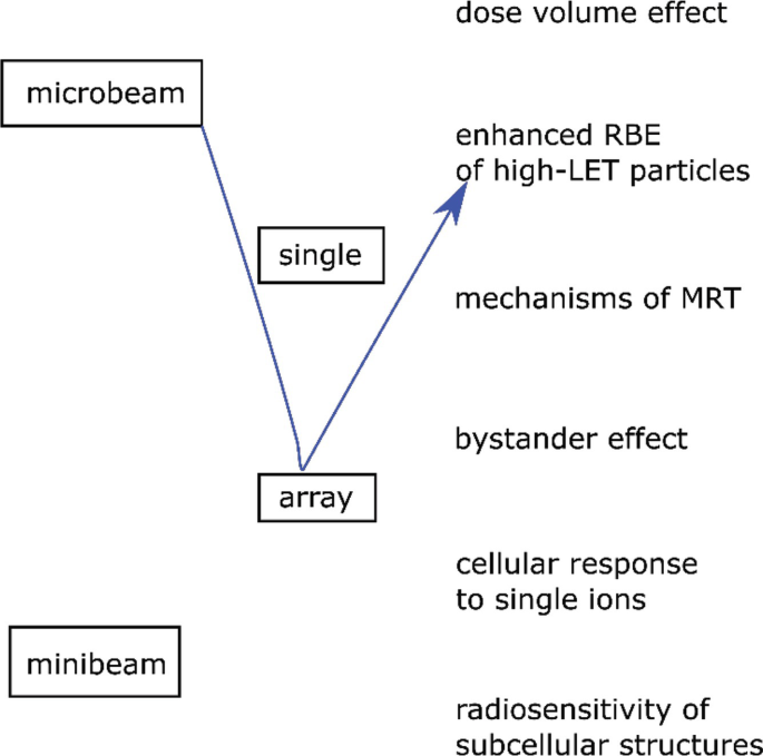
-
(a)
-
Q5.
Target theory and dose-response models

-
Use the data in the table below (A549 lung cancer cells irradiated with 220 kV X-rays) to:
-
(a)
Find the α/β-value both from a LQ-fitting and by drawing the initial slope and comparing the contributions from each term (see figure provided in Sect. 4.5 above).
-
(b)
Calculate the surviving fraction using α and β from your LQ-fitting for 5 fractions of 2 Gy (24 h apart) and compare to a single dose of 10 Gy.
-
(c)
How many fractions of 2 Gy should we give to get the same biological effect as for 1 fraction of 10 Gy?
-
(a)
Dose [Gy] | Surviving fraction | Standard error |
|---|---|---|
0 | 1 | |
0.5 | 0.88 | 0.07 |
1 | 0.64 | 0.06 |
2 | 0.41 | 0.04 |
5 | 0.07 | 0.02 |
10 | 0.0008 | 0.0003 |
4.7 Exercise Solutions
-
SQ1.
Principles of radiation dosimetry
-
SQ2.
Radiation microdosimetry
-
(a)
The lineal energy is the quotient of the total energy imparted to a volume of matter by a single energy deposition event and the mean chord length in that volume.
-
(b)
In large-size targets, the number of interactions is large and the distribution of lineal energy converge to an expected value, which is the LET.
-
(a)
-
SQ3.
From track structure to early DNA damage
-
1.
Two main characteristics differentiate these two types of MC calculation:
-
(a)
TS MC codes do not use the condensed history approach for electron transport and they discretely simulate all electron interactions (elastic and inelastic)
-
(b)
TS MC codes include electron interaction cross sections to explicitly transport the electrons down to very low energies (of the order of 10 eV), which allows to calculate the energy depositions in micrometric and nanometric volumes.
-
(a)
-
2.
Cross sections, mainly for liquid water, used by MCTS codes have uncertainties due to the lack of experimental data that could validate them. All the complexity of radiolysis and reactions of radiolytic species with biomolecules is not taken into account. DNA geometrical models require approximations. The conversion of particle interactions or reactions of radiolytic species into damage is a source of interpretation.
-
1.
-
SQ4.
Micro-beams and Minibeams
-
(a)
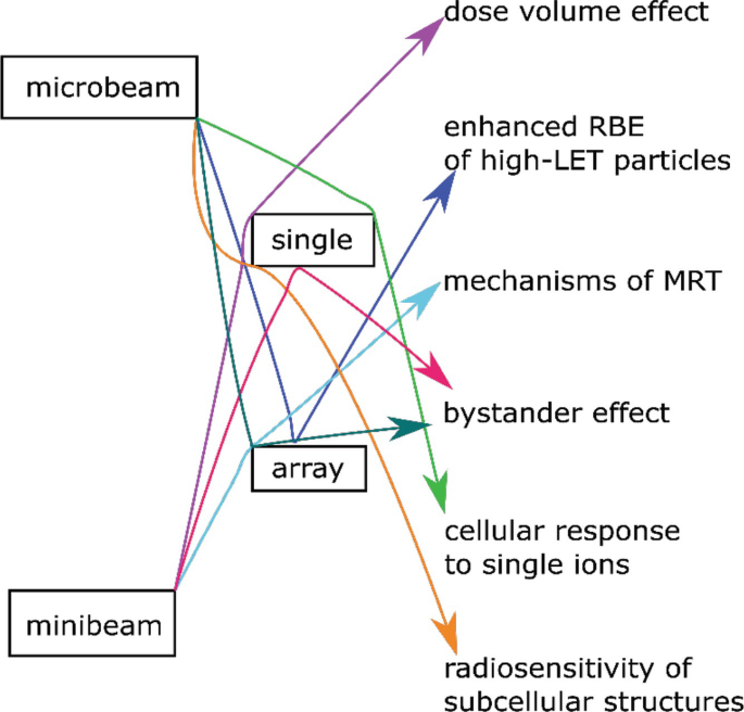

-
SQ5.
Target theory and dose-response models
-
(a)
α/β = 12
-
(b)
and 0.001
-
(c)
8
-
(a)
References
Attix FH. Introduction to radiological physics and radiation dosimetry. New York: Wiley; 1986.
Pawlicki T, Scanderbeg DJ, Starkschall G, Hendee WR. Hendee’s radiation therapy physics. 4th ed. Hoboken: Wiley; 2016.
Attix FH. Energy imparted, energy transferred and net energy transferred. Phys Med Biol. 1983;28:1385–90.
Carlsson CA, Carlsson GA. Chapter 2: Dosimetry in diagnostic radiology and computerized tomography. In: Kase KR, Bjärngard BE, Attix FH, editors. The dosimetry of ionizing radiation. San Diego: Academic Press; 1990. p. 163–257. https://doi.org/10.1016/B978-0-12-400403-0.50006-3.
Gustafsson M. Energy imparted in roentgen diagnostic procedures. Results of two surveys during the periods 1958–1960 and 1974–1976 related to technical modifications. Acta Radiol Diagn (Stockh). 1979;20:123–44.
Das A. Introduction to nuclear and particle physics. Singapore: World Scientific; 2003.
Martin BR, Shaw G. Nuclear and particle physics: an introduction. 3rd ed. Hoboken: Wiley; 2019.
Hachadorian RL, Bruza P, Jermyn M, Gladstone DJ, Pogue BW, Jarvis LA. Imaging radiation dose in breast radiotherapy by X-ray CT calibration of Cherenkov light. Nat Commun. 2020;11:2298. https://doi.org/10.1038/s41467-020-16031-z.
Allison J, Amako K, Apostolakis JEA, Araujo H, Dubois PA, Asai M, et al. Geant4 developments and applications. IEEE Trans Nucl Sci. 2006;53:270–8.
Goorley T, James M, Booth T, Brown F, Bull J, Cox LJ, et al. Initial MCNP6 release overview. Nucl Technol. 2012;180:298–315. https://doi.org/10.13182/NT11-135.
Kawrakow I, Rogers DWO. The EGSnrc code system: Monte Carlo simulation of electron and photon transport. 2010
Pelowitz DB. MCNPX user’s manual version 2.5.0. Los Alamos Natl Lab. 2005;76:473.
PENELOPE 2008 (2008: Barcelona), Francesc SG, Fernández Varea JM, Sempau Roma J. Organització de Cooperació i Desenvolupament Econòmic. PENELOPE-2008 workshop proceedings Barcelona, Spain 30 June–3 July, 2008. Paris: OECD; 2009.
ICRU. REPORT 35—Radiation dosimetry: electron beams with energies between 1 and 50 MeV | Engineering 360. ICRU; 1984.
Rossi HH, Biavati MH, Gross W. Local energy density in irradiated tissues: I. Radiobiological significance. Radiat Res. 1961;15:431. https://doi.org/10.2307/3571286.
Rossi HH, Rosenzweig W. A device for the measurement of dose as a function of specific ionization. Radiology. 1955;64:404–11. https://doi.org/10.1148/64.3.404.
Booz J, Braby L, Coyne J, Kliauga P, Lindborg L, Menzel H-G, et al. Microdosimetry. J Int Comm Radiat Units Meas. 1983;os19:36. https://doi.org/10.1093/jicru/os19.1.Report36.
Magrin G. A method to convert spectra from slab microdosimeters in therapeutic ion-beams to the spectra referring to microdosimeters of different shapes and material. Phys Med Biol. 2018;63:215021. https://doi.org/10.1088/1361-6560/aae655.
Hawkins RB. A statistical theory of cell killing by radiation of varying linear energy transfer. Radiat Res. 1994;140:366. https://doi.org/10.2307/3579114.
Kase Y, Kanai T, Matsumoto Y, Furusawa Y, Okamoto H, Asaba T, et al. Microdosimetric measurements and estimation of human cell survival for heavy-ion beams. Radiat Res. 2006;166:629–38.
Jorgensen TJ. Enhancing radiosensitivity: targeting the DNA repair pathways. Cancer Biol Ther. 2009;8:665–70. https://doi.org/10.4161/cbt.8.8.8304.
Dingfelder M, Jorjishvili IG, Gersh JA, Toburen LH. Heavy ion track structure simulations in liquid water at relativistic energies. Radiat Prot Dosimetry. 2006;122:26–7. https://doi.org/10.1093/rpd/ncl415.
Muroya Y, Plante I, Azzam EI, Meesungnoen J, Katsumura Y, Jay-Gerin J-P. High-LET ion radiolysis of water: visualization of the formation and evolution of ion tracks and relevance to the radiation-induced bystander effect. Radiat Res. 2006;165:485–91. https://doi.org/10.1667/RR3540.1.
Pimblott SM, LaVerne JA. Production of low-energy electrons by ionizing radiation. Radiat Phys Chem. 2007;76:1244–7.
Plante I, Cucinotta FA. Ionization and excitation cross sections for the interaction of HZE particles in liquid water and application to Monte Carlo simulation of radiation tracks. New J Phys. 2008;10:125020.
Michaud M, Wen A, Sanche L. Cross sections for low-energy (1–100 eV) electron elastic and inelastic scattering in amorphous ice. Radiat Res. 2003;159:3–22.
Emfietzoglou D, Kyriakou I, Garcia-Molina R, Abril I. Inelastic mean free path of low-energy electrons in condensed media: beyond the standard models. Surf Interface Anal. 2017a;49:4–10.
Boudaıffa B, Cloutier P, Hunting D, Huels MA, Sanche L. Resonant formation of DNA strand breaks by low-energy (3–20 eV) electrons. Science. 2000;287:1658–60.
Huels MA, Boudaïffa B, Cloutier P, Hunting D, Sanche L. Single, double, and multiple double strand breaks induced in DNA by 3–100 eV electrons. J Am Chem Soc. 2003;125:4467–77.
Prise KM. Critical energies for SSB and DSB induction in plasmid DNA by low-energy photons: action spectra for strand-break induction in plasmid DNA irradiated in vacuum. Int J Radiat Biol. 2000;76:881–90.
Buxton GV, Greenstock CL, Helman WP, Ross AB. Critical review of rate constants for reactions of hydrated electrons, hydrogen atoms and hydroxyl radicals (⋅OH/⋅O⋅−) in aqueous solution. J Phys Chem Ref Data. 1988;17:513–886. https://doi.org/10.1063/1.555805.
Plante I. A review of simulation codes and approaches for radiation chemistry. Phys Med Biol. 2021;66:03TR02.
Green NJB, Pilling MJ, Pimblott SM, Clifford P. Stochastic modeling of fast kinetics in a radiation track. J Phys Chem. 1990;94:251–8.
Berg HC. Random walks in biology. Princeton: Princeton University Press; 1993.
Frongillo Y, Goulet T, Fraser MJ, Cobut V, Patau JP, Jay-Gerin JP. Monte Carlo simulation of fast electron and proton tracks in liquid water-II. Nonhomogeneous chemistry. Radiat Phys Chem. 1998;51:245–54.
Tomita H, Kai M, Kusama T, Ito A. Monte Carlo simulation of physicochemical processes of liquid water radiolysis. Radiat Environ Biophys. 1997;36:105–16.
Karamitros M, Luan S, Bernal MA, Allison J, Baldacchino G, Davidkova M, et al. Diffusion-controlled reactions modeling in Geant4-DNA. J Comput Phys. 2014;274:841–82. https://doi.org/10.1016/j.jcp.2014.06.011.
Uehara S, Nikjoo H. Monte Carlo simulation of water radiolysis for low-energy charged particles. J Radiat Res (Tokyo). 2006;47:69–81. https://doi.org/10.1269/jrr.47.69.
Cadet J, Douki T, Gasparutto D, Ravanat J-L. Oxidative damage to DNA: formation, measurement and biochemical features. Mutat Res Mol Mech Mutagen. 2003;531:5–23.
Frankenberg-Schwager M. Induction, repair and biological relevance of radiation-induced DNA lesions in eukaryotic cells. Radiat Environ Biophys. 1990;29:273–92.
Boscolo D, Scifoni E, Durante M, Krämer M, Fuss MC. May oxygen depletion explain the FLASH effect? A chemical track structure analysis. Radiother Oncol. 2021;162:68–75.
Curtis SB. Lethal and potentially lethal lesions induced by radiation—a unified repair model. Radiat Res. 1986;106:252–70.
Goodhead DT. Saturable repair models of radiation action in mammalian cells. Radiat Res. 1985;104:S58–67.
Tobias CA. The repair–misrepair model in radiobiology: comparison to other models. Radiat Res. 1985;104:S77–95.
Campa A, Ballarini F, Belli M, Cherubini R, Dini V, Esposito G, et al. DNA DSB induced in human cells by charged particles and gamma rays: experimental results and theoretical approaches. Int J Radiat Biol. 2005;81:841–54.
Friedland W, Jacob P, Bernhardt P, Paretzke HG, Dingfelder M. Simulation of DNA damage after proton irradiation. Radiat Res. 2003;159:401–10.
Nikjoo H, O’Neill P, Wilson WE, Goodhead DT. Computational approach for determining the spectrum of DNA damage induced by ionizing radiation. Radiat Res. 2001;156:577–83.
Meylan S, Incerti S, Karamitros M, Tang N, Bueno M, Clairand I, et al. Simulation of early DNA damage after the irradiation of a fibroblast cell nucleus using Geant4-DNA. Sci Rep. 2017;7:1–15.
Rogakou EP, Pilch DR, Orr AH, Ivanova VS, Bonner WM. DNA double-stranded breaks induce histone H2AX phosphorylation on serine 139. J Biol Chem. 1998;273:5858–68.
Lorat Y, Brunner CU, Schanz S, Jakob B, Taucher-Scholz G, Rübe CE. Nanoscale analysis of clustered DNA damage after high-LET irradiation by quantitative electron microscopy—the heavy burden to repair. DNA Repair. 2015;28:93–106.
Barbieri S, Babini G, Morini J, Friedland W, Buonanno M, Grilj V, et al. Predicting DNA damage foci and their experimental readout with 2D microscopy: a unified approach applied to photon and neutron exposures. Sci Rep. 2019;9:1–17.
Gonon G, Villagrasa C, Voisin P, Meylan S, Bueno M, Benadjaoud MA, et al. From energy deposition of ionizing radiation to cell damage signaling: benchmarking simulations by measured yields of initial DNA damage after ion microbeam irradiation. Radiat Res. 2019;191:566–84.
Nikjoo H, Uehara S, Emfietzoglou D, Cucinotta FA. Track-structure codes in radiation research. Radiat Meas. 2006;41:1052–74.
Dingfelder M. Track structure: time evolution from physics to chemistry. Radiat Prot Dosimetry. 2006;122:16–21.
Kyriakou I, Sakata D, Tran HN, Perrot Y, Shin W-G, Lampe N, et al. Review of the geant4-dna simulation toolkit for radiobiological applications at the cellular and DNA level. Cancers. 2022;14:35.
Hayashi H, Watanabe N, Udagawa Y, Kao C-C. The complete optical spectrum of liquid water measured by inelastic X-ray scattering. Proc Natl Acad Sci. 2000;97:6264–6.
Heller JM Jr, Hamm RN, Birkhoff RD, Painter LR. Collective oscillation in liquid water. J Chem Phys. 1974;60:3483–6.
Villagrasa C, Francis Z, Incerti S. Physical models implemented in the GEANT4-DNA extension of the GEANT-4 toolkit for calculating initial radiation damage at the molecular level. Radiat Prot Dosimetry. 2011;143:214–8.
Champion C. Theoretical cross sections for electron collisions in water: structure of electron tracks. Phys Med Biol. 2003;48:2147.
Emfietzoglou D, Papamichael G, Nikjoo H. Monte Carlo electron track structure calculations in liquid water using a new model dielectric response function. Radiat Res. 2017b;188:355–68.
Garcia-Molina R, Abril I, Kyriakou I, Emfietzoglou D. Inelastic scattering and energy loss of swift electron beams in biologically relevant materials. Surf Interface Anal. 2017;49:11–7.
Emfietzoglou D, Kyriakou I, Abril I, Garcia-Molina R, Nikjoo H. Inelastic scattering of low-energy electrons in liquid water computed from optical-data models of the Bethe surface. Int J Radiat Biol. 2012;88:22–8.
Villagrasa C, Bordage M-C, Bueno M, Bug M, Chiriotti S, Gargioni E, et al. Assessing the contribution of cross-sections to the uncertainty of Monte Carlo calculations in micro-and nanodosimetry. Radiat Prot Dosimetry. 2019;183:11–6.
Lampe N, Karamitros M, Breton V, Brown JM, Kyriakou I, Sakata D, et al. Mechanistic DNA damage simulations in Geant4-DNA part 1: a parameter study in a simplified geometry. Phys Med. 2018;48:135–45.
de Vera P, Abril I, Garcia-Molina R. Excitation and ionisation cross-sections in condensed-phase biomaterials by electrons down to very low energy: application to liquid water and genetic building blocks. Phys Chem Chem Phys. 2021;23:5079–95.
Nguyen-Truong HT. Low-energy electron inelastic mean free paths for liquid water. J Phys Condens Matter. 2018;30:155101.
Quinto MA, Monti JM, Week PF, Fojón OA, Hanssen J, Rivarola RD, et al. TILDA-V: a full-differential code for proton tracking in biological matter. J Phys Conf Ser. 2015;635:032063.
Verkhovtsev A, Traore A, Muñoz A, Blanco F, García G. Modeling secondary particle tracks generated by intermediate-and low-energy protons in water with the low-energy particle track simulation code. Radiat Phys Chem. 2017;130:371–8.
Signorell R. Electron scattering in liquid water and amorphous ice: a striking resemblance. Phys Rev Lett. 2020;124:205501.
Zein SA, Bordage M-C, Francis Z, Macetti G, Genoni A, Dal Cappello C, et al. Electron transport in DNA bases: an extension of the Geant4-DNA Monte Carlo toolkit. Nucl Instrum Methods Phys Res Sect B Beam Interact Mater At. 2021;488:70–82.
Uehara S, Nikjoo H, Goodhead DT. Cross-sections for water vapour for the Monte Carlo electron track structure code from 10 eV to the MeV region. Phys Med Biol. 1993;38:1841.
Sempau J, Fernández-Varea JM, Acosta E, Salvat F. Experimental benchmarks of the Monte Carlo code PENELOPE. Nucl Instrum Methods Phys Res Sect B Beam Interact Mater At. 2003;207:107–23.
Shin W, Bordage M, Emfietzoglou D, Kyriakou I, Sakata D, Min C, et al. Development of a new Geant4-DNA electron elastic scattering model for liquid-phase water using the ELSEPA code. J Appl Phys. 2018;124:224901.
Charlton DE, Nikjoo H, Humm JL. Calculation of initial yields of single-and double-strand breaks in cell nuclei from electrons, protons and alpha particles. Int J Radiat Biol. 1989;56:1–19.
Nikjoo H, Goodhead DT, Charlton DE, Paretzke HG. Energy deposition in small cylindrical targets by ultrasoft X-rays. Phys Med Biol. 1989;34:691.
Pomplun E. A new DNA target model for track structure calculations and its first application to I-125 Auger electrons. Int J Radiat Biol. 1991;59:625–42.
Meylan S, Vimont U, Incerti S, Clairand I, Villagrasa C. Geant4-DNA simulations using complex DNA geometries generated by the DnaFabric tool. Comput Phys Commun. 2016;204:159–69.
Tang N, Bueno M, Meylan S, Incerti S, Tran HN, Vaurijoux A, et al. Influence of chromatin compaction on simulated early radiation-induced DNA damage using Geant4-DNA. Med Phys. 2019;46:1501–11.
Friedland W, Dingfelder M, Kundrát P, Jacob P. Track structures, DNA targets and radiation effects in the biophysical Monte Carlo simulation code PARTRAC. Mutat Res Mol Mech Mutagen. 2011a;711:28–40.
Lobachevsky PN, Martin RF. DNA strand breakage by 125I-decay in a synthetic oligodeoxynucleotide: quantitative analysis of fragment distribution. Acta Oncol. 1996;35:809–15.
Friedland W, Jacob P, Kundrat P. Mechanistic simulation of radiation damage to DNA and its repair: on the track towards systems radiation biology modelling. Radiat Prot Dosimetry. 2011b;143:542–8.
Friedland W, Schmitt E, Kundrát P, Dingfelder M, Baiocco G, Barbieri S, et al. Comprehensive track-structure based evaluation of DNA damage by light ions from radiotherapy-relevant energies down to stopping. Sci Rep. 2017;7:1–15.
Nikjoo H, Martin RF, Charlton DE, Terrissol M, Kandaiya S, Lobachevsky P. Modelling of Auger-induced DNA damage by incorporated125I. Acta Oncol. 1996;35:849–56.
Schuemann J, McNamara AL, Warmenhoven JW, Henthorn NT, Kirkby KJ, Merchant MJ, et al. A new standard DNA damage (SDD) data format. Radiat Res. 2019;191:76–92.
Zirkle RE, Bloom W. Irradiation of parts of individual cells. Science. 1953;117:487–93.
Withers HR, Thames HD. Dose fractionation and volume effects in normal tissues and tumors. Am J Clin Oncol. 1988;11:313–29.
Folkard B, Vojnovic KJ, Hollis M. A charged-particle microbeam: II. A single-particle micro-collimation and detection system. Int J Radiat Biol. 1997a;72:387–95. https://doi.org/10.1080/095530097143167.
Randers-Pehrson G, Geard CR, Johnson G, Elliston CD, Brenner DJ. The Columbia University single-ion microbeam. Radiat Res. 2001;156:210–4.
Brenner DJ, Miller RC, Huang Y, Hall EJ. The biological effectiveness of radon-progeny alpha particles. III. Quality factors. Radiat Res. 1995;142:61–9.
Cole A. Mechanisms of cell injury. In: Radiation biology in cancer research. New York: Raven Press; 1980. p. 33–58.
Siebenwirth C, Greubel C, Drexler GA, Reindl J, Walsh DWM, Schwarz B, et al. Local inhibition of rRNA transcription without nucleolar segregation after targeted ion irradiation of the nucleolus. J Cell Sci. 2019;132:jcs.232181. https://doi.org/10.1242/jcs.232181.
Walsh DW, Siebenwirth C, Greubel C, Ilicic K, Reindl J, Girst S, et al. Live cell imaging of mitochondria following targeted irradiation in situ reveals rapid and highly localized loss of membrane potential. Sci Rep. 2017;7:1–11.
Deshpande A, Goodwin EH, Bailey SM, Marrone BL, Lehnert BT. Alpha-particle-induced sister chromatid exchange in normal human lung fibroblasts: evidence for an extranuclear target. Radiat Res. 1996;145:260–7.
Dollinger G. Life cell micro-irradiation. Nucl Phys News. 2010;20:27–32. https://doi.org/10.1080/10619127.2010.506125.
Hauptner A, Cremer T, Deutsch M, Dietzel S, Drexler GA, Greubel C, et al. Irradiation of living cells with single ions at the ion microprobe SNAKE. ACTA Phys Pol Ser A. 2006;109:273.
Voss KO, Fournier C, Taucher-Scholz G, Voss KO, Fournier C, Taucher-Scholz G. Heavy ion microprobes: a unique tool for bystander research and other radiobiological applications. New J Phys. 2008;10:075011. https://doi.org/10.1088/1367-2630/10/7/075011.
Kobayashi K, Usami N, Maezawa H, Hayashi T, Hieda K, Takakura K. Synchrotron X-ray microbeam irradiation system for radiobiology. J Biomed Nanotechnol. 2006;2:116–9.
Folkard M, Vojnovic B, Schettino G, Forsberg M, Bowey G, Prise KM, et al. Two approaches for irradiating cells individually: a charged-particle microbeam and a soft X-ray microprobe. Nucl Instrum Methods Phys Res Sect B Beam Interact Mater At. 1997b;130:270–4.
Greubel C, Ilicic K, Rösch T, Reindl J, Siebenwirth C, Moser M, et al. Low LET proton microbeam to understand high-LET RBE by shaping spatial dose distribution. Nucl Instrum Methods Phys Res Sect B Beam Interact Mater At. 2017;404:155–61. https://doi.org/10.1016/j.nimb.2016.11.032.
Schmid TE, Greubel C, Hable V, Zlobinskaya O, Michalski D, Girst S, et al. Low LET protons focused to submicrometer shows enhanced radiobiological effectiveness. Phys Med Biol. 2012;57:5889–907. https://doi.org/10.1088/0031-9155/57/19/5889.
Tao Y, Tan HQ, Mi Z, Chen C-B, Lam VYM, Osipowicz T, et al. The radiobiology beam line facility at the Centre for Ion Beam Applications, National University of Singapore. Nucl Instrum Methods Phys Res Sect B Beam Interact Matter At. 2019;456:26–31. https://doi.org/10.1016/j.nimb.2019.06.038.
Miller RC, Randers-Pehrson G, Geard CR, Hall EJ, Brenner DJ. The oncogenic transforming potential of the passage of single α particles through mammalian cell nuclei. Proc Natl Acad Sci. 1999;96:19–22.
Shao C, Folkard M, Michael BD, Prise KM. Bystander signaling between glioma cells and fibroblasts targeted with counted particles. Int J Cancer. 2005;116:45–51.
Sawant SG, Randers-Pehrson G, Metting NF, Hall EJ. Adaptive response and the bystander effect induced by radiation in C3H 10 T1/2 cells in culture. Radiat Res. 2001;156:177–80.
Yokoya A, Usami N. Targeting specific sites in biological systems with synchrotron X-ray micro-beams for radiobiological studies at the photon factory. Quantum Beam Sci. 2020;4:2. https://doi.org/10.3390/qubs4010002.
Hable V, Drexler GA, Brüning T, Burgdorf C, Greubel C, Derer A, et al. Recruitment kinetics of DNA repair proteins Mdc1 and Rad52 but not 53BP1 depend on damage complexity. PLoS One. 2012;7:e41943. https://doi.org/10.1371/journal.pone.0041943.
Buchfellner A, Yurlova L, Nüske S, Scholz AM, Bogner J, Ruf B, et al. A new nanobody-based biosensor to study endogenous PARP1 in vitro and in live human cells. PLoS One. 2016;11:e0151041. https://doi.org/10.1371/journal.pone.0151041.
Girst S, Hable V, Drexler GA, Greubel C, Siebenwirth C, Haum M, et al. Subdiffusion supports joining of correct ends during repair of DNA double-strand breaks. Sci Rep. 2013;3:1–6.
Friedland W, Kundrát P, Schmitt E, Becker J, Ilicic K, Greubel C, et al. Modeling studies on dicentrics induction after sub-micrometer focused ion beam grid irradiation. Radiat Prot Dosimetry. 2019;183:40–4.
Friedrich T, Ilicic K, Greubel C, Girst S, Reindl J, Sammer M, et al. DNA damage interactions on both nanometer and micrometer scale determine overall cellular damage. Sci Rep. 2018;8:1–10.
Schmid TE, Friedland W, Greubel C, Girst S, Reindl J, Siebenwirth C, et al. Sub-micrometer 20 MeV protons or 45 MeV lithium spot irradiation enhances yields of dicentric chromosomes due to clustering of DNA double-strand breaks. Mutat Res Toxicol Environ Mutagen. 2015;793:30–40.
Dertinger H, Jung H. Molecular radiation biology: the action of ionizing radiation on elementary biological objects. New York: Springer; 1970.
Rauth AM, Simpson JA. The energy loss of electrons in solids. Radiat Res. 1964;22:643–61. https://doi.org/10.2307/3571545.
McMahon SJ. The linear quadratic model: usage, interpretation and challenges. Phys Med Biol. 2018;64:01TR01. https://doi.org/10.1088/1361-6560/aaf26a.
Kellerer AM, Rossi HH. RBE and the primary mechanism of radiation action. Radiat Res. 1971;47:15. https://doi.org/10.2307/3573285.
Chadwick KH, Leenhouts HP. A molecular theory of cell survival. Phys Med Biol. 1973;18:78–87. https://doi.org/10.1088/0031-9155/18/1/007.
Bodgi L, Foray N. The nucleo-shuttling of the ATM protein as a basis for a novel theory of radiation response: resolution of the linear-quadratic model. Int J Radiat Biol. 2016;92:117–31. https://doi.org/10.3109/09553002.2016.1135260.
Marples B, Joiner MC. The response of Chinese hamster V79 cells to low radiation doses: evidence of enhanced sensitivity of the whole cell population. Radiat Res. 1993;133:41–51.
Joiner MC, Johns H. Renal damage in the mouse: the response to very small doses per fraction. Radiat Res. 1988;114:385–98.
Garcia LM, Leblanc J, Wilkins D, Raaphorst GP. Fitting the linear–quadratic model to detailed data sets for different dose ranges. Phys Med Biol. 2006;51:2813.
Kirkpatrick JP, Meyer JJ, Marks LB. The linear-quadratic model is inappropriate to model high dose per fraction effects in radiosurgery. Semin Radiat Oncol. 2008;18:240–3. https://doi.org/10.1016/j.semradonc.2008.04.005.
Guerrero M, Li XA. Extending the linear–quadratic model for large fraction doses pertinent to stereotactic radiotherapy. Phys Med Biol. 2004;49:4825.
Hall EJ, Giaccia AJ. Radiobiology for the radiologist. Philadelphia: Lippincott Williams & Wilkins; 2012.
Stapleton GE, Billen D, Hollaender A. Recovery of X-irradiated bacteria at suboptimal incubation temperatures. J Cell Comp Physiol. 1953;41:345–57.
Phillips RA, Tolmach LJ. Repair of potentially lethal damage in X-irradiated HeLa cells. Radiat Res. 1966;29:413–32.
Shipley WU, Stanley JA, Courtenay VD, Field SB. Repair of radiation damage in Lewis lung carcinoma cells following in situ treatment with fast neutrons and gamma-rays. Cancer Res. 1975;35:932–8.
Weichselbaum RR, Little JB. Repair of potentially lethal X-ray damage and possible applications to clinical radiotherapy. Int J Radiat Oncol Biol Phys. 1983;9:91–6.
Lorat Y, Timm S, Jakob B, Taucher-Scholz G, Rübe CE. Clustered double-strand breaks in heterochromatin perturb DNA repair after high linear energy transfer irradiation. Radiother Oncol. 2016;121:154–61.
Puck TT, Marcus PI. Action of X-rays on mammalian cells. J Exp Med. 1956;103:653–66.
Elkind MM, Sutton H. X-ray damage and recovery in mammalian cells in culture. Nature. 1959;184:1293–5.
Elkind MM, Sutton-Gilbert H, Moses WB, Alescio T, Swain R. Radiation response of mammalian cells grown in culture: V. Temperature dependence of the repair of X-ray damage in surviving cells (aerobic and hypoxic). Radiat Res. 1965;25:359–76.
Elkind MM, Sutton H. Radiation response of mammalian cells grown in culture: I. Repair of X-ray damage in surviving Chinese hamster cells. Radiat Res. 1960;13:556–93.
Steel GG. The ESTRO Breur lecture cellular sensitivity to low dose rate irradiation focuses the problem of tumour radioresistance. Radiother Oncol. 1991;20:71–83.
Furre T. Inverse dose rate effect due to pre-mitotic accumulation during continuous low dose rate irradiation of cervix carcinoma cells. Int J Radiat Biol. 1999;75:699–707.
Furre T, Eggen Furre I, Koritzinsky M, Åmellem Ø, Pettersen EO. Lack of inverse dose rate effect and binding of the retinoblastoma gene product in the nucleus of human cancer T-47D cells arrested in G2 by ionizing radiation. Int J Radiat Biol. 2003;79:413–22.
Stewart FA, Soranson JA, Alpen EL, Williams MV, Denekamp J. Radiation-induced renal damage: the effects of hyperfractionation. Radiat Res. 1984;98:407–20.
Joiner MC, Bentzen SM. Fractionation: the linear-quadratic approach. In: Basic clinical radiobiology. 4th ed. Boca Raton: CRC Press; 2009.
Fowler JF. The radiobiology of prostate cancer including new aspects of fractionated radiotherapy. Acta Oncol Stockh Swed. 2005;44:265–76. https://doi.org/10.1080/02841860410002824.
Fowler JF. La Ronde—radiation sciences and medical radiology. Radiother Oncol. 1983;1:1–22.
United Nations Scientific Committee on the Effects of Atomic Radiation. Sources and effects of ionizing radiation, United Nations scientific committee on the effects of atomic radiation (UNSCEAR) 1993 report: report to the general assembly, with scientific annexes. New York: United Nations; 1993.
Nias AHW. An introduction to radiobiology. New York: Wiley; 1998.
ICRP. ICRP Publication 60: 1990 Recommendations of the International Commission on Radiological Protection. Amsterdam: Elsevier; 1991.
National Research Council (U.S.). Health effects of exposure to low levels of ionizing radiation: BEIR V. Washington, DC: National Academy Press; 1990.
Calabrese EJ. The road to linearity: why linearity at low doses became the basis for carcinogen risk assessment. Arch Toxicol. 2009;83:203–25.
Feinendegen LE. Conference summary. Health Phys. 2020;118:322–6. https://doi.org/10.1097/HP.0000000000001207.
Rattan SIS, Kyriazis M, editors. The science of hormesis in health and longevity. London: Academic Press; 2019.
Further Reading
Principles of Radiation Dosimetry
Radiation Microdosimetry
Lindborg L, Waker A. Microdosimetry: experimental methods and applications. Boca Raton: CRC Press; 2017.
From Track Structure to Early DNA Damage
Micro-beams and Minibeams
Radiation Protection Dosimetry, Section: Micro-beams and biological applications. https://academic.oup.com/rpd/search-results?f_TocHeadingTitle=Micro-beams+and+biological+applications.
Target Theory and Dose Response Models
Chapman JD, Nahum AE. Radiotherapy treatment planning—linear-quadratic radiobiology. Boca Raton: CRC Press Inc; 2015.
Author information
Authors and Affiliations
Corresponding author
Editor information
Editors and Affiliations
Rights and permissions
Open Access This chapter is licensed under the terms of the Creative Commons Attribution 4.0 International License (http://creativecommons.org/licenses/by/4.0/), which permits use, sharing, adaptation, distribution and reproduction in any medium or format, as long as you give appropriate credit to the original author(s) and the source, provide a link to the Creative Commons license and indicate if changes were made.
The images or other third party material in this chapter are included in the chapter's Creative Commons license, unless indicated otherwise in a credit line to the material. If material is not included in the chapter's Creative Commons license and your intended use is not permitted by statutory regulation or exceeds the permitted use, you will need to obtain permission directly from the copyright holder.
Copyright information
© 2023 The Author(s)
About this chapter

Cite this chapter
Schettino, G. et al. (2023). Mechanistic, Modeling, and Dosimetric Radiation Biology. In: Baatout, S. (eds) Radiobiology Textbook. Springer, Cham. https://doi.org/10.1007/978-3-031-18810-7_4
Download citation
DOI: https://doi.org/10.1007/978-3-031-18810-7_4
Published:
Publisher Name: Springer, Cham
Print ISBN: 978-3-031-18809-1
Online ISBN: 978-3-031-18810-7
eBook Packages: MedicineMedicine (R0)