
Abstract
In applied computations the need arises to define, for example, a discrete field with assigned curl or to represent a div-free field in a given discrete space. In the low degree case this need is often fulfilled by employing tree and co-tree techniques. The definition of tree and co-tree is thus revisited here in the frame of high order Whitney element reconstructions. We consider the case of fields that are reconstructed in a contractible polyhedral domain \(\varOmega \in \mathbb R^3\), with connected boundary ∂Ω, starting from their weights over suitable “small simplices” in a simplicial mesh \({\mathcal M}\) of the domain \(\bar \varOmega \).
You have full access to this open access chapter, Download conference paper PDF
1 Introduction
We aim at determining in a constructive way, for the high order case, the finite element solutions of grad ϕ = E, curl A = B, div D = ρ, namely, of the equations linking the electric field E, the magnetic induction B, and the electric charge density ρ, to their potentials ϕ, A and D, respectively. Stating the necessary and sufficient conditions for assuring that a function defined in a bounded set \(\varOmega \subset {\mathbb R}^3 \) is the gradient of a scalar potential, the curl of a vector potential or the divergence of a vector field is one of the most classical problem of vector analysis (see for example [4, 8, 10]). We aim at providing an explicit and efficient procedure to construct a finite element solution. For example, div-free fields, W, are implicitly characterized in terms of a vector w of degrees of freedom of W by the algebraic constraint D w = 0, with D the matrix of the div operator between finite elements spaces. The same fields, in the case of a domain with connected boundary, are explicitly defined by w = R a, with no constraint on a, where R is the matrix of the curl operator between finite elements spaces and a collects the degrees of freedom of the vector potentials A. Similarly, one can wish to compute a vector potential a such that R a = b, for a given field b verifying D b = 0. As explained in [6], these bases can be constructed by the help of “trees” and “co-trees”, which are at the core of this contribution. The case r = 0 is largely treated in the literature for different types of topological domains (see for example [2]). In these pages, we develop the tree and co-tree approaches for r > 0 when fields in the high order Whitney spaces are represented on the basis of their weights on small simplices [7, 9, 12]. With this choice of degrees of freedom, the tree and co-tree concepts extend from r = 0 to r > 0 straightforwardly.
2 Basic Concepts
Let \(\varOmega \subset {\mathbb R}^3\) be a bounded polyhedral domain with Lipschitz boundary ∂Ω and \({\mathcal M}\) a simplicial mesh of \(\bar \varOmega \). We denote by |A| the cardinality of the set A. For 0 ≤ k ≤ 3, let Δ k(T) (resp. \(\varDelta _k({\mathcal M})\)) be the set of k-simplices of a mesh tetrahedron T (resp. of the mesh \({\mathcal M}\)). Note that \(\varDelta _k({\mathcal M}) = \cup _{T \in {\mathcal M}} \varDelta _k(T)\). If \(\varDelta _0({\mathcal M}) = \{ {\mathbf {v}}_i\}_{i}\), with i = 1, …, N v, being \(N_v = |\varDelta _0({\mathcal M})|\), then each k-simplex \(S \in \varDelta _k({\mathcal M})\) has associated an increasing map m S : {0, …, k} → {1, …, N v}. This map induces an (inner) orientation on S (i.e., a way to run along S if k = 1, through S if k = 2, in S if k = 3).
If we assign to each \(S \in \varDelta _k({\mathcal M}) \) a real number c S we can define the k-chain \(c = \sum _{S \in \varDelta _0({\mathcal M}) } {c_S} \, S\), i.e. a formal weighted sum of k-simplices S in \({\mathcal M}\). One can add k-chains, namely \((c + \tilde c) = \sum _S ({c_S + \tilde c_S})\,S\), and multiply a k-chain by a scalar p, namely p c =∑S(p c S) S. The set of all k-chains in \({\mathcal M}\), here denoted \({\mathcal C}_k({\mathcal M})\), is a vector space, in one-to-one correspondence with the set of real vectors \({c} = ({ c}_S)_{S \in \varDelta _k({\mathcal M})}\). Each k-simplex \(S \in \varDelta _k({\mathcal M}) \), can be associated with the elementary k-chain c with entries c S = 1 and \({ c}_{\tilde S} = 0\) for \(\tilde S \neq S\). In the following we will use the same symbol S to denote the oriented k-simplex and the associated elementary k-chain.
The boundary operator ∂ takes a k-simplex S and returns the sum of all its (k − 1)-faces f with coefficient 1 or − 1 depending of whether the orientation of the (k − 1)-face f matches or not with the orientation induced by that of the simplex S on f. Since the boundary operator is a linear mapping from \({\mathcal C}_k({\mathcal M})\) to \({\mathcal C}_{k-1}({\mathcal M})\), it can be represented by a matrix ∂ of dimension \(|\varDelta _{k-1}({\mathcal M}) | \times |\varDelta _k({\mathcal M}) |\), which is rather sparse, gathering the coefficients 0, − 1, or + 1. Note that in three dimensions, there are three nontrivial boundary operators acting, respectively, on edges, triangles and tetrahedra: ∂ 1 represented by the matrix G ⊤, ∂ 2 represented by R ⊤, and ∂ 3 represented by D ⊤. To fully specify ∂, we need to specify the boundary of each simplex S. By definition, we have
for any \(e \in \varDelta _1({\mathcal M})\), any \(f \in \varDelta _2({\mathcal M})\) and any \(T \in \varDelta _3({\mathcal M})\). For e = [v 0, v 1], f = [v 0, v 1, v 2] and T = [v 0, v 1, v 2, v 3], we have, respectively,
The subscript is removed when there is no ambiguity, since the operator needed for a particular operation is indicated from the type of the operand (e.g., ∂ 3 when ∂ applies to tetrahedra). The notion of boundary can be extended to k-chains by linearity, \(\partial c = \partial (\sum _{S \in \varDelta _k({\mathcal M}) } {\mathbf {c}}_S \, S) = \sum _{S \in \varDelta _k({\mathcal M}) } {\mathbf {c}}_S\, \partial S \).
We say that a k-chain c is closed if ∂ k c = 0. Non-trivial closed k-chains are called k-cycles and constitute the subspace \(Z_k({\mathcal M}) = \mathrm {ker}(\partial _k; \mathcal C_k({\mathcal M}))\). A k-chain c is a boundary if it exists a (k + 1)-chain γ such that c = ∂ k+1 γ. The k-boundaries constitute the subspace \(B_{k}({\mathcal M}) = \partial _{k+1} \mathcal C_{k+1}({\mathcal M})\). From the property ∂∂ = 0, we know that boundaries are cycles but not all cycles are boundaries, and we have \(B_k({\mathcal M}) \subset Z_k({\mathcal M})\). The quotient space \({\mathcal H}_k({\mathcal M}) = [Z_k({\mathcal M})/B_k({\mathcal M})]\) is the homology spaces of order k of the mesh \({\mathcal M}\), and the Betti’s number \(b_k ={ \mathrm {rank}}\,[{\mathcal H}_k({\mathcal M})]\). The presence of curl-free fields (resp. div-free fields) that are not the gradient of a scalar field (resp. the curl of a vector field) is indicated from the fact that b 1≠0 (resp. b 2 ≠ 0). We recall that Betti’s numbers are topological invariants (i.e., they depend on the domain Ω up to a homeomorphism) and do not depend on the mesh \({\mathcal M}\) on \(\bar \varOmega \) that is used to compute them (see [14] and an application in [13]).
For the high order case, we need to introduce some concepts of relative homology. Let \(\mathcal K_k({\mathcal M})\) be subspaces of \(\mathcal C_k({\mathcal M})\) with \(\partial _k \mathcal K_k({\mathcal M}) \subset \mathcal K_{k-1}({\mathcal M})\). We thus say that \(c \in {\mathcal C}_k({\mathcal M})\) is closed [modulo \(\mathcal K_k({\mathcal M})\)] if \(\partial c \in \mathcal K_k({\mathcal M})\). A (k − 1)-chain c bounds [modulo \(\mathcal K_k({\mathcal M})\)] if there exists a k-chain γ such that \(c - \partial \gamma \in \mathcal K_{k-1}(\mathcal M)\). We thus talk about relative homology groups.
A k-cochain w (over the mesh \({\mathcal M}\)) is a linear mapping from \({\mathcal C}_k({\mathcal M})\) to \(\mathbb {R}\). They are discrete analogues to differential forms. For k > 0, the exterior derivative of the (k − 1)-form w is the k-form dw such that ∫sdw =∫∂s w for all \(s \in \mathcal {C}_{k} ({\mathcal M}).\, \) With this simple equation relating the evaluation of dw on a simplex s to the evaluation of w on the boundary of this simplex, the exterior derivative is readily defined. We can naturally extend the notion of evaluation of a differential form w on an arbitrary chain by linearity: \( \int _{\sum _i {\mathbf {c}}_i s_i} w = \sum _i {\mathbf {c}}_i \int _{s_i} w.\) Thus
The operator d is the dual of the boundary operator ∂. As a corollary of the boundary operator property ∂∂ = 0, we have that dd = 0. Since we used arrays of dimension \(|\varDelta _k({\mathcal M})|\) to represent a k-cochain, the operator d can be represented by a matrix d of dimension \(|\varDelta _k({\mathcal M})|\times |\varDelta _{k-1}({\mathcal M})|\), 1 ≤ k ≤ 3. Again, we have one matrix for the exterior derivative operator for each simplex dimension. When a metric is introduced on the ambient affine space, the exterior derivative operator d stands for grad, curl, div, according to the value of k from 1 to 3, and it is represented by, respectively, G, R, D, the connectivity matrices of the mesh \({\mathcal M}\).
3 Small Simplices, Weights and Potentials
We introduce the multi-index α = (α 0, …, α s) of s + 1 integers α i ≥ 0 and weight \(|\boldsymbol \alpha |=\sum _{i=1}^{s} \alpha _i\). The set of multi-indices α with s + 1 components and weight r is denoted \(\mathcal I(s+1, r)\). We denote by v i the (Cartesian) coordinates of the node n i in \(\mathbb R^3\). Given a multi-index \(\boldsymbol \alpha \in \mathcal I (4,r)\), and a k-subsimplex S of T, the small simplex {α, S} is the k-simplex that belongs to the small tetrahedron with barycenter at the point of coordinates \(\sum _{i=0}^3 [ (\frac {1}{4}+ \alpha _i){\mathbf {v}}_{{\sigma ^0_T(i)}}]/(r+1)\), which is parallel and 1∕(r + 1)-homothetic to the (big) sub-simplex S of T. The notation {α, S} was first defined in [7]. The set of small tetrahedra of order r + 1 > 1 can be visualized starting from the principal lattice L r+1(T) in the simplex \(T=\{n_{\sigma ^0_T(0)}\, n_{\sigma ^0_T(1)}\,n_{\sigma ^0_T(2)}\,n_{\sigma ^0_T(3)}\}\) defined as
and connecting its points by edges parallel to those of T. (See, e.g., Fig. 1.)

From the principal lattice of degree r + 1 = 3 in a tetrahedron T, we define a decomposition of T into 10 small tetrahedra, 4 octahedra O and 1 reversed tetrahedron. Each face on ∂T is decomposed into 6 small faces and 3 reversed triangles, in solid red line (Left)
We denote by Λ k(Ω) the space of all smooth differential k-forms on Ω. The completion of Λ k(Ω) in the corresponding norm defines the Hilbert space L 2 Λ k(Ω). Let \( \mathcal P^-_{r+1} \varLambda ^k(T)\) be the space of so-called trimmed polynomial k-forms of degree r + 1 on T, with r ≥ 0, (as in [9]), and we define
where HΛ k(Ω) = {ω ∈ Λ k(Ω) : dω ∈ Λ k(Ω)} is a Hilbert space (see [5]).
Definition 1
The weights of a polynomial k-form \(u \in \mathcal P^-_{r+1} \varLambda ^k(T)\), with 0 ≤ k ≤ 3 and r ≥ 0, are the scalar quantities
on the small simplices {α, S} with \(\boldsymbol \alpha \in \mathcal I (4,r)\) and S ∈ Δ k(T).
We now list some remarkable properties of the small simplices which are useful in the tree construction.
Property 1
The weights (1) of a Whitney k-form \(u \in \mathcal P_{r+1}^- \varLambda ^k(T)\) on all the small simplex {α, S} of T are unisolvent, as stated in [9, Proposition 3.14]. The small simplices can thus support the degrees of freedom for fields \(u \in \mathcal P^-_{r+1} \varLambda ^k(T)\), with 0 ≤ k ≤ 3 and r ≥ 0. Since the result on unisolvence holds true also by replacing T with F ∈ Δ n−1(T) then \(\mbox{Tr}_F u \in {\mathcal P}_{r+1}^- \varLambda ^k(F)\) is uniquely determined by the weights on small simplices in F. It thus follows that a locally defined u, with \(u_{|T} \in \mathcal P_{r+1}^- \varLambda ^k(T)\) and single-valued weights, is in HΛ k(Ω). We thus can use the weights on the small simplices {α, S} as degrees of freedom for the fields in the finite element space \(\mathcal P_{r+1}^- \varLambda ^k({\mathcal M})\) being aware that their number is greater than the dimension of the space.
Property 2
The weights given in Definition 1 have a meaning as cochains and this relates directly the matrix describing the exterior derivative with the matrix of the boundary operator. The key point is the Stokes’ theorem ∫Cdu =∫∂C u , where u is a (k − 1)-form and C a k-chain. More precisely, if \(u \in \mathcal P_{r+1}^- \varLambda ^k({\mathcal M})\) then \(z = \mathrm {d} u \in \mathcal P_{r+1}^- \varLambda ^{k+1}({\mathcal M})\) and
being B the boundary matrix with as many rows as small simplices of dimension k and as many columns as small simplices of dimension k − 1. The small simplices {α, S} inherit the orientation of the simplex S so the coefficient B {α,S},{β,F} is equal to the coefficient B S,F of the boundary of the simplex S if β = α. This is straightforward if \( \mathop {\mbox{dim}}(F)>0\) and when \( \mathop {\mbox{dim}}(F)=0\), providing that small nodes in T are given in the notation {α, n} according to their position in the small simplices when fragmented (see Fig. 1 in [1]).
Property 3
The generated \((\mbox{ }^{r+2}_{\ \ 2})\) small faces on each face F of T, pave F together with the \((\mbox{ }^{r+1}_{\ \ 2})\) reversed triangles, denoted by ∇, contained in F. Similarly, the generated \((\mbox{ }^{r+3}_{\ \ 3})\) small tetrahedra contained in T pave T together with the \((\mbox{ }^{r+2}_{\ \ 3})\) octahedra, denoted by O, and the \((\mbox{ }^{r+1}_{\ \ 3})\) reversed tetrahedra, denoted by ⊥, contained in T, as shown in Fig. 1. Reversed octahedra and reversed tetrahedra are examples of “holes” in T (see [7, 12]).
Property 4
Since homology is preserved by homotopy, in [12, Section 3.4], it is discussed the fact that the relative homology (i.e., the homology [modulo the holes’ boundaries]), of the complex of small simplices is the same of the homology of \({\mathcal M}\). This property is fundamental to build the tree for high order potentials when working with small simplices. The homology [modulo the holes’ boundaries] can be translated in matrix notation, by showing that the boundary matrices associated with the small simplices, “modified” and “completed” (in a sense that we explain in the next section) by the relations [12, Proposition 3.5] are incidence matrices of a graph. To apply the theory presented in [12, Section 3.4] in a tetrahedron \(T \in \varDelta _3({\mathcal M})\), we need to introduce, for r > 0, two sets \({\mathcal K}_1\) and \({\mathcal K}_2\) of chains generated by the small simplices that belong to the boundary of some hole in T as follows:
-
\({\mathcal K}_1\) are the chains generated by the boundary of the \((\mbox{ }^{r+1}_{\ \ 2})\) reversed triangle ∇⊂ F and that for each F ∈ Δ 2(T), and the boundary of the three faces out of four on the boundary ∂⊥ of each of the \((\mbox{ }^{r}_{2})\) reversed tetrahedra ⊥ in T;
-
\({\mathcal K}_2\) are the chains generated by 4 out of 8 faces of the \((\mbox{ }^{r+2}_{\ \ 3})\) octahedra O in T. The involved faces are the small faces belonging to the boundary ∂O privated of ∂O ∩ (Δ 2(T) ∪ ∂⊥).
The two sets \({\mathcal K}_1\) and \({\mathcal K}_2\) satisfy the property \(\partial {\mathcal K}_2 \subset {\mathcal K}_1\), decisive to conclude that the relative homology [modulo the holes’ boundaries] of the complex of the small simplices is the same as the homology of the original mesh \({\mathcal M}\) [12].
4 Trees and Graphs
As stated in [14], a directed graph \({\mathcal G}\) consists of two sets \({\mathcal N}\) and \({\mathcal A}\) of nodes and arcs, respectively, subjected to certain incidence relations, collected in the all-vertex incidence matrix \(\mathtt {M}^{\mathcal G} \in {\mathbb Z}^{ |{\mathcal N}| \times |{\mathcal A}|}\) as follows:
An incidence matrix M of the graph \({\mathcal G}\) is any sub-matrix of \(\mathtt {M}^{\mathcal G}\) with \(|{\mathcal N}|-1\) rows and \( |{\mathcal A}|\) columns. The node that corresponds to the row of \(\mathtt {M}^{\mathcal G}\) that is not in M will be indicated as the reference node of \({\mathcal G}\). A graph \({\mathcal G}\) is connected if there is a path between any two of its nodes. A tree \({\mathcal T}\) of a graph \({\mathcal G}\) is a connected acyclic subgraph of \({\mathcal G}\). A spanning tree \({\mathcal T}_s\) is a tree of \({\mathcal G}\) visiting all its nodes. Any connected graph \({\mathcal G}\) admits a spanning tree \({\mathcal T}_s\). We have now to particularize these notions for small simplices. In each tetrahedron T of the oriented mesh \({\mathcal M}\), we consider the small mesh associated with L r+1(T) composed only of small tetrahedra, for a given r uniform all over the mesh \({\mathcal M}\). The union of the small meshes for all \(T \in \varDelta _3({\mathcal M})\) is denoted \({\mathcal M}_{all}\).
A (Primal) Small Tree for the Gradient Problem
For r = 0, the graph \({\mathcal G}^1\) has \({\mathcal N} = \varDelta _0({\mathcal M})\) and \({\mathcal A} = \varDelta _1({\mathcal M})\). The boundary matrix G ⊤ is the all-vertex incidence matrix of the graph \({\mathcal G}^1\). Estracting a spanning 1-tree \({\mathcal T}^1_s\) from \({\mathcal G}^1\) is equivalent to finding in G ⊤, minus one row, a submatrix of maximal rank (see [13] for a suitable and easy way of constructing \({\mathcal T}\)). For r > 0, we have to consider the new graph \({\mathcal G}^1\) with \({\mathcal N} = \varDelta _0({\mathcal M}_{all})\) and \({\mathcal A} = \varDelta _1({\mathcal M}_{all})\). Let \(\mathtt {G}_{all} ^\top \) be the all-vertex incidence matrix of this new graph \({\mathcal G}^1\). Note that \(\mathtt {G}_{all} ^\top \) results from the boundary operator ∂ 1 on the elementary 1-chains from \({\mathcal M}_{all}\). Estracting a spanning 1-tree \({\mathcal T}^1_s\) from \({\mathcal G}^1\) is equivalent to finding in \(\mathtt {G}_{all} ^\top \), minus one row, a submatrix of maximal rank. Example of spanning 1-tree \({\mathcal T}^1_s\) for r + 1 = 2 in the right part of Fig. 2 and for r + 1 = 3 in Fig. 5 (fragmented visualization). Note that we can repeat this construction in the two-dimensional case.

(Left) The graph \({\mathcal G}^1\) and a spanning tree in thick line, for r = 1. (Right) A spanning tree for r = 2 in a fragmented layout
A (Dual) Small Tree for the Divergence Problem
For r = 0, the graph \({\mathcal G}^2\) is built on \({\mathcal M}^*\), the so-called dual mesh of \({\mathcal M}\), as follows. Let us note that an internal face \(F \in \varDelta _2({\mathcal M})\) connects two adjacent tetrahedra \(T_1,T_2 \in \varDelta _3({\mathcal M})\) whereas a boundary face \(F_b \in \varDelta _2({\mathcal M})\) connects a tetrahedron \(T_b \in \varDelta _3({\mathcal M})\) and the boundary ∂Ω. We can construct the following connected (dual) graph \({\mathcal G}^2\): the set of nodes, \({\mathcal N} \), contains the barycenter of any tetrahedron \(T \in \varDelta _3({\mathcal M})\) together with one additional exterior node representing ∂Ω; the set of arcs, \({\mathcal A}\), contains any face \(F \in \varDelta _2({\mathcal M})\). For r = 0, the matrix D associated with the boundary operator ∂ 3, acting on \(C_3({\mathcal M})\), is an incidence matrix of the (dual) graph \({\mathcal G}^2\), with reference node the one corresponding to ∂Ω. Estracting a spanning tree \({\mathcal T}^2_s\) from \({\mathcal G}^2\) is equivalent to finding in D a submatrix of maximal rank.
For r > 0, let \({\mathcal R}_2\) be the set of small faces chosen as follows: one small face for each octahedron O contained in \({\mathcal K}_2\) (see the right side of Fig. 3 for the dashed small face in \({\mathcal R}_2\) when r + 1 = 2). To construct the graph \({\mathcal G}^2\) for r > 0 we need to consider \({\mathcal M}^*_{all}\), the dual mesh associated to \({\mathcal M}_{all}\), where nodes are the small tetrahedra and the arcs the small faces, apart from the ones in \({\mathcal R}_2\). To understand this, we can reason as follows. For r > 0, we have one arc connecting two small tetrahedra, say t ◇, t ∘, when
-
either t ◇, t ∘ share the same small face f, i.e. ∂t ◇∩ ∂t ∘ = f;
Fig. 3 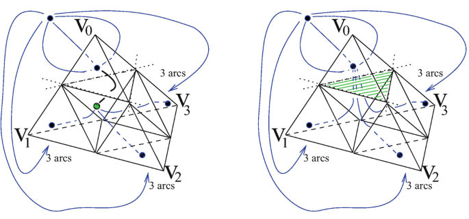
The (dual) graph \({\mathcal G}^2_*\) associated with the small mesh \({\mathcal M}_{all}\) defined in a tetrahedron T for r = 1: the black dots are the nodes, and curved lines the arcs (Left). The (dual) graph \({\mathcal G}^2\) obtained from \({\mathcal G}^2_*\) by merging the nodes corresponding to barycenter of t 0 = {(1, 0, 0, 0), T} and of O, thus eliminating the arc associated with the shaded small face \(f^O_{u}\) (Right)
Fig. 4 
Example of spanning tree in the (dual) graph \({\mathcal G}^2\), namely a selection of acyclic paths made of arcs, visiting all the nodes of \({\mathcal G}^2\) (r = 1, Left and r = 2, Right)
-
or t ◇, t ∘ have a small face on the boundary of the same octahedron O, i.e. f ◇ = ∂t ◇∩ ∂O and f ∘ = ∂t ∘∩ ∂O for the same octahedron O.


See an example of graph \({\mathcal G}^2\) for \({\mathcal M}_{all}\) (here \({\mathcal M} = \{T\}\)) in the left part of Fig. 3 for r + 1 = 2, where the node associated with the octahedron O is not a node in the graph, but stands to indicate that the four small tetrahedra are connected one to the other by one arc because they all have one small face on ∂O. Naming t k the small tetra with a vertex in v k, k = 0, 3, and numbering first the 3 × 4 faces on t k ∩ ∂T, called \(f^k_i\) for i = 1, 2, 3, second those on ∂O (where \(f^O_u\), \(f^O_\ell , f^O_d, f^O_r \) are the small faces up, left, down, right of ∂O), we have
Since the octahedron O is not part of the small mesh \({\mathcal M}_{all}\), we have to imagine that its node collapses with the node of one of its neighbouring small tetrahedron, say t 0 with a vertex in v 0, and thus that the corresponding arc (i.e. the small face \(f^O_{u}= \partial t_0 \cap \partial O\), the dashed one in the right part of Fig. 3) is eliminated. From a matrix point of view, D is obtained by adding the line “O” in D tmp to the line “t 0”, and eliminating \(f^O_{u}\), namely

(in bold font, the submatrix of maximal rank in D for the spanning tree \({\mathcal T}^2_s\) illustrated in Fig. 4, left part for r + 1 = 2). To repeat this construction in the two-dimensional case, when T is a triangle, we have to consider the mesh \({\mathcal M}_{all}\) of small triangles in T and the role of the core octahedra O is played by the reversed triangles ∇∈ T. The set \({\mathcal R}_2\) is replaced by \({\mathcal R}_1\), composed of one small edge for each reversed triangle \(\nabla \in {\mathcal K}_1\). In two dimensions we do not have reversed tetrahedra, therefore no reversed triangles ∇⊥.

(Left) In thick colored line, the small edges of the graph \({\mathcal G}^1\), for r = 3, that compose a spanning tree in a reference triangle. (Right) In thick blue line the contribution of the branches of a spanning tree in a (2D) toy mesh \({\mathcal M}\) reported on \({\mathcal M}_{all}\). In green, the contribution of the small branches mapped from the green ones in the reference triangle. It is not necessary to report the red ones since they are either covered by the blue ones or omitted. The co-tree is in black
The construction of the spanning tree in \({\mathcal M}_{all}\) can be done by assembling that of the geometrical mesh \(\mathcal M\), namely a spanning tree for the Whitney forms of lower degree (blue lines in Fig. 5 (Right)), together with local contributions, one from each element (green lines in Fig. 5 (Right)). Each local contribution results from one fixed on a reference element which is mapped on the current element (respecting the orientation). In Fig. 5 (Left), in green/red thick line we have marked the small edges of a spanning tree in the graph \({\mathcal G}^1\), for r = 3, in the reference triangle. The red ones belong to the spanning tree in the reference triangle, but they are in general omitted in the spanning tree of \({\mathcal M}_{all}\), (indeed, they appear only if they are covered by the blue tree). The small co-tree is in black. A similar construction can be repeated in 3D (both for k = 1 and k = 2) and it reflects the decomposition given, for instance, in [15] (Sect. 5).
References
Alonso Rodríguez, A., Rapetti, F.: The discrete relations between fields and potentials with high order Whitney forms. In: Radu, F.A., et al. (eds.) European Conference on Numerical Mathematics and Advanced Applications. Enumath 2017. Lecture Notes in Computational Science and Engineering LNCSE, vol. 126. Springer, Berlin (2018)
Alonso Rodríguez, A., Valli, A.: Finite element potentials. Appl. Numer. Math. 95, 2–14 (2015)
Alonso Rodríguez, A., Camaño, J., Ghiloni, R., Valli, A.: Graphs, spanning trees and divergence-free finite elements in domains of general topology. IMA J. Numer. Anal. 37, 1986–2003 (2017)
Amrouche, C., Bernardi, C., Dauge, M., Girault, V.: Vector potentials in three-dimensional nonsmooth domains. Math. Methods Appl. Sci. 21, 823–864 (1998)
Arnold, D., Falk, R., Winther, R.: Finite element exterior calculus, homological techniques, and applications. Acta Numer. 15, 1–155 (2006)
Bossavit, A.: Computational Electromagnetism: Variational Formulations, Complementarity, Edge Elements. Academic, New York (1998)
Bossavit, A., Rapetti, F.: Geometrical localization of the degrees of freedom for Whitney elements of higher order. IEE Proc. Science, Meas. Technol. 1/1, 63–66 (2007); Special Issue on “Computational Electromagnetism”
Cantarella, J., DeTurck, D., Gluck, H.: Vector calculus and the topology of domains in 3-space. Am. Math. Mon. 109, 409–442 (2002)
Christiansen, S.H., Rapetti, F.: On high order finite element spaces of differential forms. Math. Comput. 85/298, 517–548 (2016)
Girault, V., Raviart, P.A.: Finite Element Methods for Navier-Stokes Equations: Theory and Applications. Springer, New York (1986)
Nédélec, J.C.: Mixed finite elements in \(\mathbb {R}^3\). Numer. Math. 35, 315–341 (1980)
Rapetti, F., Bossavit, A.: Whitney forms of higher degree. SIAM Numer. Anal. 47/3, 2369–2386 (2009)
Rapetti, F., Dubois, F., Bossavit, A.: Discrete vector potentials for non-simply connected three-dimensional domains. SIAM Numer. Anal. 41/4, 1505–1527 (2003)
Stillwell, J.: Classical Topology and Combinatorial Group Theory. Springer, New-York (1993)
Zaglmayr, S.: High Order Finite Element Methods for Electromagnetic Field Computation. Ph.D. Thesis, Johannes Kepler Universität Linz, 2006
Author information
Authors and Affiliations
Corresponding author
Editor information
Editors and Affiliations
Rights and permissions
Open Access This chapter is licensed under the terms of the Creative Commons Attribution 4.0 International License (http://creativecommons.org/licenses/by/4.0/), which permits use, sharing, adaptation, distribution and reproduction in any medium or format, as long as you give appropriate credit to the original author(s) and the source, provide a link to the Creative Commons license and indicate if changes were made.
The images or other third party material in this chapter are included in the chapter's Creative Commons license, unless indicated otherwise in a credit line to the material. If material is not included in the chapter's Creative Commons license and your intended use is not permitted by statutory regulation or exceeds the permitted use, you will need to obtain permission directly from the copyright holder.
Copyright information
© 2020 The Author(s)
About this paper

Cite this paper
Rodríguez, A.A., Rapetti, F. (2020). Small Trees for High Order Whitney Elements. In: Sherwin, S.J., Moxey, D., Peiró, J., Vincent, P.E., Schwab, C. (eds) Spectral and High Order Methods for Partial Differential Equations ICOSAHOM 2018. Lecture Notes in Computational Science and Engineering, vol 134. Springer, Cham. https://doi.org/10.1007/978-3-030-39647-3_47
Download citation
DOI: https://doi.org/10.1007/978-3-030-39647-3_47
Published:
Publisher Name: Springer, Cham
Print ISBN: 978-3-030-39646-6
Online ISBN: 978-3-030-39647-3
eBook Packages: Mathematics and StatisticsMathematics and Statistics (R0)