Accelerator Operations

Abstract

The cost of building a particle accelerator is a major capital investment. Commissioning should be swift and the subsequent exploitation of a facility must provide an effective return. This return may be difficult to quantify unambiguously but generally acceptable measures of performance can be established. These measures might include: machine availability; integrated luminosity; protons on target; beam hours to users and so on.

Coordinated by M. Lamont.

9.1 Introduction

M. Lamont

The cost of building a particle accelerator is a major capital investment. Commissioning should be swift and the subsequent exploitation of a facility must provide an effective return. This return may be difficult to quantify unambiguously but generally acceptable measures of performance can be established. These measures might include: machine availability; integrated luminosity; protons on target; beam hours to users and so on.

The role of accelerator operations is to maximize the performance of an accelerator or accelerator complex by: minimizing downtime; maximizing the amount of beam delivered to the users; fully optimizing the quality of beam delivered to the users; and doing it all safely.

Accelerators and the control of particles beams have advanced considerably over recent years. There is deep understanding of particle dynamics, innovative measurement techniques, in-depth simulation and modelling, and widespread leverage of twenty-first century technology. It is not possible to go into too much depth here, instead some fundamentals that have been established from experience are outlined. References are given to more detailed sources. Some key operational considerations are outlined below and addressed in more detail in this chapter.

• Availability Accelerators are complex and their operations demands interfacing to a wide number of systems. Some these may be regarded as technical services e.g. cooling; cryogenics; electricity distribution. Others will have a more direct relationship with beam based operation e.g. power converters; radio frequency systems; beam instrumentation. One main challenge is to maintain the facility in a operable state for the maximum amount of time. Preventative maintenance, consolidation, fault tracking and fast problem resolution are required. In larger complexes there can be a chain of dependencies from sources, linacs and so on. Availability will be the cross product of the whole chain and associated primary services. Mean time between failure of essential components have to be evaluated at the design stage and appropriate component reliability assured. An effective fault tracking system is essential to identify weaknesses and targets for improvement.

• Reproducibility One key operational driver is reproducibility. In terms of the magnetic machine this implies careful attention to the powering history via a well defined pre-cycling strategy in a collider or careful cycle configuration in a fast cycling machine. A on-line measurement of the dipole field in a dedicated reference magnet system may be required. Reproducibility and stability of orbit can be critical for a number of reasons including guaranteeing collimator hierarchy or available aperture. Reproducibility of machine settings is to be expected and must be guaranteed.

• Control The control system will act as the primary interface to the accelerator systems and provide the means to communicate with a sub-system components. It will also provide high level facilities for driving the accelerator through its duty cycle. Although sometimes taken for granted, poorly designed controls can have a debilitating effect on the operability of an accelerator. Careful evaluation of the requirements and sufficient resources for development are required. Flexibility is required for commissioning and machine studies; access to control functionality and measurements for non-standard development should be considered.

• Instrumentation Effective beam instrumentation underpins control, optimization and understanding. The importance of well specified, reliable, accurate systems with appropriate acquisition systems and software cannot be understated.

• Optimization and stability The high performance demanded of modern machines can demand operating within tight parameter envelopes. Appropriate flexibility and precision in parameter control should be anticipated. Feedback systems for control of the key beam parameters can become mandatory. These could range from orbit and tune to transverse feedback systems. Harnessing modern technology and techniques is vital and again, expert resources must be given over to ensuring appropriate solutions. Commissioning these systems early in the lifetime of a machine should be a priority.

• Understanding Accelerator operations offers almost infinite possibilities for empirical tweaking as a way around problems. There is no substitute for building up real understanding of the key properties of a machine. These might include aperture, optics, instabilities, beam losses, beam and luminosity lifetimes. Good control and instrumentation are the tools of this trade and their importance is again stressed.

• Safety High energy and high power machines bring with them a number of risks. These risks have to be properly understood and protected against. For a complex machine the process of understanding the risks and their, sometimes, subtle interplay can be a painstaking process. Failure to perform this process properly can prove costly.

9.2 Parameter Control

The high level control system shall provide the following functionality:

• monitoring, recording and logging of accelerator status and process parameters;

• display of operator information regarding the accelerator status and beam parameters;

• operational settings management should provide facilities for the settings changes of all individual equipment systems; all settings changes shall be recorded, with simple-to-use roll-back possibilities;

• automatic process control and sequence control during all beam related modes of operation and covering all operational scenarios i.e. control within normal operating limits;

• prevention of automatic or manual control actions which might initiate a hazard;

• detection of the onset of a hazard and automatic hazard termination (e.g. dump the beam), or mitigation (e.g. establish control within safe operating limits).

In particular, control of the key beam parameters is vital to maintain good beam lifetime and minimize beam loss at all stages of operation. A general operational principle is to effect control at the appropriate level. Thus high level parameters such tune, chromaticity, synchrotron tune, bucket area, phase advance should used where appropriate. Software provides the appropriate translation to lower level hardware parameters such as current and voltage. The results of more complex beam dynamics analyses such as beta beating measurement and correction or the measurement and correction of non-linear effects have also to be incorporated in a sensible way into the machine settings.

9.2.1 Magnetic Elements

For a given machine configuration, optics programs are generally used off-line to generate the baseline settings in normalized strength for magnetic elements. These strengths should be imported into the settings management system and be amenable to adjustment as required. The required beam momentum is used to calculate the field or gradient required in a magnet or series of magnets.

For example, the required quadrupole gradient given a normalized quadrupole strength is calculated via Eq. (9.1).

$$\displaystyle \begin{aligned} k_2 = \frac{e}{p} \frac{\mathrm{d}B_z}{\mathrm{d}x} = \frac{1}{B\rho}\frac{\mathrm{d}B_z}{\mathrm{d}x}~. \end{aligned} $$

(9.1)

Given a required field or gradient in a magnet circuit the next challenge is to establish the required current to be supplied to the circuit. The two forms of Eq. (9.1) reflect the two main approaches to the challenge of conversion from required field or gradient to current.

The first approach depends on precise knowledge of the instantaneous total bending field in a synchrotron. This information can be obtained from a closed-loop measurement system, which generates and distributes a train of impulses (“B-train”) representing the field in a reference unit powered in series with the machine, or by a mathematical field model (“synthetic B-train”) possibly supplemented by off-line measurements. The real-time measurements of the main dipole field are then distributed to the power supply front-ends which perform a conversion from required gradient to current. Several major uncertainty sources apply in these cases, namely: temperature drifts, hysteresis behaviour in the iron, eddy current effects, material ageing [1].

An alternative, used at LEP and the LHC, is an off-line approach. Here look-up tables (gradient/field versus current) are pre-generated and used directly in the calculation of magnet currents, usually at the higher level of the control system. The LHC developed a semi-empirical model (“FiDeL” [2]) to generate the look-up tables and a description of the dynamic behaviour of multipole field errors. This model was based on a large database of test results which included all magnetic elements. The measurements were statistically analysed to extract model parameters. The required momentum is the taken as the driving parameter in the settings generation software; the current in all magnetic circuits is then given by pushing the required fields and gradients through the look-up tables.

9.2.2 Transverse Beam Parameters

Tune adjustment can be made using either the main quadrupoles circuits or dedicated trim quadrupole circuits. In the linear approximation it is straightforward to pre-calculate the coefficients relating strength changes to a given tune change. The key point here is to have on-line a rapid and easily available conversion between a beam parameter, magnet strength and ultimately power supply current. Once established the method can be used by on-line, off-line and real-time software.

The coefficients can either be established from standard definitions involving Twiss parameters or by pre-calculating the corresponding coefficients using, say, MADX, and use them with appropriate linear scaling to calculate the required changes in quadrupole strengths. The same arguments hold for all other commonly used operational parameters.

For chromaticity a matrix equation can be formed for the required change in sextupole strength given a desired change in chromaticity. Operationally the matrix coefficients can be pre-calculated either via the standard integrals or a machine model and then used on-line. Different sextupole families are often used in colliders to target different sources of chromaticity. Correction algorithms can be configured to weight different families as required.

Correction of the coupling can be important for machine performance and beam diagnostics. Sources of coupling include: tilted quadrupoles; solenoid fields; and vertical orbit deviations in sextupoles. Anticipating these sources at the design stage ensures that appropriately placed families of skew quadrupoles can be used to correct all sources of coupling. In principle the coupling generated by experimental solenoids and its correction can be pre-calculated. Correction of coupling from random sources in the machine can either be performed empirically or by compensating the coupling driving terms extracted from multi-turn BPM measurements. Knobs to correct the real and imaginary part of the coupling driving terms should be anticipated.

An effective method of measuring coupling is required. Methods range from measurements of the cross-plane tune amplitudes; the closest tune approach; measuring the cross-plane effects of beam excitation. More sophisticated measurement techniques can identified local sources of coupling and local correction may be possible if dedicated elements are available e.g. correction of coupling arising from tilts of the inner triplet magnets in the LHC. On-line methods using the transverse damper in AC-dipole mode to obtain spectral data around ring have provided automatic on-line correction of the real and imaginary parts of the coupling in the LHC.

The principles of orbit correction are described later in this chapter. Orbit dipole kicks should be treated as a parameter like any other. Thus

$$\displaystyle \begin{aligned} \theta_i = \frac{\Delta B \Delta s}{B \rho} \bigg|{}_i \end{aligned} $$

(9.2)

where θ _i is an orbit kick at a location s _i would slot into a settings management system in a consistent way, along with the use of orbit correctors in predefined local bumps and the like.

9.2.3 Generalization

The parameter space of a particle accelerator can be complex and large and might include the parameters such as tune, chromaticity and orbit but also others such as: Landau damping octupoles; bunch length control with wigglers; compensation of eddy current effects; higher order multipole correction with dedicated magnets etc. In a machine with an energy ramp these parameters and required corrections will be a function of time.

It should be easy to define combinations of parameters to give other higher level parameters (a “knob” in CERN parlance). These knobs can be then manipulated to control the ensemble. A simple example is a closed orbit bump. A more sophisticated example would be an optics correction which could include quadrupole strength adjustments and tune compensation.

Reliable settings management is mandatory. Generic tools for tracking all changes to settings should be deployed providing a full record of all settings changes. Archive and roll back facilities are essential. It is important that all parameter control be dealt within the same parameter and settings management system.

Besides the provision of tools for standard operations, the requirements of machine studies and commissioning should be borne in mind. Exploiting the machine in study mode often required non-standard measurements and non-standard control actions on accelerator hardware. An appropriate scripting environment (e.g. Python) with interfaces to control system functionality should allow the user to fully exploit the potential of the hardware and control system in a flexible and experimental way. Many of the tools thus developed can subsequently be incorporated into the standard operational environment. At the LHC this has included, for example, tools for beta beating measurement and correction, detection and logging of beam instabilities etc.

9.3 Orbit Correction

The main role of orbit correction is to centre the trajectory (in a transfer line) or the closed orbit (in a ring) inside the aperture or the magnetic elements, typically quadrupoles or wiggler magnets. This is usually achieved using global correction algorithms acting on all or a large part of the accelerator. In some cases local excursions may be desired, requiring the use of local ‘bumps’ of the orbit or trajectory.

9.3.1 Global Orbit Correction

Consider a storage ring with M beam position monitors (BPM) and N correctors. Orbit displacements $\vec {d}$ (M-component vector) arising from corrector kick angles $\vec {\theta }$ (N-component vector) are determined by the M × N linear response matrix A,

$$\displaystyle \begin{aligned} \begin{array}{rcl} \mathbf{A} \vec{\theta} &\displaystyle =&\displaystyle \vec{d}~, {} \end{array} \end{aligned} $$

(9.3)

$$\displaystyle \begin{aligned} \begin{array}{rcl} A_{mn} \! &\displaystyle =&\displaystyle \! \frac{ \sqrt{\beta _{m} \beta _{n} }}{2\,\sin \pi \nu } \, \cos \left( \left| \phi _{m} - \phi _{n} \right| - \pi \nu\right) . \end{array} \end{aligned} $$

(9.4)

The elements of A may be obtained from the machine model or be determined experimentally by measuring the deviation at each BPM resulting from exciting each corrector individually.

The task of the orbit correction is to find a set of corrector kicks $\vec {\theta }$ that satisfy the following relation,

$$\displaystyle \begin{aligned} \vec{d} + \mathbf{A} \vec{\theta} = 0 \; . \end{aligned} $$

(9.5)

In general the number of BPMs (M) and the number of correctors (N) are not identical and Eq. (9.5) is either over- (M > N) or under-constrained (M < N). In the former and most frequent case, Eq. (9.5) can not be solved exactly. Instead, an approximate solution must be found, and commonly used least square algorithms minimize the quadratic residual

$$\displaystyle \begin{aligned} S = \| \vec{d} + \mathbf{A} \vec{\theta} \|{}^2 \; . \end{aligned} $$

(9.6)

9.3.2 SVD Algorithm

When M ≥ N, the Singular Value Decomposition (SVD) [3] of matrix A has the form A = UWV ^t,

$$\displaystyle \begin{aligned} A = \left[ \begin{array}{cccc} u_{1}^{(1)} & u_{1}^{(2)} & \cdots & u_{1}^{(N)} \\ u_{2}^{(1)} & u_{2}^{(2)} & \cdots & u_{2}^{(N)} \\ \vdots & \vdots & & \vdots \\ u_{M}^{(1)} & u_{M}^{(2)} & \cdots & u _{M}^{(N)} \end{array} \right] \, \left[ \begin{array}{c} w_{1} \quad \quad \quad \quad \quad \quad \\ \quad w_{2} \quad \quad \quad \quad \quad \\ \quad \quad \quad \ddots \quad \quad \quad \\ \quad \quad \quad \quad \quad w_{N} \quad \end{array} \right] \, \left[ \begin{array}{cccc} v_{1}^{(1)} & v_{2}^{(1)} & \cdots & v_{N}^{(1)} \\ v_{1}^{(2)} & v_{2}^{(2)} & \cdots & v_{N}^{(2)} \\ \vdots & \vdots & & \vdots \\ v_{1}^{(N)} & v_{2}^{(N)} & \cdots & v_{N}^{(N)} \end{array} \right] . {} \end{aligned} $$

(9.7)

U is the M × N matrix whose column vectors $\vec {u}^{(\alpha )},\ (\alpha = 1, \ldots , N)$ form an orthonormal set, U ^t U = I. W is N × N diagonal matrix with non-negative elements. V ^t is the transpose of the N × N matrix V, whose column vectors $\vec {v}^{(\alpha )},\ (\alpha = 1, \ldots , N)$ form an orthonormal set, V ^t V = VV ^t = I.

From Eq.(9.7), it follows that (α = 1, …, N),

$$\displaystyle \begin{aligned} \mathbf{A} \vec{v} ^{(\alpha )} =w_{\alpha } \vec{u} ^{(\alpha )}, \quad {\mathbf{A}}^{t} \vec{u} ^{(\alpha )} = w_{\alpha } \vec{v} ^{(\alpha )} , \end{aligned} $$

(9.8)

and

$$\displaystyle \begin{aligned} \mathbf{AA}^{t} \vec{u} ^{(\alpha )} =w_{\alpha }^{2} \vec{u} ^{(\alpha )} , \quad {\mathbf{A}}^{t} \mathbf{A} \vec{v} ^{(\alpha )} = w_{\alpha }^{2} \vec{v} ^{(\alpha )} . \end{aligned} $$

(9.9)

When none of the diagonal elements w _α vanish, the solution of Eq.(9.5) is $\vec {\theta } = -\mathbf {VW}^{-1}{\mathbf {U}}^t \vec {d}$. $\vec {d}$ may be expanded in terms of eigenvectors $\vec {u}^{(\alpha )}$ [4],

$$\displaystyle \begin{aligned} \vec{d}\;=\;\sum_{\alpha =1}^{N}C_{\alpha } \vec{u} ^{(\alpha )} + \vec{d_0}~, \end{aligned} $$

(9.10)

where $C_\alpha = \vec {d} \cdot \vec {u}^{(\alpha )}$, while $\vec {d_0}$ corresponds to the uncorrectable part of the orbit. The corrector strength required for correction is

$$\displaystyle \begin{aligned} \vec{\theta}\;=\;-\sum_{\alpha =1}^{N}\, \frac{C_{\alpha } }{w_{\alpha } } \, \vec{v} ^{(\alpha )}~. {} \end{aligned} $$

(9.11)

If a given w _α = 0 indicating that the matrix is singular, one discards the corresponding term from Eq. (9.11). An example for an eigenvalue spectrum is given in Fig. 9.1 for LEP.

Fig. 9.1

Vertical orbit eigenvalue spectrum for LEP. The last four eigenvalues correspond to singular solutions in the low-beta sections around the interaction points

In practice one may want to limit the number of eigenvalues used for the correction to control the r.m.s. strength of the orbit correctors or to avoid small eigenvalues that are very sensitive to the accuracy of the model.

The SVD algorithm is ideally suited for feedback application since the correction can be cast in the simple form of a matrix multiplication once the SVD decomposition has been performed. This provides a fast and reliable correction procedure for realtime orbit feedback.

9.3.3 MICADO Algorithm

MICADO [5] is a least square correction algorithm based on Householder transformations. MICADO performs an iterative search for the most effective corrector and is, together with SVD, one of the most common orbit correction algorithms. For a non-singular matrix, a MICADO correction with all N correctors and an SVD correction with all N eigenvectors yield identical solutions. For corrections with a limited number of correctors or eigenvectors, and for singular matrices, the two algorithms converge differently.

A major difference between SVD and MICADO is the corrector strength distribution, MICADO using fewer but also much stronger kicks. The corrector strength r.m.s. can be easily controlled with SVD over the number of eigenvalues that are included in a correction. A correction of a small number of localized kicks is very effectively handled by MICADO, particularly when the response matrix is accurate, in which case MICADO can be used to identify the sources of the kicks. On the other hand, corrections based on few eigenvectors with the largest eigenvalues are similar to corrections of the main harmonics. Such a scheme spreads out the correction of a few kicks over the whole machine which can be an asset when the strength of correctors is limited. To compensate an isolated kick locally, a large number of eigenvectors must be included in the correction such that the linear combination forming $\vec {\theta }_c$ converges to a single nonzero corrector.

Singularities of the response matrix, associated to very small eigenvalues, are handled more easily with SVD, since it is sufficient to avoid using the corresponding eigenvectors in the corrections procedure. For the MICADO algorithm, it is necessary to regularize matrix A by removing redundant correctors.

9.3.4 Local Orbit Bumps

A local bump may be build from three correctors with deflections θ _1,2,3 at locations 1, 2, 3. The deflections may be expressed in terms of the lattice parameters,

$$\displaystyle \begin{aligned} \begin{aligned} \frac{\theta _{2} }{\theta _{1} } &\,=\, -\sqrt{\frac{\beta _{1} }{\beta _{2} } } \; \frac{\sin (\phi _{3} -\phi _{1} )}{\sin (\phi _{3} -\phi _{2} )}~, \\ \frac{\theta _{3} }{\theta _{1} } &\,=\, - \sqrt{\frac{\beta _{1} }{\beta _{3} } } \, \frac{\sin (\phi _{2} -\phi _{1} )}{\sin (\phi _{2} -\phi _{3} )}~. \end{aligned} \end{aligned} $$

(9.12)

At a target point t between 1 and 2, the position and angular displacements are

$$\displaystyle \begin{aligned} \begin{aligned} d_{t} &=&& \theta _{1} \sqrt{\beta _{1} \beta _{t} } \, \sin (\phi _{t}-\phi _{1} )~, \\ d_{t}^{\prime} &=&& \theta _{1} \sqrt{\frac{\beta _{1} }{\beta _{t} } } \, \big[ \cos \left( \phi _{t} -\phi _{1} \right) -\alpha _{t} \sin \left( \phi _{t} -\phi _{1} \right) \big]~. \end{aligned} \end{aligned} $$

(9.13)

At a point t between 2 and 3,

$$\displaystyle \begin{aligned} \begin{aligned} d_{t} &=&& \theta _{3} \, \sqrt{\beta _{3} \beta _{t} } \,\sin \left( \phi _{3} -\phi _{t} \right)~, \\ d_{t}^{\prime} &=&& - \theta _{3} \sqrt{\frac{\beta _{3} }{\beta _{t} } } \, \big[ \cos \left( \phi _{3} -\phi _{t} \right) +\alpha _{t} \sin \left( \phi _{3} -\phi _{t} \right) \big]~. \end{aligned} \end{aligned} $$

(9.14)

To control both position d _t and angle $d^{\prime }_t$ at the source point, a four-magnet local bump is required. The four-magnet local bump with corrector locations 1, 2, 3, 4, where the source point t is located between correctors 2 and 3 is given in terms of optics functions by:

$$\displaystyle \begin{aligned} \begin{aligned} \theta_{1} &=&& \frac{d_t \left( \cos{}(\phi_t - \phi_2) - \alpha_t \sin{}(\phi_t - \phi_2) \right)}{\sqrt{\beta_t \beta_1} \sin{}(\phi_2 - \phi_1)} - \frac{d^{\prime}_t \sqrt{\beta_t / \beta_1} \sin{}(\phi_t - \phi_2)}{\sin{}(\phi_2 - \phi_1)}~, \\[6pt] \theta_{2} &=&& \frac{-d_t \left( \cos{}(\phi_t - \phi_1) - \alpha_t \sin{}(\phi_t - \phi_1)\right)}{\sqrt{\beta_t \beta_2} \sin{}(\phi_2 - \phi_1)} + \frac{d^{\prime}_t \sqrt{\beta_t / \beta_2} \sin{}(\phi_t -\phi_1)}{\sin{}(\phi_2 - \phi_1)}~, \\[6pt] \theta_{3} &=&& \frac{-d_t \left( \cos{}(\phi_4 - \phi_t) - \alpha_t \sin{}(\phi_t - \phi_4)\right)}{\sqrt{\beta_t \beta_3} \sin{}(\phi_4 - \phi_3)} + \frac{d^{\prime}_t \sqrt{\beta_t / \beta_3} \sin{}(\phi_t -\phi_4)}{\sin{}(\phi_4 - \phi_3)}~, \\[6pt] \theta_{4} &=&& \frac{d_t \left( \cos{}(\phi_3 - \phi_t) - \alpha_t \sin{}(\phi_t - \phi_3)\right)}{\sqrt{\beta_t \beta_4} \sin{}(\phi_4 - \phi_3)} - \frac{d^{\prime}_t \sqrt{\beta_t / \beta_4} \sin{}(\phi_t - \phi_2)}{\sin{}(\phi_4 - \phi_3)}~. \end{aligned} \end{aligned} $$

(9.15)

9.3.5 Software

To be operationally useful the above algorithms must be fully integrated into application software. The software should typically provide the following functionality:

• an interface to orbit and trajectory acquisition system;

• the ability to compare measured orbits with saved references;

• the ability to calculate orbit corrections with a range of correction strategies (correction algorithm, number of correctors, number of eigenvalues) and send resulting correction to the machine;

• the ability to introduced a fully configurable local bump into the machine;

• facilities for dispersion measurement, harmonic analysis, energy offset analysis;

• facilities for threading, averaging and correction of the first N turns, injection point correction;

• multi-turn capture and analysis facilities.

9.4 Beam Feedback Systems

The domain of control system design is too vast to be comprehensively and briefly covered and thus this section focuses only on the key aspects that are applicable to accelerator control. The inclined reader is referred for a more detailed introduction to [6]. One distinguishes two paradigms that are used to drive and stabilise any given beam parameter:

• Feed-Forward which relies on the knowledge of the transfer function between beam parameter, required current and corresponding effective magnetic field, and essentially consists of inverting the scalar or matrix relations discussed in Sect. 9.3, and for matrices most commonly done using a Singular-Value-Decomposition based approach[7]. While this scheme is often sufficient, its intrinsic weakness of being limited by inaccuracies of the magnet’s transfer function, dynamic field effects such as e.g. the decay- and snapback phenomenon in superconducting magnets and random external perturbations may lead to a potentially out-of-tolerance systematic error Δ𝜖 = 1 − 𝜖, which is illustrated as a difference between the reference and actual beam process variable in Fig. 9.2a. Still, this type of control is suitable for many beam parameters such as the beam momentum where the magnet and RF transfer functions involved are typically known on the 0.1% level.

  Fig. 9.2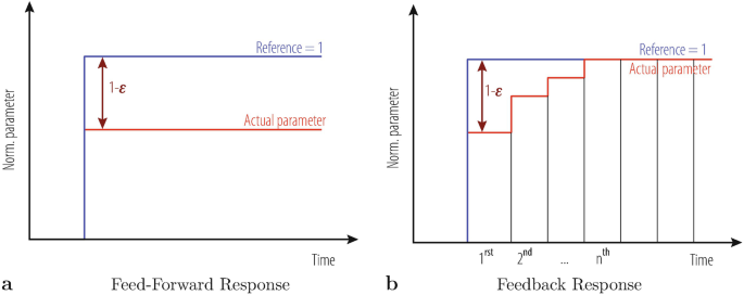

  

  Feed-forward and feedback signal in response to a step reference change: the actual value of process variable and residual errors 1-𝜖 are indicated and vanishes to zero in case of an integral feedback

• Feedback may be used in case the beam parameter model is insufficient (due to, for example, multiple dependencies or random perturbations) and at the same time the parameter deviations being accessible by beam instrumentation or diagnostics methods. In this case, the corresponding measurements can either be used to: (a) improve the knowledge of the beam parameter to magnetic field to current transfer function (feed-forward scheme), or (b) to ‘feed back’ part of the measured value into the reference that is send to the magnets or RF systems. In this case the difference Δ𝜖 = 1 − 𝜖 drives a controller that iteratively optimises the actuator signal by minimising Δ𝜖 till the actual beam process variable matches the desired reference value as shown in Fig. 9.2b. Due to intrinsic limitations such as the bandwidth of the magnetic circuits and non-linear effects such as delays and rate-limits, the stabilisation is typically not instantaneous. To cope with these effects requires a more complex form of controller to optimise temporal convergence.

The strength of feedbacks is that they require, in comparison to feed-forward systems, only a rough process model while reducing the residual error through continuous adjustments or measure-and-correct iterations. For a steady-state scenario, the final parameter stability is ultimately limited by the noise and systematic error of the underlying beam parameter measurement. Since the robustness and stability of the beam instruments directly translates through this into the robustness and stability of the feedback loop, a good understanding of the underlying instrument, measurement and diagnostic principles is of paramount importance while designing beam-based feedback systems.

Two types of feedback are often distinguished: those acting within a given accelerator cycle (e.g. during injection, acceleration, store, dump) and those acting on a cycle-to-cycle basis where the disturbance measurements of the previous cycle are used to drive the actual state.¹ Both cases are similar and differ mainly on the time-scale in between measurements and corrections, the latter offers less strict requirements in terms of read-out speed and bandwidth of the involved beam instrumentation’s acquisition system and is often initially favoured to a continuous read-out. The basic measurement, control principles and issues remain the same however.

9.4.1 Feedback Controller Design

A simple loop block diagram consisting of a single-input-single-output (SISO) beam response G(s) and controller D(s) is shown in Fig. 9.3. Here, r is the desired beam parameter reference, y the actual parameter state, e the feedback error being the difference between both, and u the output that is generated by the controller that minimise the error within the given constraints (e.g. response time, required power, etc.). One distinguishes typically at least three different error sources that can enter the feedback system: internal perturbations δ _i that are amplified by the same beam transfer function G(s) as the to be stabilised parameter, external perturbations δ _d and measurement noise δ _m that while not directly affecting the actual state y may propagate to it depending on the choice of controller function D(s). Depending on whether the system is implemented in the analogue or digital domain, it is convenient to transform the differential or difference equations of controller and beam process transfer functions using the Laplace² or Z-Transform. Both transforms translate complex convolutions in time domain to simple multiplications in the s- or z-domain. For the sake of simplicity, further discussion uses the Laplace transform but equally applies to Z-transformed digital systems.

Fig. 9.3

First order closed loop block diagram

For low-order beam parameters—such as orbit, tune, coupling, chromaticity and energy—the effects of the RF and individual corrector circuits are usually sufficiently linear and thus G(s) is often approximated by a scalar K or matrix transfer function as described in Sect. 9.2 followed by a given time dependence. The time dependence of most electrical magnet circuits and RF systems is well approximated as first- (low-pass) and second-order (simple harmonic oscillator) systems with transfer functions given as:

$$\displaystyle \begin{aligned} \begin{array}{rcl} G_{\text{first order}}(s) &\displaystyle =&\displaystyle \frac{K}{\tau s + 1}~, {} \end{array} \end{aligned} $$

(9.16)

$$\displaystyle \begin{aligned} \begin{array}{rcl} G_{\text{second order}}(s) &\displaystyle =&\displaystyle \frac{K \omega_0^2}{s^2 + 2\zeta\omega_0 \cdot s + \omega_0^2}~, {} \end{array} \end{aligned} $$

(9.17)

with τ being the constant of the low-pass characteristic, ζ the damping factor and ω ₀ the eigenfrequency of the system. In an ideal world the feed-forward (M(s) = 0) controller design would try to achieve a unity gain system transfer function

$$\displaystyle \begin{aligned} T_{\mathrm{open\mathrm{-}loop}}(s) := D(s) G(s) \rightarrow 1 {}~, \end{aligned} $$

(9.18)

which for a perfect actuator response corresponds to inverting Eqs. (9.16) and (9.17). However, in a real-world environment this can be only be achieved for reference changes with limited time-constants due to intrinsic limits on the power converter’s slew-rate. Also, any scaling error in D(s) or modelled G(s) would yield a static error on the actual parameter output and discussed before.

If part of the actual parameter value is measured via a monitor transfer function M(s), compared to the reference and the difference fed into the controller it is useful to define the following transfer functions that describe the stability and sensitivity to perturbations and noise

$$\displaystyle \begin{aligned} \begin{array}{rcl} T(s) &\displaystyle :=&\displaystyle \frac{y}{r} = \frac{D(s)G(s)}{1+D(s)G(s)}~, {} \end{array} \end{aligned} $$

(9.19)

$$\displaystyle \begin{aligned} \begin{array}{rcl} S_{d}(s) &\displaystyle :=&\displaystyle \frac{y}{\delta_d} = \frac{1}{1+D(s)G(s)}~, {} \end{array} \end{aligned} $$

(9.20)

$$\displaystyle \begin{aligned} \begin{array}{rcl} S_{i}(s) &\displaystyle :=&\displaystyle \frac{y}{\delta_i} = \frac{G(s)}{1+D(s)G(s)}~, {} \end{array} \end{aligned} $$

(9.21)

$$\displaystyle \begin{aligned} \begin{array}{rcl} S_{u}(s) &\displaystyle :=&\displaystyle \frac{u}{\delta_d} = \frac{D(s)}{1+D(s)G(s)}~, {} \end{array} \end{aligned} $$

(9.22)

where T(s) is the nominal closed-loop (feed-back) transfer function, S _d(s) the nominal sensitivity defining the loop disturbance rejection, S _i(s) the input-disturbance sensitivity and S _u(s) the control sensitivity. The state variables are indicated in Fig. 9.3.

It can be easily see, inserting Eq. (9.18) into 9.19, that using the same ideal open-loop controller relation described above in a closed-loop would yield a loop response error of 50% even for a perfect system. However, assuming only a perfect scalar controller D(s) = D ₀ on can see that the loop response converges to one for larger controller gain D ₀ and in particular becomes less dependent on relative errors of G(s) which again illustrates the advantages of feed-back over feed-forward systems. However, at the same time one can show that the transfer function between actual beam parameter and measurement noise is equal to the nominal transfer function $T(s) = \frac {y}{\delta _m}$. Thus while simply increasing the scalar gain D ₀ yields a perfect loop response to reference changes, it also causes the system to propagate any measurement error directly onto the actual beam parameter.

Thus, from the beam diagnostics point of view, in case the given instrument is to be used in beam-based feedbacks, the involved instrumentation performance is sometimes prematurely optimised—often including significant filtering in M(s) to reduce the measurement noise—prior to closing the feedback loop. While this is suitable for systems that are used for verification or monitoring only, it has certain disadvantages when used in feedbacks e.g. through introducing additional sampling delays. Combining the filtering of beam instruments and closed-loop responses inside D(s) is not just equivalent to this from a noise point of view but also improves the feedback response by minimising the total loop delay in these cases.

The discussed simple scalar controller are usually only used if the beam parameter response is much faster than the required reference changes (e.g. feedback that act on a cycle-to-cycle basis) but need to be extended for time dependent components for the other cases. Classic feedback designs typically rely on the discussion of denominator zeros in Eqs. (9.19) and (9.20) while keeping constraints such as required bandwidth, minimisation of overshoot, limits on the maximum possible excitation signal and robustness with respect to model and measurement errors. For ideal processes, this yields adequate controller designs but often falls short in providing a simple comprehensive method for estimating and modifying the loop sensitivity (robustness) in the presence of process uncertainties, non-linearities and noise.

Here, Youla’s affine parameterisation method for optimal controllers is briefly introduced, which is based on the analytic process inversion, first introduced in [8]. For an open-loop stable process G(s), the nominal closed-loop transfer function is stable if and only if Q(s) is an arbitrary stable proper transfer function and D(s) parameterised as:

$$\displaystyle \begin{aligned} D(s) = \frac{Q(s)}{1-Q(s)G(s)}~. {} \end{aligned} $$

(9.23)

The stability of the closed loop system follows immediately out of the above definition if inserted into Eqs. (9.19)–(9.22). The sensitivity functions in the Q(s) form are given as:

$$\displaystyle \begin{aligned} \begin{array}{rcl} T(s) &\displaystyle =&\displaystyle Q(s)G(s)~, {} \end{array} \end{aligned} $$

(9.24)

$$\displaystyle \begin{aligned} \begin{array}{rcl} S_{d}(s) &\displaystyle =&\displaystyle 1-Q(s)G(s)~, {} \end{array} \end{aligned} $$

(9.25)

$$\displaystyle \begin{aligned} \begin{array}{rcl} S_{i}(s) &\displaystyle =&\displaystyle (1-Q(s)G(s))G(s)~, {} \end{array} \end{aligned} $$

(9.26)

$$\displaystyle \begin{aligned} \begin{array}{rcl} S_{u}(s) &\displaystyle =&\displaystyle Q(s)~. {} \end{array} \end{aligned} $$

(9.27)

Assuming G(s) is stable, the only requirement for closed loop stability is for Q(s) to be stable. The strength of this method is the explicit controller design with respect to required closed loop performance, as visible in Eq. (9.24), and required stability (Eqs. (9.25)–(9.27)). Equations (9.24) and (9.25) are complementary and illustrate the intrinsic limiting trade-off of feedbacks that either have a good disturbance rejection or are robust with respect to noise. The ultimate limit is thus defined rather by the bandwidth and noise performance of the corrector circuits and beam measurements than by the feedback loop design itself.

9.4.1.1 First and Second Order Example

The design formalism can be demonstrated using a simple first order system $G_0(s)=\frac {K_0}{\tau \cdot s + 1}$ with open-loop gain K ₀ and time constant τ. A common controller design ansatz is to write Q(s) as

$$\displaystyle \begin{aligned} Q(s)=F_Q(s)\cdot G_0^{i}(s)~, {} \end{aligned} $$

(9.28)

with F _Q(s) a trade-off function and $G_0^{i}(s)$ the pseudo-inverse of the process. Since G ₀ does not contain any unstable zeros, the pseudo-inverse equals the inverse and is given by $G_0^{i}(s):= [G_0(s)]^{-1}=\frac {\tau \cdot s+1}{K_0}$. Q(s). In order for D(s) to be biproper, F _Q(s) must have a degree of one and can be written as:

$$\displaystyle \begin{aligned} F_Q(s) = \frac{1}{\alpha s+1}~. {} \end{aligned} $$

(9.29)

Inserting Eq. (9.28) into Youla’s controller parameterisation equation (9.23) yields the following controller:

$$\displaystyle \begin{aligned} D(s) = \frac{\tau}{K_0 \alpha} + \frac{1}{K_0 \alpha s} = K_p + K_i\cdot\frac{1}{s}~, \end{aligned} $$

(9.30)

which shows a simple PI controller structure with proportional gains K _p and integral gain K _i. Inserting Eq. (9.28) into (9.24) yields

$$\displaystyle \begin{aligned} T_0(s) = F_Q(s) \end{aligned} $$

(9.31)

that the closed loop response is essentially determined by the choice of trade-off function F _Q(s) and that the closed loop bandwidth is proportional to the parameter 1∕α. This can be used to tune the closed loop between: high disturbance rejection but high sensitivity to measurement noise (small α) and low noise sensitivity but low disturbance rejection (large α) depending on the operational scenario. The maximum possible closed loop bandwidth is limited by the excitation, as described by Eq. (9.27). In case of power converters, for example, the excitation is limited by the maximum available voltage.

One can derive a similar optimal controller for a second-order system (Eq. (9.17)) using a similar ansatz:

$$\displaystyle \begin{aligned} Q(s) = F_Q(s) \cdot G^i(s) = \frac{\omega_{cl}^2} {s^2 + 2\zeta_{cl}\omega_{cl}`s + \omega_{cl}^2} \cdot G^i(s) \end{aligned} $$

(9.32)

yields the following controller PID structure

$$\displaystyle \begin{aligned} D(s) = K_p + K_i \cdot \frac{1}{s} + K_d \cdot \frac{s}{\tau_d s +1} \end{aligned} $$

(9.33)

with proportional gains K _p, integral gain K _i and integral gain K _d defined as:

$$\displaystyle \begin{aligned} \begin{array}{rcl} K_p &\displaystyle =&\displaystyle \frac{4\zeta_{cl}\zeta_0\omega_0\omega_{cl}-\omega_0^2}{{4K_0\zeta_{cl}^2}}~, \end{array} \end{aligned} $$

(9.34)

$$\displaystyle \begin{aligned} \begin{array}{rcl} K_i &\displaystyle =&\displaystyle \frac{\omega_0^2\omega_{cl}} {2K_0\zeta_{cl}}~, \end{array} \end{aligned} $$

(9.35)

$$\displaystyle \begin{aligned} \begin{array}{rcl} K_d &\displaystyle =&\displaystyle \frac{4\zeta^2\omega_{cl}^2-4\zeta_0\omega_0\zeta_{cl}+\omega_0^2}{{8K_0\zeta_{cl}^3\omega_{cl}}}~,~~\mathrm{with}~~ \tau_d = \frac{1}{2\zeta_{cl}\omega_{cl}}~. \end{array} \end{aligned} $$

(9.36)

There are several options but the most commonly used discrete ‘velocity form’ of above PID controller (without contracting sums) can be written as

$$\displaystyle \begin{aligned} u[n] &= u[n-1] + K_p \cdot \left(e[n]-e[n-1]\right) + K_i \cdot T_s \cdot e[n] \\ &+ \frac{K_d}{T_s}\cdot\left(e[n]-2e[n-1]+e[n-2]\right) \end{aligned} $$

(9.37)

with n being the sampling index, T _s the sampling frequency, u[n] the controller output and e[n] the measured error signal. The error signal e[n] that is specifically used for the last differential part of the controller is nearly always low-pass filtered to suppress high-frequency noise that is common in discrete systems and that would otherwise be amplified by the K _d term. Compared to analogue feedbacks, digital feedbacks are more robust and their operation more reproducible compared to cases where temperature drifts or other external factors would affect analogue controller. Thus, in case the requested bandwidths are in the few Hz to MHz-range, digital feedbacks are the de-facto standard. Still, digital controllers are fundamentally limited by the intrinsic phase-lag caused by the sampling and dynamic range due to the finite number of ADC bits available at that frequency. Thus for feedbacks operating in the range of a few hundred to GHz range or where a high dynamic range is required, analogue feedbacks are still used. In any case, neither fully analogue nor fully digital representations are exact, and the final implementation is usually validated using beam-based optimisation techniques.

9.4.1.2 Non-linear Systems

The same method can be extended to open-loop unstable and multi-input-multi-output (MIMO) systems [8]. Real life feedbacks may contain significant delays λ (due to e.g. data transmission, data processing etc.) and non-linearities G _NL(s), due to e.g. saturation and rate limits of the corrector circuits’ power supplies. The modified process can be written, for example as:

$$\displaystyle \begin{aligned} G(s) = G_0(s)\cdot e^{-\lambda s} G_{NL}(s)~. {} \end{aligned} $$

(9.38)

Using the same pseudo-inverse $G_0^{i}(s)$ as for the above example and inserting Eq. (9.28) into (9.23) yields a controller parameterisation D _NL(s) including a classic Smith-Predictor and anti-windup paths, discussed in more detail in [6, 9]. Inserting Eq. (9.28) including the delay and non-linearities into Eq. (9.24) yields the following closed loop transfer function:

$$\displaystyle \begin{aligned} T(s) = F_Q(s) \cdot e^{-\lambda s} G_{NL}(s)~. \end{aligned} $$

(9.39)

Similar to the linear case discussed above, the closed loop is essentially defined by the function F _Q(s) that within limits can be chosen arbitrarily based on the required disturbance rejection and robustness during possibly different operational scenarios (gain-scheduling). Further information and a review on Youla’s parameterisation can be found in [6, 10].

9.4.2 Inter-Loop Dependencies

Above described individual parameter control complexity is dwarfed by the challenge of operating parallel feedback loops on for example orbit, tune, chromaticity, coupling, radial position and transverse bunch-by-bunch motion. Even in a fully optimised scheme, some cross-talk is inevitable: the momentum modulation required to measure chromaticity induces tune and radial offsets that are seen by the tune, orbit and radial position feedbacks; transverse feedback, by design, minimises the very same beam oscillations required to measure the tune. If not addressed at an early design stage, a naïve one-by-one implementation of these feedback loops can lead to serious interferences, coupling and instabilities.

There are various classic de-coupling strategies such as: diagonalisation, e.g decoupling of horizontal and vertical planes; suppression of known cross-terms, i.e. allowing certain variations which are required for measurements; dead-bands to limit the operational ranges of one feedback in favour of another; time-scheduling between feedback actions, such as alternating tune measurements with transverse feedback operation; choosing different bandwidths for each loop.

An improved de-coupling strategy is to derive the dependent variable from the compensated feedback actuator control signal. In this case the tune feedback is operated at the maximum desired bandwidth, fully compensating radial modulation induced tune changes. Chromaticity is in turn derived and corrected from the amplitude of the actuator signal required to stabilise the tunes. Due to the finite bandwidth and gain of the feedback, the actuator signal does not typically contain the full modulation. An accurate chromaticity estimate needs to account for this and should be complemented by the demodulation of the residual tune frequency oscillation remaining on the beam. The required dispersion orbit variation and corresponding momentum mismatch need to be addressed differently. This is done by subtracting them dynamically from the orbit and radial-loop feedback reference targets. In machines running with transverse feedback systems, the tune can similarly be derived from its actuator signal while keeping beam oscillations and potential instabilities under control. Because of the various inter-loop dependencies, it is beneficial to implement the tune, chromaticity, coupling, orbit and radial-loop feedbacks in one global controller to minimise data exchange and synchronisation requirements.

9.5 Optics Measurement and Correction

9.5.1 Introduction

The unavoidable misalignments and field errors of the different components of an accelerator cause distortions of the machine optics with respect to the design. Optics errors deteriorate the accelerator performance and can even challenge the machine safety when operating with beam. Optics measurement and correction techniques are therefore fundamental to keep optics errors as low as possible or within specified tolerances [11]. The following sections review procedures and techniques to measure and correct various optics parameters, focusing on circular accelerators.

9.5.2 Optics Measurement Techniques

The tune is probably the most fundamental optics parameter as resonances need to be avoided for efficient accelerator operation. One- and two-dimensional resonance lines in the tune space have correspondances to Farey sequences [12]. The fractional part of the tune, Q, is given by the frequency of the beam oscillations when sampled turn-by-turn at any longitudinal location s,

$$\displaystyle \begin{aligned} z(N)=\sqrt{2J\beta(s)}\cos\big(2\pi QN+\phi(s)+\phi_0\big) \ , {} \end{aligned} $$

(9.40)

where z stands for horizontal or vertical position and J and ϕ ₀ are the amplitude and phase invariants of the beam oscillations. Exciting the beam oscillations above the frequency noise floor of the Beam Position Monitors (BPMs) is crucial for the tune measurement. All optics measurements involve some kind of excitation as discussed below.

9.5.2.1 Quadrupole Strength Modulation

A change in the integrated strength of a quadrupole ΔKL yields a change in the tunes ΔQ _x,y that can be unambiguously used to determine the average β _x,y functions over the quadrupole [13],

$$\displaystyle \begin{aligned} \overline{ \beta }_{x,y} = \pm\frac{2}{\Delta KL}\Big( \cot{}(2\pi Q_{x,y})\big( 1-\cos{}(2\pi\Delta Q_{x,y}) \big) + \sin{}(2\pi\Delta Q_{x,y}) \Big) \approx \pm4\pi\frac{\Delta Q_{x,y}}{\Delta KL}\ , {} \end{aligned} $$

(9.41)

where the ± sign refers to the horizontal and vertical planes, respectively. The approximation displayed to the right of Eq. (9.41) is applicable for 2π ΔQ _x,y ≪ 1 and Q _x,y far away from the integer and the half-integer. This technique is routinely used in many synchrotrons [14,15,16,17,18]. Hadron colliders typically operate with Q _x very close to Q _y. In this case a good correction of coupling is required prior to measurements with quadrupole strength modulation.

9.5.2.2 Closed Orbit Distortion

Exciting an orbit corrector with a deflection strength of Δθ yields a closed orbit distortion around the ring given by

$$\displaystyle \begin{aligned} \Delta x_{co}(s)=\Delta\theta\frac{\sqrt{\beta(s)\beta(s_0)}\cos\big(|\phi(s)-\phi(s_0)|-\pi Q\big)}{2\sin\pi Q}~, \end{aligned} $$

(9.42)

where s is the location of the BPM and s ₀ is the location where the kick (Δθ) is applied. The β(s) and ϕ(s) functions can be obtained at the BPMs as the result of fitting to a collection of orbit distortions induced by, at least, three different orbit correctors per plane, as done in KEKB [19]. Closed orbit distortions are also the basis of another optics measurement and correction algorithm [20, 21] where quadrupole strengths and other machine parameters are fitted to reproduce a large ensemble of closed orbit acquisitions. This has demonstrated very effective in synchrotron light sources, however its application to large scale machines as the LHC requires unaffordable long times for measurements and computer calculations.

9.5.2.3 Betatron Oscillations, Free or Forced

The phase of the turn-by-turn free betatron oscillations, see Eq. (9.40), can be directly used to compute phase advances between pairs of nearby BPMs. The amplitude of the betatron oscillations can be used to measure β functions but it requires a good control of the BPM calibration errors [22,23,24]. Instead the phase advances between three or more BPMs can be used to obtain β and α functions as described in [25,26,27].

The Fast Fourier Transform (FFT) of the BPM signal, z(N), offers a poor resolution on the phase measurement. Interpolated FTs like [28] or Singular Value Decomposition (SVD) algorithms like [29] feature a higher performance in terms of spectral resolution. The achievable resolution is usually limited by decoherence processes that damp the bunch centroid oscillations. Furthermore, beam decoherence also affects FT amplitudes and phases, which can be partially restored [30, 31, 42]. These limitations can be overcome by forcing betatron oscillations with the aid of an AC dipole with a frequency close to the machine tune. Moreover, if the AC dipole is ramped up and down adiabatically the beam emittance is preserved [32, 33].

The beam dynamics with forced oscillations features remarkable differences from that of free oscillations [34,35,36,37]. In presence of an AC dipole the measured β functions differ from the machine β functions. This difference is simply modelled as a quadrupole error of strength KL _ac in the location of the AC dipole [38], where KL _ac is given by

$$\displaystyle \begin{aligned} KL_{ac}=\pm2\frac{\cos{}(2\pi Q_{x,y})-\cos{}(2\pi Q_{ac})}{\beta_{ac}\sin{}(2\pi Q_{x,y})} \approx \pm4\pi\frac{Q_{ac}-Q_{x,y}}{\beta_{ac}}\ , \end{aligned} $$

(9.43)

where the ± sign refers to the horizontal and vertical planes, respectively. This equivalence allows to apply exactly the same analysis to all experimental data but using a modified reference model which includes the quadrupole error according to the AC dipole settings.

9.5.2.3.1 Transverse Momentum Reconstruction

It is convenient to study the transverse phase space using normalized coordinates, $\hat {z}(N)=z(N)/\sqrt {\beta }$. The turn-by-turn transverse normalized momentum, $\hat {z}'(N)=-\sqrt {2J}\sin \big (2\pi QN+\phi (s)+\phi _0\big )$, can be reconstructed by using the normalized signal from two BPMs, $\hat {z}_1(N)$ and $\hat {z}_2(N)$, as

$$\displaystyle \begin{aligned} \hat{z}^{\prime}_1(N)=\Big( \hat{z}_2(N) - \hat{z}_1(N)\cos{}(2\pi\Delta_{12}) \Big)/\sin{}(2\pi\Delta_{12})\ , \end{aligned} $$

(9.44)

where Δ₁₂ is the phase advance between the two BPMs. If non-linear elements are placed in between the two BPMs extra contributions to $\hat {z}^{\prime }_1(N)$ appear as described in [39].

9.5.2.3.2 Coupling Measurement

Using the complex variable, $h_z(N)=\hat {z}(N)-i\hat {z}'(N)$, the turn-by-turn motion in presence of linear coupling is given by [40]

$$\displaystyle \begin{aligned} \begin{aligned} h_x(N) &=&\!\!\! \sqrt{2J_x}e^{i\phi_x(N)}- i2f_{1001}\sqrt{2J_y}e^{i\phi_y(N)} -i2f_{1010}\sqrt{2J_y}e^{-i\phi_y(N)}~,\\[3pt] h_y(N) &=&\!\!\! \sqrt{2J_y}e^{i\phi_y(N)}- {} i2f_{1001}^*\sqrt{2J_x}e^{i\phi_x(N)} -i2f_{1010}\sqrt{2J_x}e^{-i\phi_x(N)}~, \end{aligned} \end{aligned} $$

(9.45)

where ϕ _x,y(N) = 2πNQ _x,y + ϕ _x0,y0 and f ₁₀₀₁ and f ₁₀₁₀ are the coupling difference and sum resonance terms, respectively. These terms are linearly related to the elements of the coupling matrix as described in [41]. All the monomials in the right-hand-side of Eqs. (9.45) correspond to a single spectral line of the complex spectrum with frequencies ± Q _x and ± Q _y. By applying a complex FT to the h _x,y variables as reconstructed from the BPMs it is possible to measure the amplitude and phases of the coupling terms. To achieve a measurement independent of BPM calibration and beam decoherence, the values obtained from the horizontal and vertical planes are geometrically averaged as described in [42]. The closest tune approach, ΔQ _min, can be computed from the skew quadrupolar fields as [13],

$$\displaystyle \begin{aligned} \Delta Q_{\mathrm{min}}=\left|\frac{1}{2\pi}\oint{\mathrm{d}s\ j(s)\sqrt{\beta_x\beta_y} e^{-i(\phi_x-\phi_y)+i({Q}_x-{Q}_y)s/R}}\right|\ , \end{aligned} $$

(9.46)

where j(s) is the skew quadrupolar gradient around the ring and R is the machine radius. ΔQ _min can also be computed from the difference resonance term f ₁₀₀₁ around the ring by [43,44,45]

$$\displaystyle \begin{aligned} \begin{array}{rcl} \Delta Q_{\mathrm{min}} &\displaystyle =&\displaystyle \left| \frac{4({Q}_x-{Q}_y)}{2\pi R} \oint \mathrm{d}s f_{1001} \mathrm{e}^{-i(\phi_x-\phi_y)+i({Q}_x-{Q}_y)s/R} \right| \end{array} \end{aligned} $$

(9.47)

$$\displaystyle \begin{aligned} \begin{array}{rcl} &\displaystyle \approx &\displaystyle \left| 4({Q}_x-{Q}_y) \overline{ f_{1001} \mathrm{e}^{-i(\phi_x-\phi_y)} } \right| \lesssim 4\left|{Q}_x-{Q}_y\right| \overline{ \left|f_{1001}\right| }\ ,{} \end{array} \end{aligned} $$

(9.48)

where $\overline { x }$ represents the ring average of x. Linear coupling in combination with octupolar fields gives rise to an amplitude dependent closest tune approach [46, 47].

9.5.2.3.3 Measurement of Non-linearities

Betatron oscillations are also used to measure resonance driving terms f _jklm since these affect the motion as follows [40]

$$\displaystyle \begin{aligned} h_x(N)\,{=}\, \sqrt{2J_x}e^{i\phi_x(N)}\,{-}\, i2\sum_{jklm}\!jf_{jklm}(2J_x)^{\frac{j+k-1}{2}}(2J_y)^{\frac{l+m}{2}} e^{i[(1-j+k)\phi_x(N)+(m-l)\phi_y(N)]}. \end{aligned} $$

(9.49)

First sextupolar resonance driving terms measurements and applications were carried out in [42], where the effects of beam decoherence on these measurements are also described. First resonance terms measurements using AC dipoles to avoid beam decoherence are described in [39].

9.5.2.4 Dispersion Measurement

Dispersion is typically inferred from the orbit change induced by a shift in the RF frequency, see e.g. [13]. This measurement is affected by the BPM calibration errors. Alternatively it is possible to measure the ratio $D_x/\sqrt {\beta _x}$ (normalized dispersion) independently of BPM calibration errors if $\sqrt {\beta _x}$ is inferred from the amplitude of the beam oscillations [48].

9.5.3 Optics Correction Techniques

The most used correction approach consists in building a response matrix R of the available machine variables on a collection of observables. For instance,

$$\displaystyle \begin{aligned} \begin{array}{rcl} \left( \Delta Q_x,\Delta Q_y, \frac{\vec{\Delta\beta_x}}{\beta_x}, \frac{\vec{\Delta\beta_y}}{\beta_y}, \Delta\vec{\phi}_x, \Delta\vec{\phi}_y, \Delta\frac{\vec{D_x}}{\sqrt{\beta_x} } \right)^T &\displaystyle =&\displaystyle {\mathbf{R}} \Delta\vec{k}^T~, \end{array} \end{aligned} $$

(9.50)

$$\displaystyle \begin{aligned} \begin{array}{rcl} \left( \Delta\mathfrak{R}\vec{f}_{1001}, \Delta\mathfrak{I}\vec{f}_{1001}, \Delta\mathfrak{R}\vec{f}_{1010}, \Delta\mathfrak{I}\vec{f}_{1010}, \Delta\vec{D}_y \right)^T &\displaystyle =&\displaystyle {\mathbf{R}}_s \Delta\vec{k}_s^T~, \end{array} \end{aligned} $$

(9.51)

where $\vec {k}$ stands for quadrupole strengths but also horizontal orbit bumps at the sextupoles and $\vec {k}_s$ represents skew quadrupoles or vertical orbit bumps at sextupoles. R and R _s are pseudo-inverted and applied to the measured deviations of the optics parameters to compute the effective corrections. The correction should incorporate appropriate weights as illustrated in [49]. The success of this approach strongly depends on the configuration of errors and available correctors. Sextupolar resonance driving terms have been successfully corrected using an equivalent approach in [50]. For large localized errors this approach tends to distribute the correction over many correctors around the machine.

9.5.3.1 Segment-by-Segment Technique

A more local approach, the segment-by-segment technique [51, 52], consists in splitting the machine into a collection of independent beam lines by using as starting optics parameters the measured $\beta _{x,y},\alpha _{x,y},D_{x,y},D^{\prime }_{x,y}, f_{1001}, f_{1010}$. The comparison of the measurements and the propagated optics parameters along the segment will reveal discrepancies starting at the error location. The local error sources or the effective corrections can be computed by means of matching algorithms using only the machine variables in the segment.

9.6 Longitudinal Control and Manipulations

H. Damerau and R. Garoby

H. Damerau R. Garoby

RF systems in synchrotrons are primarily installed for beam acceleration. However, they provide also the possibility to manipulate the longitudinal beam characteristics like bunch length, energy spread, distance between bunches, number of bunches, etc. [53]. The following section deals with the typical longitudinal beam manipulations in synchrotrons, when synchrotron radiation is negligible.

9.6.1 Adiabaticity

The longitudinal motion that we consider is conservative (i.e. there is no energy dissipation effect like synchrotron radiation, as well as no coupling of longitudinal and transverse motion). Liouville’s theorem is then applicable, which states that the local density of particles in the longitudinal phase plane is always constant [54]. The time scale for the rate of change is given by the oscillation frequency of the individual particles at the centre of a bunch:

$$\displaystyle \begin{aligned} \omega_s \propto \left(\frac{hV \cdot \eta \cos \phi_s}{\gamma}\right )^{\frac{1}{2}}~, \end{aligned} $$

(9.52)

where h is the RF harmonic number, V  the RF voltage, φ _s the stable phase and η the slip factor ($\eta = 1/\gamma ^2 - 1/\gamma _t^2$). If the rate of change of the accelerator parameters is slow enough for the distribution of particles to be continuously at equilibrium in the longitudinal phase plane, longitudinal emittance is preserved [55]. Such a process is called “adiabatic”. The degree of adiabaticity is assessed by the adiabaticity parameter ε. It is defined as the relative change of the synchrotron frequency, ω _s, during one period:

$$\displaystyle \begin{aligned} \varepsilon = \frac{1}{\omega_{s}^{2} } \left | \frac{d \omega_s}{dt} \right |~. \end{aligned} $$

(9.53)

Adiabatic processes can be reversed in time.

9.6.2 Changing the Longitudinal Characteristics of the Bunches

When a process is slow enough to be quasi-adiabatic (ε < 0.1), the particle distribution is completely determined by the instantaneous beam and accelerator parameters. The area occupied in the longitudinal phase plane (emittance) remaining constant, bunch length l _b (in ns) and energy spread ΔE _b (in eV) evolve like:

$$\displaystyle \begin{aligned} l_b \propto \frac{1}{\beta} \cdot \left( \frac{\eta}{\gamma \cdot hV \cos \varphi_s} \right)^{\frac{1}{4}}~, \end{aligned} $$

(9.54)

$$\displaystyle \begin{aligned} \Delta E_b \propto \beta \cdot \left( \frac{\gamma \cdot hV \cos \varphi_s}{\eta} \right)^{\frac{1}{4}}~. \end{aligned} $$

(9.55)

When the accelerator parameters (e.g. RF voltage or phase) are quickly varying, the process is non-adiabatic and tracking simulations are required to evaluate the final particle distribution. Although the local density of particles remains constant, the contour containing all particles is usually not a stable trajectory in the final state and the resulting emittance is therefore larger because of filamentation. Non-adiabatic beam manipulations allow getting bunch lengths and energy spreads which cannot be obtained with adiabatic processes (“bunch rotation”). They also give the possibility to blow-up the longitudinal emittance in a controlled fashion (“longitudinal controlled blow-up”).

9.6.3 Bunch Rotation

A step increase of the RF voltage triggers a “bunch rotation” in the longitudinal phase plane during which the bunch length first decreases during 1∕4 of a synchrotron period (Fig. 9.4a).

Fig. 9.4

Bunch rotation for bunch shortening. (a) 1∕4 a synchrotron period in the longitudinal phase plane after a fast voltage step; (b) bunch stretching prior to rotation by phase jump

A step decrease has the opposite effect of first lengthening the bunch. To achieve the smallest possible bunch length, as required, for example, for transferring the beam to the following synchrotron equipped with a higher frequency RF system, this two effects can be combined [56, 57].

Because the focusing voltage is sinusoidal, the rotated bunch has a marked S-shape if, at any moment during the process, its length has exceeded ≃ 1∕3 of an RF period. If very short bunches have to be obtained, the maximum tolerable length is even smaller [53]. More sophisticated techniques making use of multiple RF harmonics have been developed to improve the results [58].

To avoid the step increase in RF voltage, a phase jump by π of the RF voltage can be applied instead [59]. The bunch is stretched at the unstable point between two buckets (Fig. 9.4b). Switching the RF voltage back to its initial phase triggers the rotation in the longitudinal phase plane.

9.6.4 Longitudinal Controlled Blow-Up

Increasing the longitudinal emittance is a convenient mitigation means against instabilities by keeping the beam below threshold. Such a blow-up should not generate tails in the distribution of particles. The most efficient and fast technique makes use of a phase-modulated high frequency (V _H, h _H) superimposed to the RF holding the beam (h _rf ≪ h _H) [60, 61]:

$$\displaystyle \begin{aligned} V_H = \hat{V}_H \sin{}(h_H \omega_R t + \alpha \sin \omega_M t + \vartheta_H)~, \end{aligned} $$

(9.56)

α being the peak phase modulation, ω _R the modulation frequency and 𝜗 _H a phase constant. This high frequency phase-modulated voltage perturbs motion in the longitudinal phase plane. Resonances can be induced which create a re-distribution of density in the bunch. Parameters are in practice determined with computer simulations and finely adjusted on the real accelerator. Typical ranges of values are shown in Table 9.1. A smaller harmonic ratio h _H∕h _rf can also be used, although blow-up is then slower.

Table 9.1 Typical ranges of blow-up parameters

With RF voltage at a single harmonic controlled longitudinal blow-up is obtained by modulating either the voltage [62] or the phase [63] with noise, which introduces diffusion [64, 65]. To target specific parts of a bunch with the blow-up to shape its distribution, bandwidth limited noise can be applied.

9.6.5 Changing the Bunch Train

9.6.5.1 Iso-Adiabatic Rebunching (Debunching)

The simplest technique for bunching a continuous beam (e.g. a beam from a linac after it has debunched because of its energy spread) with a minimum emittance blow-up consists of applying an iso-adiabatic increase. With ω _s ∝ V ^1∕2 (Eq. (9.52)) the RF voltage function which keeps the adiabaticity ε constant (ε < 0.1) becomes (Fig. 9.5)

$$\displaystyle \begin{aligned} V(t) = \frac{V_I} { \left [1- \left (1-\sqrt{\frac{V_I}{V_F}} \right ) \frac{t}{t_F}\right ]^2}~, \end{aligned} $$

(9.57)

V _I being the initial RF voltage applied at the start of rebunching, and t _F the moment when the final RF voltage V _F is reached. The adiabaticity of the process is inversely proportional to its duration, ε ∝ 1∕t _F.

Fig. 9.5

Iso-adiabatic rebunching voltage

To minimize the emittance blow-up, V _I has to be low, typically such that the beam energy spread is significantly larger than the bucket height. However, for a given adiabaticity, the smaller V _I is, the smaller the initial synchrotron frequency and hence the slower the whole rebunching process.

Debunching is the inverse process to transform a bunched beam into a continuous beam. An iso-adiabatic voltage variation is also used, which is a time-reversed version of the one used for rebunching (Fig. 9.5).

9.6.5.2 Splitting (Merging)

Splitting is used to multiply the number of bunches by 2 or 3 and merging is the reverse process [66,67,68]. With respect to iso-adiabatic debunching-rebunching, these processes have the advantage of preserving gaps without beam and keeping the beam always under RF control. In theory as well as in practice, they can be quasi-adiabatic and almost without blow-up.

Splitting bunches in 2 can be obtained using two RF systems with an harmonic ratio of 2 [67]. The bunch is initially held by the first system (V ₁, h ₁) while the second (V ₂, h ₂ = 2h ₁) is stopped. The unstable phase on the second harmonic is centred on the bunch. As V ₂ is slowly increased and V ₁ decreased the bunch lengthens and progressively splits in two as illustrated in Fig. 9.6.

Fig. 9.6

Bunch splitting in two. (a) RF voltages vs. time; (b) longitudinal phase plane

Good results are consistently obtained when the voltage $V_1(h_1)=V_{1\_sep}$ is such that, at the moment when two separate bunches have just formed, the initial bunch would fill 1∕3 of the bucket acceptance in the absence of second harmonic (V ₂(h ₂) = 0). Linear voltage variations with a total duration larger than 5 synchrotron periods in the bucket ($V_{1\_sep}, h_1$) give satisfying results. Each final bunch has ideally 1∕2 the emittance of the initial one. Practically, less than 10% additional longitudinal emittance growth is achieved. The longitudinal bunch distribution is preserved during the process. Splitting is also obtained when applying an RF voltage at h ₂ > 2h ₁, resulting in empty buckets in between split bunches [69].

Splitting bunches in three requires three simultaneous RF systems on three harmonics [68]. A stable phase on the third harmonic (3h ₀) coincides with the stable phase on first one (h ₀) and with an unstable phase on the second harmonic (2h ₀). The voltage variations are computed for obtaining three equal bunches of 1∕3 the initial emittance. Voltages and evolution in longitudinal phase space as a function of time are illustrated in Fig. 9.7.

Fig. 9.7

Bunch splitting in three. (a) RF voltages vs. time; (b) longitudinal phase plane

9.6.6 Slip Stacking

Slip stacking is a non-adiabatic technique for combining bunches two by two [70, 71]. It is fast, but it leads to large emittance blow-ups. The two beams have to be held by two slightly different RF frequencies. If the frequency difference is large enough (Δω > 2ω _s, where ω _s is the synchrotron frequency in the centre of an unperturbed bucket of one family), two families of buckets coexist which drift towards each other because of their frequency difference (Fig. 9.8). Consequently, and provided the acceptance of the buckets is large enough (acceptance > 2 × emittance), the bunches drift with them and slip past each other. When they are superimposed in azimuth, pairs of bunches can be captured in large buckets centred at the middle frequency.

Fig. 9.8

Slip stacking: evolution in the longitudinal phase plane during the process

Although improvements are possible, like reducing the frequency difference towards the end of the process, the longitudinal contour enclosing a pair of bunches in the final bucket always contains a large area without particles. Therefore the emittance after filamentation is much more than doubled and longitudinal density is accordingly reduced.

9.6.6.1 Batch Compression (Expansion)

Batch compression does not change the number of bunches but concentrates them in a reduced fraction of the accelerator circumference [72]. It can be quasi-adiabatic and consequently avoids longitudinal emittance blow-up.

The principle is slowly to increase the harmonic number of the RF controlling the beam as shown in Fig. 9.9. Starting from harmonic h ₁, voltage is progressively increased on harmonic h ₂ > h ₁ and decreased on h ₁, until harmonic h ₂ finally holds the batch of bunches. The phase on h ₂ with respect to h ₁ must be such that bunches converge symmetrically towards the centre of the batch. This can be achieved for even (compression around unstable point between buckets) or odd number of bunches (central bucket does not move in phase).

Fig. 9.9

Batch compression (top to bottom) or expansion (bottom to top)

Due to the presence of RF voltage at two harmonics simultaneously during each harmonic number step, the effective RF voltage is amplitude modulated at the difference harmonic |h ₁ − h ₂|,

$$\displaystyle \begin{aligned} \begin{array}{rcl} {} V \! &\displaystyle =&\displaystyle \! V_1 \sin{h_1 \omega_R t} + V_2 \sin{h_2 \omega_R t} \\ \! &\displaystyle =&\displaystyle \! 2 V_0 \cos \left( \frac{h_1 + h_2}{2} \omega_R t \right) \cdot \sin \left( \frac{h_1 - h_2}{2} \omega_R t \right) \quad \mathrm{at} \quad V_0 = V_1 = V_2~.\quad \end{array} \end{aligned} $$

(9.58)

In case h ₁ and h ₂ have common dividers, the process repeats gcd(h ₁, h ₂) (gated common divider) times around the circumference, which allows to compress or expand multiple batches of bunches simultaneously.

The amount of compression achievable in a single step is limited by the acceptance of the buckets holding the edge bunches. A consequence is that multiple batch compression steps are necessary to reach large compression factors, and complicated manipulations of RF parameters are involved.

Non-linear voltage programs can be applied to improve the adiabaticity of the process [73].

9.7 Collimation

9.7.1 Introduction

The concept of a collimator and its design are introduced in [74]. The design process for a collimation system and several important issues are discussed in [75]. In this chapter we focus on the performance and operational use of a collimation system. We quickly introduce a few central definitions:

• A collimation system is an ensemble of collimators that is integrated into the accelerator layout to intercept stray particles and to protect the accelerator.

• Collimation is acting in the normalized phase space. With z = x or z = y, the Twiss functions β _z and α _z, and the emittance 𝜖 _z we define the normalized coordinates z _n and $z^{\prime }_{n}$ as:

  $$\displaystyle \begin{aligned} z_{n} = \frac{z}{\sqrt{\epsilon_{z}\beta_{z}}}~,~~ z^{\prime}_{n} = \frac{\alpha_{z}z + \beta_{z}z'}{\sqrt{\epsilon_{z}\beta_{z}}}~. \end{aligned} $$

  (9.59)

  It is noted that the transverse beam size (Gaussian rms) is given by $\sigma _{z}= \sqrt {\epsilon _{z}\beta _{z}}$.

• An unperturbed particle describes a circle in normalized phase space with amplitude:

  $$\displaystyle \begin{aligned} a_{z } = \sqrt{z_{n}^{2}+z_{n}^{'2}}~. \end{aligned} $$

  (9.60)

• Collimator settings from the beam are defined in normalized coordinates (numbers of beam size σ _z) with n ₁ being the collimator family setting closest to the beam, n ₂ the second closest setting, and so on. Several families usually define a hierarchy that must be respected. Often this results in stringent tolerances on the positioning of collimators.

9.7.2 Definition of Cleaning Efficiency and Performance

A collimation system is designed to intercept stray particles with maximum efficiency and thus to protect critical regions of the accelerator. Critical regions can be experiments that must be protected against background from beam halo, super-conducting magnets that must be protected against quenches or hands-on maintenance equipment that must be protected against activation from beam losses. A system with 100% efficiency would absorb all impacting particles and power with zero leakage into critical zones. However, the various nuclear processes in the collimator jaw materials will always cause some particles to escape the system. The creation of secondary and tertiary halo in a two-stage collimation system is illustrated in Fig. 9.10.

Fig. 9.10

Illustration of the secondary and tertiary halo created by a two-stage collimation system in vertical phase space (LHC example). The scattering along the jaw surface creates the characteristic lines of halo particles in phase space

9.7.2.1 Local Cleaning Inefficiency

For collimation it is convenient to define inefficiency or leakage [76]. We first introduce inefficiency and then connect it to efficiency. The inefficiency η _c of a collimation system with a primary collimation cut at n ₁ is defined as the ratio between the number N _leak of particles that leak out and reach a normalized transverse amplitude $a_{z}^{cut}$ and the number N _impact of impacting particles:

$$\displaystyle \begin{aligned} \eta_{c}=\frac{N_{leak} (a_{z}>a_{z}^{cut})} {N_{impact}}~. \end{aligned} $$

(9.61)

We require that $a_{z}^{cut} > n_{1}$. The value for a _z is given by the available machine aperture and is often around 10 sigma. Modern collimation systems can reach quite low inefficiencies with η _c in the range of 10⁻² (1%) to 10⁻⁴ (0.01%). Efficiency η can then be defined as η = 1 − η _c and is in the range of 99% to 99.99%.

Inefficiency is, however, not sufficient to characterize the performance of a collimation system. It is important to realize that the large amplitude particles are not lost at one location but are spread over some dilution length L _dil. For local losses we define a local cleaning inefficiency $\tilde {\eta }_c$ [76]:

$$\displaystyle \begin{aligned} \tilde{\eta}_c = \frac{\eta_c}{L_{dil}}~. \end{aligned} $$

(9.62)

Local cleaning inefficiency has a unit of 1/m. As the dilution is not uniform, simulations are used to predict the local cleaning inefficiency $\tilde {\eta }_{c}$ along the whole accelerator. This definition allows a direct comparison with measurements. Collimation systems must be designed to minimize local cleaning inefficiency. This is achieved by both minimizing global inefficiency (overall leakage) and maximizing dilution. It is crucial to work on both aspects for achieving best performance.

9.7.2.2 Performance Reach with Collimation

The overall performance of an accelerator is often limited by the peak residual loss that appears in one or few critical locations. It is therefore useful to define a maximum local cleaning inefficiency $\max [\tilde {\eta }_{c}]$ over all critical locations. For example, in a super-conducting storage ring $\max [\tilde {\eta }_{c}]$ describes the peak loss per m in super-conducting magnets. Alternatively, in a linac $\max [\tilde {\eta }_{c}]$ may describe the peak loss per m in the regions that must be protected for hands-on maintenance.

During the design phase one should define an allowable maximum beam loss rate R _lim for critical locations. The maximum allowed loss rate R _loss at the collimators is defined in particles per second. It depends on the allowable maximum beam loss rate R _lim for critical locations and the maximum local inefficiency of the system [76]:

$$\displaystyle \begin{aligned} R_{loss} = \frac{R_{lim}}{\max[\tilde{\eta}_c]}~. \end{aligned} $$

(9.63)

The loss rates R _loss can be converted into energy deposition rate P _loss using:

$$\displaystyle \begin{aligned} P_{loss} = \frac{R_{loss}}{\mbox{(p/s)}} \cdot \frac{E_b}{\mbox{(GeV)}} \cdot 1.6022 \times 10^{-10} \; \mbox{W}~. \end{aligned} $$

(9.64)

Considering a stored beam and assuming that all leaked particles are lost at collimators we can relate R _loss =  ΔN∕ ΔT to the number of particles N _max and beam lifetime τ _min:

$$\displaystyle \begin{aligned} \tau_{min} = - \frac{\Delta T}{\ln \left( 1 - \frac{R_{loss} \cdot \Delta T}{N_{max}} \right)} \approx \frac{N_{max}}{R_{loss}}~. \end{aligned} $$

(9.65)

For convenience we give the equation for calculating the energy deposition rate for any lifetime:

$$\displaystyle \begin{aligned} P_{loss} \approx N_{max} \cdot \frac{\mbox{(h)}}{\tau_{min}} \cdot \frac{E_b}{\mbox{(GeV)}} \cdot 4.45 \times 10^{-17} \; \mbox{kW}~. \end{aligned} $$

(9.66)

The maximum achievable beam intensity can be expressed as a function of the maximum local cleaning inefficiency, the minimum beam lifetime that must be sustained and the limit of beam loss in critical regions [76]:

$$\displaystyle \begin{aligned} N_{max} = \frac{\tau_{min} \cdot R_{lim}}{\max[\tilde{\eta}_c]}~. \end{aligned} $$

(9.67)

Similar equations can be given for single-pass accelerators. This equation can be used during the design phase of an accelerator to specify the required collimation performance once beam intensity, minimum beam lifetime and loss limits have been determined. A proper design of a collimation system requires a well-defined target for cleaning efficiency.

9.7.3 Operational Settings and Tolerances

Modern collimation systems are often designed to form a multi-stage cleaning system. The collimators then belong to different stages (families), where all collimators of a given stage sit at the same setting (in normalized coordinates). The system will only work correctly if the collimators fulfil the hierarchy requirement [77, 78]. For the example illustrated in Fig. 9.11 the following condition must be fulfilled for the collimation half gaps:

$$\displaystyle \begin{aligned} n_{1} < n_{2} < n_{3} < n_{\mbox{ triplet}} < n_{4} < n_{\mbox{ arc}}~. \end{aligned} $$

(9.68)

Fig. 9.11

Illustration of collimation hierarchy for the example of LHC collimation [79]. The system establishes global, multi-stage cleaning of halo particles. To be effective, the different collimator families must respect a strict hierarchy in normalized phase space

Typical values for the half gaps n ₁ to n ₄ are in the range of 5 σ _z to 10 σ _z. The differences in normalized settings are called collimator retractions Δx:

$$\displaystyle \begin{aligned} \begin{array}{rcl} \Delta x_{1} &\displaystyle =&\displaystyle n_{2}-n_{1}~, \\ \Delta x_{2} &\displaystyle =&\displaystyle n_{3}-n_{2}~,\\ \Delta x_{3} &\displaystyle =&\displaystyle n_{\mbox{ triplet}}-n_{3}~,\\ \Delta x_{4} &\displaystyle =&\displaystyle n_{4} - n_{\mbox{ triplet}}~,\\ \Delta x_{5} &\displaystyle =&\displaystyle n_{\mbox{ arc}}-n_{4}~. \end{array} \end{aligned} $$

(9.69)

The retraction values can become quite small. For example, in LHC at 7 TeV retraction values can be smaller than 1 σ _z. At the same time emittance at high energy becomes very small (0.5 nm for the LHC at 7 TeV) and the transverse beam size σ _z can be as small as 140 μm. The smallest collimator retraction values can therefore be in the range of 100 μm, imposing strict operational tolerances.

Various imperfections can reduce the available collimator retraction [78]:

• Beam loss deposits energy on the collimator jaws. The resulting heating can lead to transient jaw deformations.

• If off-momentum beta beating is not or insufficiently corrected, the retraction becomes a function of particle momentum and can be different for particles inside a bunch. See discussion in [74].

• Inaccuracies in beam-based set-up for collimators in different families. See discussion in next section.

• Drifts in beam orbit around the ring since last beam-based set-up or during the beam cycle (for example during squeeze in IP beta function). The possible impact on retraction is illustrated in Fig. 9.12. Most critical is a zero orbit change at a primary collimator and a maximum change at a secondary collimator.

  Fig. 9.12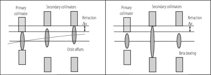

  

  Illustration of machine errors (top: orbit error; bottom: beta beating) that can affect the collimation hierarchy in normalized phase space and reduce cleaning efficiency

• Change in beta functions around the ring. The possible impact on retraction is illustrated in Fig. 9.12. Most critical is a reduction in beta function at primary collimators and an increase at secondary collimators.

A reduction in collimator retraction reduces the efficiency of the system (up to a factor 10 is possible [80]) and can render it operationally unstable. At some point a secondary collimator can start acting as a primary collimator and efficiency can suddenly be reduced by two orders of magnitude. A collimation system should always be quantified in terms of operational tolerances to make sure that it is appropriately designed and can deliver the required performance. Two sided collimators (as shown in the example of Fig. 9.12) are preferable for operational stability.

9.7.4 Beam-Based Set-Up of Collimation

The previous section explained the criticality of correct collimator hierarchy. It was shown that retraction values can be in the range of 100 μm. Collimators must be centred around the beam with an accuracy that is a fraction of the collimator retraction. Tolerances for collimator settings can then be in the range of a few 10’s of μm. However, the exact beam position and size are not known a priori with this accuracy. Collimators are therefore set up in a beam-based process. This beam-based procedure differs for one-pass or stored beams.

• In a single pass accelerator or in transfer lines a collimator jaw is moved through the beam [81,82,83]. This process is illustrated in Fig. 9.13. Initially (the jaw is still out of the beam) there is a transmission of 100% of beam intensity while downstream beam loss monitors (BLM’s) read zero (no showers from the collimator). When the jaw is cutting the beam in its centre then there is a transmission of about 50% and the BLM reads half of its maximum value. Finally, when the jaw intercepts the full beam, the transmission is almost zero and the BLM reads a maximum value, independent of the exact jaw position. This “collimator scan” method allows calibrating the beam centre and size. A related method establishes a collimation gap that is smaller than the beam size. This gap is then scanned across the beam. The transmission and beam loss signals are measured during the scan while recording the gap position. A precise determination of beam centre and size is possible.

  Fig. 9.13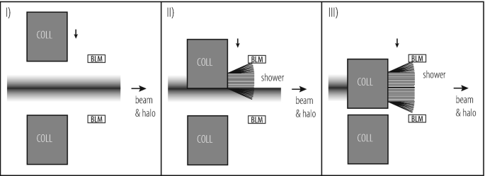

  

  Illustration of beam-based set-up of a collimator in a beam line with single pass beam. A collimator jaw is moved from out position (I) through a centre position (II) into a beam-intercepting position (III). The beam centre is inferred by (a) measurement of beam-induced showers with a beam-loss monitor and/or (b) by measurement of the not intercepted beam intensity

• In a storage ring the effects of phase space mixing and amplitude conservation are used, as shown in Fig. 9.14. Any collimator (most often a primary collimator) can be used to define a betatron cut in normalized phase space [77, 78, 81]. This can be done with a single jaw. Assuming zero dispersion, the same phase space cut is present all around the ring after phase space mixing (particles oscillating around the closed orbit, sweeping around the whole allowed phase space volume). The second jaw of the reference collimator can then be moved to the same cut. A sudden spike in beam loss measured downstream of the collimator is used to detect the halo edge. Successively all collimators around the ring are set up to the same cut in normalized phase space. In the end all jaws are centred on the beam and any beta variations have been calibrated. It is noted that the method is affected by systematic errors that must be taken into account. For example, each set-up will scrape the beam halo by a small additional amount δ. It is advisable to recheck the edge periodically with the reference collimator. Also, tilts in the collimator jaws can induce errors in the knowledge of the collimation gap which can limit the accuracy in determining local beam size.

  Fig. 9.14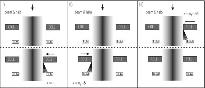

  

  Illustration of beam-based set-up of collimators in a ring with stored beam. At first a reference collimator is defined and one of its jaws is used to create an edge in the normalized beam shape (I). Phase space mixing establishes the same edge all around the ring, in positive and negative directions (in case of zero dispersion). Then the second jaw of the reference collimator is moved to the same normalized position by observing beam loss (II). Analogous, a jaw from any other collimator can be moved to the same defined beam cut (III)

Once collimators have been set up it is important to record all beam conditions, especially the orbit and optics of the accelerator. This information can then be used to re-establish the collimator set-up and hierarchy for extended periods of times. Collimator set-ups could be used and kept operational for up to 5 months without repeating a set-up for the LHC.

9.7.4.1 Measurement of Collimation Performance

Collimation performance can be measured if a distributed beam loss measurement system has been installed around the ring [84, 85]. Ideally beam loss is measured at all collimators [86, 87], all quadrupoles (here the beta functions are maximal) and other critical locations [88]. An example measurement of collimation performance in the LHC at 450 GeV is shown in Fig. 9.15. The procedure for such a measurement is described below.

• The measurement should not disturb the orbit or the beta functions, as this would decrease the cleaning efficiency. Therefore one induces a strong diffusion process that rapidly increases the beam emittance. In a storage ring one can move the beam onto a resonance, for example the $\frac {1}{3}$ resonance.

  Fig. 9.15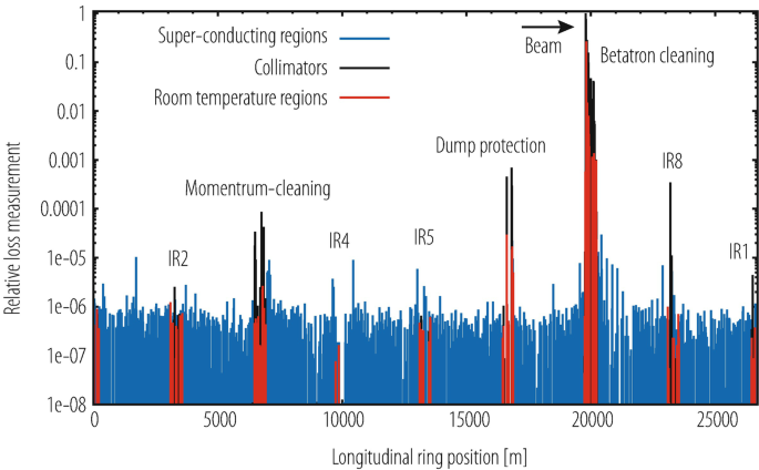

  

  Example for a measurement of collimation performance in the LHC at 450 GeV. The data shows peak integrated losses over 1.3 s. A beam loss is provoked for beam 1 in the horizontal plane. Losses are normalized to the peak loss in the ring. The peak loss appears as expected at the betatron collimators and falls off exponentially over the betatron cleaning insertion. Leakage around the ring is measured. The measurement resolution is limited by noise in the beam loss monitors (6 orders of magnitudes below the peak loss)

• The integrated beam losses are monitored around the ring as the beam emittance is blown up, for example with a 1.3 s integration time as shown in Fig. 9.15. The data with the highest losses is selected.

• The loss data is normalized to the highest loss all around the ring, which by definition should occur at a collimator. Losses at different locations are distinguished by colour.

The example in Fig. 9.15 shows the results that can be achieved when generating a rapid horizontal emittance blow-up for one beam. The relative loss measurement shown is very similar to the local cleaning inefficiency as defined above, if we ignore differences in BLM response and realize that measured losses are per BLM and not per meter. The measured maximum “local cleaning inefficiency” in a critical region (super-conducting magnets) is about 2 × 10⁻⁵, illustrating a very good performance. The collimators in the cleaning insertion and other areas in the ring intercept reliably all losses and leakage is very small.

9.8 Luminosity Optimization

9.8.1 Introduction

The performance of a collider can be characterized by three main parameters:

• the centre of mass collision energy E _CM (in the following we will assume two beams with equal beam energies → E _CM = 2 ⋅ E _beam);

• the instantaneous luminosity specifying the rate at which certain events are generated in the beam collisions (number of events per second = L(t) ⋅ σ _event with σ _event being the cross section of the event of interest);

• the integrated luminosity specifying the total number of events that are produced over a time interval t − t ₀.

The instantaneous luminosity is given by

$$\displaystyle \begin{aligned} L = \frac{f_{rev}\cdot n_{b}\cdot N_{1}\cdot N_{2}}{2\pi\sqrt{(\sigma^{2}_{x,1}+\sigma^{2}_{x,2})}\cdot\sqrt{(\sigma^{2}_{y,1}+\sigma^{2}_{y,2})}}\cdot F\cdot H, {} \end{aligned} $$

(9.70)

where f _rev is the revolution frequency, n _b the number of bunches colliding at the interaction point (IP), N _1,2 are the particles per bunch and σ _x,1,2 and σ _y,1,2 the horizontal and vertical beam sizes of the two colliding beams. F is the geometric luminosity reduction factor due to collisions with a transverse offset or crossing angle at the IP and H is the reduction factor for the hour glass effect that becomes relevant when the bunch length is comparable or larger than the beta functions at the IP (→ the transverse beta function varies over the luminous region where the two beams interact with each other).

In the following we assume that all bunches of both beams have equal intensities (N ₁ = N ₂ = N _b) and the same size at the IP. The transverse beam sizes at the IP are given by

$$\displaystyle \begin{aligned} \sigma_{x,y} = \sqrt{(\beta^{*}_{x,y}\cdot\epsilon_{x,y}) + D^{2}_{x,y}\cdot \delta^{2}_{p}}, {} \end{aligned} $$

(9.71)

where δ _p is the relative momentum spread ($\delta _{p} = \frac {\Delta p}{p_{0}}$) of the particles within a bunch, $\beta ^{*}_{x,y}$ and D _x,y are the horizontal and vertical beta and dispersion functions at the IP and 𝜖 _x,y the horizontal and vertical emittances of the two beams.

Because the bunch intensities and beam sizes of a collider vary over time, the instantaneous luminosity is implicitly a function of time.

The integrated luminosity is defined by

$$\displaystyle \begin{aligned} \hat{L}(t-t_{0}) = \int_{t_{0}}^{t} L(\tau) d\tau, \end{aligned} $$

(9.72)

where t ₀ is an arbitrary starting point, L(τ) the instantaneous luminosity at a given time and t − t ₀ the time period of interest.

Optimizing the luminosity of a collider aims essentially at two goals:

• maximize the total number of events over a given time interval → maximize the integrated luminosity;

• minimize the experimental background (e.g. events created by collisions of the beams with rest gas molecules).

The first goal can be achieved by three means: maximizing the instantaneous luminosity, maximizing the luminosity lifetime and minimizing the so called ‘turnaround’ time which specifies the time interval between the end of one physics fill and the start of the next one.

Then second goal can be achieved by minimizing the vacuum pressure near the IP (reduced rate of rest-gas collisions) and dedicated collimators and absorbers for removing synchrotron light and stray particles before the beams collide at the IP.

The following discussion concentrates on the optimization of the luminosity in circular colliders. The performance optimization of linear colliders will be discussed separately.

9.8.2 Maximizing the Instantaneous Luminosity

Maximizing the instantaneous luminosity implies (in order of priority):

• maximize the number of particles per bunch (enters quadratically into the luminosity);

• minimize the beam size at the interaction points (does not imply a ‘cost’ in terms of total beam power and impedance but might require special focusing quadrupoles near the experiment);

• maximize the number of bunches in the collider;

• optimize the overlap of the two beams at the IP (this essentially implies a precise control of the orbit and optics functions at the IP during operation).

Leaving aside potential single bunch intensity limits due to collective effects and instabilities, the instantaneous luminosity is limited by the strength of the non-linear beam-beam interaction that the particles experience when the bunches of both beams collide with each other at the IP. The strength of the beam-beam interaction can be characterized by the linear head-on beam-beam parameter which specifies the maximum tune shift due to the beam-beam interaction per IP that a particle at the centre of a bunch experiences when the two bunches collide without a crossing angle and transverse offset. The beam-beam parameter is given by

$$\displaystyle \begin{aligned} \xi_{x,y} = \frac{N_{b}\cdot r_{p}\cdot\beta^{*}_{x,y}}{2\pi\cdot\gamma\cdot\sigma_{x,y}\cdot(\sigma_{x} + \sigma_{y})}, \end{aligned} $$

(9.73)

where $\beta ^{*}_{x,y}$ are the horizontal and vertical beta functions at the IP and r _p is the classical radius r _p = e ²∕(4π𝜖 ₀ mc ²) for the colliding particles.

It is worthwhile underlining that for round beams with equal beam emittances in both planes the beam-beam force is independent of the transverse beta-functions at the IP and depends only on the normalized beam emittance. For such round beams the beam-beam parameter can be written

$$\displaystyle \begin{aligned} \xi = \frac{N_{b}r_{p}}{4\pi\epsilon\gamma}, {} \end{aligned} $$

(9.74)

where 𝜖γ is the normalized emittance 𝜖 _n in a Hadron storage ring.

The beam-beam force provides additional focusing for colliders with beams of opposite charge (e.g. particle anti-particle colliders like LEP) and an additional defocusing strength for beam collisions between particles of the same charge (e.g. particle-particle colliders like the LHC). In either case, the non-linear beam-beam force generates an amplitude growth of the particle oscillations within a bunch which eventually limits the maximum collider performance.

For large particle amplitudes (> 2σ) the (de-)focusing due to the beam-beam force changes sign and there is a reduction of the effective tune shift which eventually becomes negligible for very large oscillation amplitudes and effectively averages to zero for head-on collisions. The beam-beam force therefore results in different tune shift values for different particle amplitudes. Figure 9.16 shows on the left-hand side a schematic picture for the dependence of the beam-beam force on the particle oscillation amplitude and on the right-hand side as an example the resulting tune foot print for the nominal LHC collisions covering particle amplitudes from 0 to 6σ (the particles with zero amplitudes are located at the tip of the tune foot print). Note that the LHC tune foot print shown features the effect of both head-on and long range collisions.

Fig. 9.16

Left: Schematic dependence of the beam-beam force on the particle oscillation amplitude at the IP. Right: Tune foot print for the nominal LHC collisions covering oscillation amplitudes from 0 to 6σ [89]

With increasing instantaneous luminosity, the number of concurrent interactions increases. The number of collisions per bunch crossing, the pile-up, is given by

$$\displaystyle \begin{aligned} \mu = \frac{L}{f_{rev} n_b} \sigma_{tot} \end{aligned} $$

(9.75)

where σ _tot is the total cross-section for the interaction of beam particles.

The maximum acceptable pile-up may be limited by the capabilities of the installed experimental detectors, e.g. due to a limited read-out rate or detector dead time. It may also be limited by the accelerator itself, e.g. due to heating or radiation limits. If this is the case, it imposes an additional limit for the instantaneous luminosity; increasing the luminosity per colliding bunch pair (through intensity or beam size at the IP) increases the pile-up proportionally. The luminosity of a collider operating at the pile-up limit can be optimized through luminosity levelling, which will be discussed in Sect. 9.8.7.

Similarly, the acceptable pile-up density in the luminous region around the IP may be limited e.g. by the detector resolution. Apart from reducing the overall pile-up, this can be mitigated by increasing the size of the luminous region or changing the bunch distribution.

9.8.3 Collider with Strong Synchrotron Radiation Damping

In circular colliders with strong synchrotron radiation the amplitude growth due to the beam-beam interaction is stabilized by the synchrotron radiation damping yielding an increased but stable beam size at the IP. As a result, the instantaneous luminosity no longer increases quadratically, but rather linearly, with the bunch current above a certain limit of the beam-beam force and the beam-beam tune shift reaches asymptotically a maximum value. This maximum value defines the so called beam-beam limit in a collider with strong radiation damping. The actual value of the beam-beam limit varies between different colliders and depends on the actual operating point (the horizontal and vertical tunes) and the strength of the synchrotron radiation damping. Figure 9.17 shows as an example the measured vertical beam-beam parameter in LEP as a function of the bunch current for the LEP operation with beam energies of 98 GeV and 101 GeV.

Fig. 9.17

Measured vertical beam-beam limit in LEP for operation with beam energies of 98 GeV and 101 GeV [90]. The beam-beam parameter has been derived from the measured luminosity assuming a constant value of β ^∗. The straight line indicates the expected linear scaling of the beam-beam parameter for operation below the beam-beam limit

In an ideal storage ring without coupling and vertical dispersion, the vertical beam size shrinks to a minimum value which is in theory only limited by the quantum fluctuation of the synchrotron radiation. In the horizontal plane this effect is outweighed by the oscillation excitations due to the photon emission in regions with dispersion and the equilibrium horizontal beam size increases as a result with the beam energy. Provided the associated synchrotron radiation damping times are short compared to the typical store length of the collider, the beam sizes are therefore essentially determined by the synchrotron radiation yielding a flat beam with small vertical and large horizontal beam sizes. In practice, the minimum attainable vertical beam emittance is limited by the rms vertical dispersion and the coupling between the horizontal and vertical motion along the storage ring. Furthermore, the minimum vertical beam size at the IP is limited by the momentum spread within a bunch and the spurious vertical dispersion at the IP (see Eq. (9.71)). Colliders with strong synchrotron radiation are therefore normally optimized for the operation with flat beams that have a large aspect ratio between the horizontal and vertical beam sizes at the IP. The generation of non-equal betatron functions at the IP can be best provided by a doublet quadrupole configuration of the focusing elements next to the IP (→ non-equal β ^∗ values in both planes for equal peak betatron function values inside the doublet magnets).

Assuming vanishing dispersion functions at the IP, the beam-beam parameters of a collider with flat beams and a large aspect ratio between the horizontal and vertical beam sizes are approximately proportional to

$$\displaystyle \begin{aligned} \xi_{x} \propto \frac{N_{b}} {\epsilon_{x}}, \end{aligned} $$

(9.76)

$$\displaystyle \begin{aligned} \xi_{y} \propto N_{b}\cdot\frac{\sqrt{\beta^{*}_{y}}} {\sqrt{\epsilon_{y}}\sqrt{\epsilon_{x}}}\cdot \frac{1} {\sqrt{\beta^{*}_{x}}}. \end{aligned} $$

(9.77)

Optimizing the instantaneous luminosity for flat beams at the beam-beam limit therefore implies:

• increasing the bunch intensity so that the horizontal beam-beam parameter approaches the beam-beam limit;

• minimizing the vertical dispersion (via, for example, dispersion free steering) and coupling along the whole the machine to get a small vertical emittance;

• minimizing the vertical beta function at the IP to reduce the vertical beam-beam parameter;

• adjusting the horizontal beta function at the IP for obtaining approximately equal beam-beam parameters in both planes.

For example, the LEP operation at the beam-beam limit for beam energies of 94.5 GeV, featured an aspect ratio of the horizontal and vertical beta functions at the IP of ca. 31 (1.25 m/0.04 m) and an aspect ratio of the horizontal and vertical beam sizes at the IP of ca. 51 (180 μm∕3.5 μm) yielding for a bunch current of 780 μA (ca. 1.4 × 10¹¹ particles per bunch) theoretical beam-beam parameters of ξ _x ≈ 0.04 and ξ _y ≈ 0.06. Depending on the operation configuration and beam energy the measured vertical beam-beam limit in LEP varied between ξ _beam−beam = 0.05 and 0.01 [90,91,92,93].

Another interesting feature of the operation with large beam-beam parameters is that the additional focusing due to the beam-beam interaction can also change the beta-functions at the IP. This dynamic β ^∗ effect can result in a non-negligible second order perturbation of the optic functions at the IP.

The luminosity can be further increased by increasing the number of bunches in the machine. The maximum number of bunches in the collider is then either limited by collective effects (e.g. impedance and collective oscillations, electron-cloud effect for positron bunches or ion trapping for electron bunches) or by the maximum acceptable synchrotron radiation power or the simple fact of having one or two rings. If such considerations still permit a large number of bunches, it might be necessary to introduce a crossing angle at the IP in order to avoid unwanted collisions next to the IP (e.g. the KEKB factory). In this case, the luminosity optimization becomes more complex. The crossing angle decreases the luminosity and the beam-beam parameter at the IP via the geometric form factor F in Eq. (9.70) and introduces a dependence of the luminosity on the crossing angle, the bunch length and the transverse beam size in the plane of the crossing angle (see Sect. 6.4 for more details). The luminosity optimization in this configuration will be discussed in Sect. 9.8.5

9.8.4 Collider with Weak Synchrotron Radiation Damping

In circular colliders with weak synchrotron radiation damping (with damping times much larger than a typical store length—typically the case for hadron colliders where the relativistic γ factor is small) the amplitude growth of the particle oscillations within a bunch due to the beam-beam interaction is not stabilized and leads to emittance growth, the development of tails in the bunch distribution, particle losses and a reduction of the beam lifetime and possibly an increase of the experimental background. The above detrimental processes of the beam-beam interaction become more pronounced the more resonances are covered by the tune distribution for the particles within a bunch. The beam-beam limit in hadron colliders is therefore more commonly expressed by the total maximum acceptable tune spread within a bunch due to the beam-beam interactions rather than the maximum attainable beam-beam parameter for a single interaction. For hadron colliders the beam-beam limit is therefore the sum of all beam-beam related tune spreads. For purely head-on collisions it is proportional to the number of collisions a single bunch experiences during one revolution. For a collider that features parasitic long range beam-beam encounters it also includes the tune spread contributions from the long-range beam-beam interactions.

The maximum acceptable beam-beam related tune spread depends on the operation point (transverse tune values) and other sources for tune spread in the collider (e.g. tune spread due to magnetic octupole components) and typically varies for different Hadron colliders between values of ΔQ = 0.015 and ΔQ = 0.03 (e.g. RHIC and Tevatron). The ‘precise’ value of the quoted beam-beam limit in a Hadron collider depends on the acceptable luminosity lifetime and background rates for a given operation mode and is therefore somewhat less well defined as for the case of lepton colliders with strong synchrotron radiation. For example, a beam-beam driven tune spread of ΔQ = 0.03 is in principle attainable in the Tevatron operation but the normal machine operation rather aims at a smaller beam-beam driven tune spread of ΔQ = 0.02 (the quoted tune shift refers to the anti-proton beam—the beam-beam tune shift for the proton beam is ca. five times smaller) [94].

There are currently several studies under way for looking into possibilities of compensating part of the beam-beam generated tune spread either by the use of wires with DC or pulsed currents for the compensation of the tune spread arising from the long-range beam-beam interactions [95] or by the use of electron lenses for a compensation of the tune spread generated by the head-on beam-beam collisions [96, 97].

Without damping the beam sizes are mainly determined by the injector complex and the ability to preserve the injected emittances in the collider during injection and acceleration. Without natural equilibrium beam sizes, the luminosity with head-on collisions can be best optimized by deploying round beams (equal beam sizes and emittances in both planes). The generation of equal betatron functions at the IP can be best provided by a triplet quadrupole configuration of the focusing elements next to the IP (this implies equal β ^∗ values in both planes for equal peak betatron functions for both planes inside the triplet magnets). The beam-beam parameter in this case is given by Eq. (9.74) and is entirely independent from the beta function values at the IP. Optimizing the instantaneous luminosity in this case therefore implies:

• increasing the beam brightness (N _b∕𝜖 _x,y) until the beam-beam limit is reached;

• increasing the bunch population at constant brightness;

• minimizing the beta functions at the IP in both planes.

The second point is limited by the available aperture along the whole collider and by collective effects that might limit the maximum bunch intensity. The third point is limited by the available aperture of the triplet elements next to the IP (the maximum beta function in these elements is proportional to 1∕β ^∗), the ‘hour glass’ effect and eventual chromatic aberrations due to large betatron functions in the focusing elements. The hour glass effect depends strongly on the bunch length and is only relevant for a configuration with β ^∗≤ σ _s. Shortening the bunch length might be another strategy for maximizing the luminosity in this case but the minimum bunch length might itself be limited by other constrains such as the available RF voltage and limitations on the maximum acceptable Intra-Beam-Scattering (IBS) growth rates.

The maximum number of bunches in the collider is then either limited by collective effects (e.g. electron-cloud effect for proton bunches), the maximum acceptable stored beam power (e.g. machine protection issues) and the rate of particle production in case the collider uses anti-protons in the collisions (e.g. the Tevatron).

9.8.5 Luminosity Optimization in the Presence of a Crossing Angle

If the operation of the collider permits a large number of bunches, it might be necessary to introduce a crossing angle at the IP in order to avoid unwanted collisions of the two beams next to the IP (e.g. the KEK-B factory and the LHC). A crossing angle reduces the luminosity and the beam-beam parameter via the geometric form factor F in Eq. (9.70). The geometric form factor is a function of the crossing angle, the bunch length and the transverse beam size in the plane of the crossing angle and therefore crossing angle operation introduces additional parameter dependencies which make the luminosity optimization more complex.

The geometric luminosity reduction factor becomes relevant for large Piwinski angles (Θ ≥ 1) were the Piwinski angle is defined as:

$$\displaystyle \begin{aligned} {\varTheta} = \frac{\sigma_{s}\phi}{2\sigma_{\perp}}. \end{aligned} $$

(9.78)

ϕ is the full crossing angle and σ _⊥ the transverse beam size in the plane orthogonal to the crossing angle. In terms of the Piwinski angle, the geometric reduction factor can be expressed as

$$\displaystyle \begin{aligned} F = 1/\sqrt{1 + {\varTheta^{2}}}. \end{aligned} $$

(9.79)

The left-hand side of Fig. 9.18 shows the geometric form factor as a function of the Piwinski angle and the right-hand side as a function of β ^∗ for the data of the nominal LHC assuming a constant bunch length and beam separation in terms of rms beam sizes were the form factor is essentially a function of β ^∗. The right-hand side of Fig. 9.18 illustrates with the example of the LHC that a collider with crossing angle operation can rely on a performance increase though a reduction of β ^∗ only up to a certain point. If the Piwinski angle becomes large, the desired performance gain is essentially directly lost via the geometric form factor.

Fig. 9.18

Left: The geometric form factor as a function of the Piwinski angle. Right: the form factor for the nominal LHC parameters as a function of β ^∗ for a constant bunch length and beam separation in terms of transverse rms beam sizes

The resulting loss in luminosity can partially be compensated either by the use of Crab cavities [98] which tilt the bunches longitudinally at the IP such that the bunches effectively still collide head-on (see Fig. 9.19) or by the implementation of a ‘crabbed waist’ crossing scheme [99] for very large crossing angles and long and flat bunches (σ _z ϕ _x,y >> σ _x,y) which shifts the location of the minimum beta function in the plane orthogonal to the crossing angle along the bunch length with the help of dedicated crab sextupole magnets. The crab waist optimization requires in fact a crossing angle in the plane with the larger beam size dimension (the horizontal plane for a collider with strong synchrotron radiation damping) and features three separate ingredients: operation at large Piwinski angle, a vertical β ^∗ value comparable to the luminous area and a shift of the vertical betatron function waist of one beam along the central trajectory of the other beam.

Fig. 9.19

Schematic illustration of the crab-crossing collision scheme for large crossing angles. Left: the beam interaction in the presence of a crossing angle without crab crossing. Right: the beam interaction with crab crossing and a maximized bunch overlap during the collision

In the presence of two IPs with orthogonal crossing angle planes, small β ^∗ values and round beams one can write the dependence of the luminosity and the head-on beam-beam parameter approximately as follows (if the collider does not feature two orthogonal crossing angle planes, the form factor will not reduce the beam-beam parameter equally in both planes):

$$\displaystyle \begin{aligned} \begin{array}{rcl} L &\displaystyle \propto&\displaystyle \Delta Q_{bb}\cdot\frac{N_{b}}{\beta^{*}}~, \end{array} \end{aligned} $$

(9.80)

$$\displaystyle \begin{aligned} \begin{array}{rcl} \Delta Q_{bb} &\displaystyle \propto&\displaystyle \frac{N_{b}}{\epsilon}\cdot F(\beta^{*})~. \end{array} \end{aligned} $$

(9.81)

In this situation one can essentially distinguish four different strategies for optimizing the instantaneous luminosity (we limit the discussion here to the case of round beam operation):

• keep the geometric form factor (and thus β ^∗) and the beam-beam parameter constant and maximize the luminosity by increasing the bunch intensity at constant brightness—this strategy requires sufficient aperture in the collider for accommodating large beam emittances and the absence of any other bunch intensity limitations (e.g. collective effects and single bunch instabilities);

• keep the beam emittance constant and increase the bunch intensity inversely proportional to the geometric form factor when β ^∗ is lowered. This strategy implies that the beam intensity in the collider is not limited by collective effects;

• keep the number of particles per bunch constant and vary the beam emittance proportionally to the geometric form factor when β ^∗ is lowered;

• compensate the performance loss due to the geometric form factor (e.g. by the use of Crab cavities or crabbed waist operation) and reduce β ^∗.

9.8.6 Maximizing the Integrated Luminosity

Several effects can lead to an intensity decrease of the colliding beams over the length of a physics store:

• the loss of particles via the actual collisions (beam burn off);

• particle losses via collisions with the rest gas and photons in the vacuum system;

• loss of particles via resonances (e.g. driven by the beam-beam interaction);

• particle losses through the Touschek effect;

• particle losses through aperture restrictions (relevant for colliders where the beam distribution is an equilibrium distribution determined by the synchrotron radiation and were any part of the distribution (e.g. the tails of the Gaussian distribution) lost through aperture restrictions will be repopulated).

In addition, several effects can lead to an increase of the beam size via an emittance blow-up:

• resonances in the machine (e.g. driven by the beam-beam interaction);

• noise in machine equipment (e.g. kicker and RF elements);

• intra beam scattering (IBS).

All the above effects together result in a reduction of the luminosity with time and require the preparation of a new fill with fresh beams once the performance dropped too much. The integrated luminosity depends then on the luminosity lifetime, the run length and the ‘turnaround’ time required for preparing a new fill in the collider. The turnaround time is defined as the time interval between the end of one fill and the start of the next one. Assuming an exponential luminosity decay ($L(t) = L_{0}\cdot e^{-t/\tau _{L}}$) the integrated luminosity per fill can be written as:

$$\displaystyle \begin{aligned} \hat{L}_{fill} = L_{0}\cdot\left [ 1 - e^{-T_{run}/\tau_{L}} \right ], \end{aligned} $$

(9.82)

where τ _L is the luminosity lifetime, T _run the length of the physics operation and L ₀ the initial instantaneous luminosity of the physics fill. The optimum run length is a function of the average turnaround time of the collider and a high integrated luminosity requires a short and reproducible turnaround time.

If the luminosity lifetime is not much longer than the average turnaround time the total integrated luminosity might be limited by the machine reliability and variations in the turnaround time. Furthermore, if the luminosity lifetime is too short, a fraction of the generated luminosity might be lost for the experiments if not all detector components can be fully operational from the very beginning of a physics fill when the operation still performs beam adjustments and measurements.

9.8.7 Luminosity levelling

For colliders limited by pile-up, the integrated luminosity can be significantly improved by implementing a luminosity levelling scheme that initially reduces the peak luminosity and levels it at a constant value that yields an acceptable pile-up throughout a physics fill [100, 101]. In case different detectors with different levels of acceptable pile-up are installed in a collider (e.g. at the LHC), it also allows satisfying the requirements of the low pile-up detectors without impairing the performance of the high luminosity experiments.

The effective luminosity lifetime increases when levelling the luminosity due to the slower burn off rate and, for certain means of levelling (e.g. offset, crossing angle), weaker head-on beam-beam effects. The luminosity evolution over a fill with luminosity levelling consists of a first part, where the levelling is used to reduce the instantaneous luminosity to a certain target value, possibly followed by a second part where the luminosity is left to decay without levelling (Fig. 9.20).

Fig. 9.20

Luminosity evolution in a burn-off dominated scenario with and without levelling. In the levelled case, the peak luminosity is initially levelled down by a factor of 0.4. The dotted line shows the “virtual” luminosity which is reduced to the target through levelling. The levelling time is T _lvl = 15 h

If the beam emittance is constant and beam losses are dominated by burn off while levelling, the beam current decays linearly and the levelling time is directly proportional to the initial beam current:

$$\displaystyle \begin{aligned} T_{\mathrm{lvl}} = \left(1-\sqrt{\frac{L_{\mathrm{lvl}}}{L_{\mathrm{peak}}}}\right) \frac{n_b\,N_i}{n_{\mathrm{IP}} \sigma_{\mathrm{tot}} L_{\mathrm{lvl}}} \end{aligned} $$

(9.83)

where n _b is the number of bunches with initial intensity N _i, L _peak is the theoretical peak luminosity, L _lvl is the levelled luminosity, σ _tot is the cross-section for the interaction of beam particles, and n _IP is the number of IPs.

In the following, the machine parameters commonly used to control the luminosity for levelling are discussed.

9.8.7.1 Levelling by Transverse Offset

A beam separation is introduced by local closed orbit bumps around the IPs. In the presence of a crossing angle, the separation is typically applied perpendicular to the crossing plane. This reduces the luminosity by a geometric factor given by

$$\displaystyle \begin{aligned} F = \exp\left(-\frac{d^2}{4\,\sigma_\perp}\right) \end{aligned} $$

(9.84)

where d is the separation and σ _⊥ is the transverse beam size in the separation plane. This factor is shown in Fig. 9.21.

Fig. 9.21

Luminosity reduction factor as a function of the transverse separation

When levelling by offset, the pile-up density decreases along with the total pile-up. Since the required offsets are small (a few units of the transverse beam size) and the bumps are locally closed, this levelling approach is operationally easiest. However, it offsets the particles from the centre of the linear part of the beam-beam force, reduces the beam-beam tune spread and drives odd-order resonances, which can affect the beam stability. Furthermore, the luminosity becomes more sensitive to small variation of the offset, requiring a good orbit control around the IP.

Offset levelling has been used successfully e.g. at the LHC with levelling factors between 0.01 and 1. While this allowed for a great flexibility and worked well in general, instabilities were observed with separated beams close to the beam-beam limit [102].

9.8.7.2 Levelling by Crossing Angle

In the absence of crab-crossing, an increased crossing angle reduces the luminosity as explained in Sect. 9.8.5. Levelling by crossing angle only affects the total pile-up while the pile-up density remains constant (as the length of the luminous region changes with the crossing angle). While the crossing angle can be controlled through local closed orbit bumps, the resulting orbit excursions are significantly larger than for a transverse separation. In particular for small β ^∗, the maximum orbit excursion and hence the maximum crossing angle may be limited by the aperture of the triplet elements next to the IP.

In a collider with crab cavities, a similar effect can be achieved by varying the crab cavity voltage instead of the external crossing angle. In this case, the bunches collide tilted at the IP, reducing the effective cross-section and hence the geometric factor.

Furthermore, levelling by crossing angle can also be used to improve the performance of a collider limited by beam-beam interactions. Since the bunch intensities decrease over the course of a fill, beam-beam forces (both head-on and parasitic) decrease and allow for a smaller crossing angle. By gradually reducing the crossing angle throughout a fill, the loss of luminosity due to the geometric factor can be minimized. Since reducing the crossing angle increases the length of the luminous region, the pile-up density remains constant during this operation. This approach has e.g. been used at the LHC as of 2017. An example is given in Fig. 9.22.

Fig. 9.22

Luminosity levelling by reducing the crossing angle in steps over the course of a fill at the LHC. Four crossing angle were used: 150 μrad (initial), 140 μrad, 130 μrad and 120 μrad (final). Left: the geometric reduction factor F, which increases as the crossing angle is decreased. Right: the resulting luminosity. The integrated gain due to the levelling (shaded area) was at the level of 5%

9.8.7.3 Levelling by β ^∗

Adjusting the β ^∗ allows controlling the luminosity while keeping the beams head-on, avoiding aperture restrictions of closed orbit bumps and providing a constant beam-beam tune spread. It implies changing the local optics around the IP, which will change the orbit and β functions locally. Therefore, care must be taken ensure smooth transitions between different β ^∗ values and ensuring machine protection at all times. In particular, orbit excursions must be kept under control e.g. by using feedback systems and any collimators around the IP must be moved to match the new optics.

To allow for arbitrary values of β ^∗ and independent levelling of all IPs, the corresponding IP optics would need to be matched online during collider operation. To reduce complexity, a discrete set of IP optics covering the range of β ^∗ needed for operation can be pre-generated. If necessary, this can then be combined with levelling by separation or crossing angle for a fine-grained luminosity control between the foreseen β ^∗ steps.

levelling by β ^∗ is a baseline concept for novel accelerators (e.g. HL-LHC, FCC-hh) and has been successfully demonstrated at the LHC. An example from a machine test is given in Fig. 9.23.

Fig. 9.23

β ^∗ and luminosity during a β ^∗ levelling test at the LHC. To demonstrate that the beams can be squeezed and un-squeezed at the IPs as necessary, multiple cycles between β ^∗ = 40 cm and β ^∗ = 30 cm were performed. The luminosity follows accordingly

9.8.7.4 Alternative Methods and Combined Levelling Scenarios

In addition to the methods described above, the luminosity can also be reduced in a controlled way by creating a longitudinal separation through RF cogging. However, this is operationally challenging and intrinsically effects all IPs equally. In a collider with synchrotron radiation damping of the transverse and longitudinal emittances, controlled emittance blow-up (transverse or longitudinal) could be used likewise.

Also, two or more levelling methods described above can be combined to a full levelling scenario for a collider which yields the optimal integrated luminosity within the given constraints of pile-up, beam-beam effects and machine limitations (e.g. aperture). For example, the luminosity could initially be reduced to a target via a combination of β ^∗ and offset levelling; once this is not effective anymore, the intensity and hence the beam-beam forces will have decreased, so the crossing angle could be reduced to increase the luminosity, gaining extra time at the levelling target. Once the crossing angle is small enough, the triplet aperture may allow for a further reduction of β ^∗.

9.9 Machine Protection

Two main machine protection domains are considered. Firstly the protection of accelerator equipment related to high power equipment. For example: the protection of powering equipment from overheating (magnets, power converters, high current cables); the protection of superconducting magnets from damage after a quench; and the safe operations of high power klystrons. Secondly there is the protection of equipment from high stored beam energy. This is related to the high beam power of high power proton accelerators such as ISIS, SNS and the PSI cyclotron, to the emission of synchrotron light by electron/positron accelerators and to the increase of energy stored in the beam (in particular for hadron colliders such as TEVATRON, HERA and LHC). Effective protection in this case requires an excellent understanding of accelerator physics and operation to anticipate the failures that could lead to damage. It includes sophisticated beam and equipment monitoring, a system to safely stop beam operation (e.g. dumping the beam) and an interlock system providing the means to integrate the various systems. Machine protection must be considered during design, construction and operation of the accelerator.

9.9.1 Definition of Risk

The risk factor may be defined as the product of the probability of a failure multiplied by the consequences of the failure (e.g. damage to equipment). The total risk is the product of the individual risks factors of the possible failures in play. Protection can be used to mitigate risk. In the accelerator domain it is clear that the higher the risk factor, the more important that protection becomes.

The cost of given failure scenario can be estimated. The consequences may be in terms of, for example: damage to equipment (repair requiring expenditure); downtime of the accelerator; or the radiation dose to personnel accessing equipment; or indeed a combination of the above.

The second factor entering into the risk is the probability that a given failure happens. One can imagine that such an estimate be measured in number of failures per year.

For operation with beam, a list of all possible failures that could lead to beam loss into equipment should be considered. This is not obvious to establish since there are a potentially large, but not innumerable, ways to lose the beam. However, the most likely failure modes and, in particular, the worst case failures (in terms of cost) and their probability must be considered.

9.9.2 Beam Losses and Consequences

Particle losses in a material lead to particle cascades. The maximum energy deposition can be deep in the material at the maxima of the hadronic and electromagnetic showers. The energy deposition leads to a temperature increase and stress in the material that can be vaporised, melt, deform or lose its mechanical properties, depending on the material and the beam impact.

There is already some risk of damage to sensitive equipment from an energy deposition of some 10 kJ for a beam impact on the time scale of a few milliseconds. The risk of damage to equipment from losses in the mega-Joule regime is enormous.

Equipment becomes activated due to beam losses. Rigorous radiation protection measures are required and acceptable exposure limits must be clearly established. For potential exposure to higher rates one possible approach is the ALARA principle which aims to keep the exposure of personnel to radiation “As Low As Reasonably Achievable”. Cool-down times might be required to respect this principle with knock on costs to operational availability.

For accelerators with superconducting magnets there is a specific problem—even with beam loss much below the damage threshold superconducting magnets may quench due to the temperature increase induced by beam loss. In the case of a quench, beam operation is interrupted leading to downtime for recovery. To avoid beam induced quenches, beam losses are monitored and beam operation is aborted if a predefined threshold is exceeded. Since the damage threshold is well above the quench threshold, this strategy also protects the superconducting magnets from damage.

There is no simple expression for the energy deposition of high energy particles, since this depends on the particle type, the momentum, beam parameters and material parameters (atomic number, density, specific heat). Programs such as FLUKA [103], MARS [104] or [105] are used to estimate energy deposition as well as the activation of the exposed material.

9.9.3 Time Constants for Beam Losses

Potential beam losses scenarios can be broken down according to the time scale of the losses. Monitoring and reaction to losses must, of course, act at the appropriate time scale.

9.9.3.1 Ultra Fast Beam Losses

Sources of failures that lead to a beam loss within very short time, typically in the range of ns to μs are:

• failures of kicker magnets (during injection, at extraction, or during the use of special kicker magnets used for beam diagnostics);

• failure during beam transfer via transfer lines between different accelerators or from the accelerator to a target station.

9.9.3.2 Very Fast Beam Losses

Sources for failures that lead to a very fast beam loss (typically in the range of ms) are multi turn beam losses in circular accelerator. These can have a large number of possible causes, most of which will concern the powering system of the main magnets. Time constants could be in the order of some 10 turns.

9.9.3.3 Fast Beam Losses

Fast beam loss (some 10 ms to seconds) can have many different origins, for example failures in the magnet powering system; vacuum valves that close; trips of the RF acceleration system; beam instabilities; control system failures.

9.9.3.4 Slow Beam Losses

Slow beam losses (many seconds) can have many different origins, for example, high vacuum pressure; failures in the powering system for corrector magnets; operational error. The main difference between slow and fast losses is that the operation crew could still be involved in the decision how to continue operation (for example, to stop beam operation or to correct a parameter that is not set correctly).

9.9.4 Principles of Machine Protection

The key high level requirements for machine protection outline below.

• Protect the accelerator and ensure no, or minimal, damage. The highest priority to avoid any damage to accelerator equipment.

• Protect the beam and ensure maximum machine availability. Complex protection systems with many interlocks may reduce the availability of the machine. The number of false interlocks stopping operation must be minimized. A “false” interlock is defined as an interlock that stops operation although there is no risk (for example when a sensor involved in an interlock gives an incorrect reading).

• Provide the evidence and ensure complete availability of all post mortem data in case of failure, or false triggers of the machine protection system. When the protection systems stop operation (e.g. dump the beam or inhibit injection), clear diagnostics should be provided [106] to understand cause and consequences. This requires fast diagnostics based on synchronised transient recording of all the important parameters, as well as long term logging of parameters.

The principle components of a machine protection system are listed below.

• Systems to monitor the correct operation of all hardware.

• Beam instrumentation to measure and check that beam parameters are in the correct range.

• A beam dumping system, in general including a fast kicker magnet and absorber block.

• Collimators and beam absorbers to provide passive protection against beam loss.

• A beam interlock system that links the different protection systems. Its role is to ensure that the appropriate action is taken in case of problems (the beam is extracted from a synchrotron, injection is stopped etc.). The interlock system might include complex logic.

There are several principles that should be considered in the design of protection systems, although it might not be possible to follow all these principles in all cases.

• If the protection system does not work or is compromised, it should prevent continued operation. The design should be fail-safe. In case of a failure in the protection system, protection functionalities should not be compromised. As an example, if the cable that triggers the extraction kicker of the beam dumping system is disconnected, operation must be stopped and the beam dumped.

• Detection of internal faults: the protection system must monitor its status. In case of an internal fault, the fault should be reported. If the fault is critical, operation must be stopped.

• Remote testing of correction system behaviour should be possible. For example between two runs unit testing should allow verification of the correct status of the system.

• Critical systems should have built in redundancy of critical functionality (possibly diverse redundancy, with the same or similar functions executed by different systems).

• Critical processes for protection should not rely on complex software running under an operating system and requiring the availability of a computer network.

• It should not be possible to remotely change the most critical parameters of a given system. If parameters need to be changed, the changes must be controlled, logged and password protection should ensure that only authorised personnel can make the change.

• Safety, availability and reliability of the systems should be demonstrated. This is possible by using established methods to analyse critical systems and to predict failure rates.

• One should attempt to gain experience of operating the protection systems in good time before they become critical, to gain experience and to build up confidence. This could be done before beam operation, or during early beam operation when the beam intensity is deliberately kept relatively low.

9.9.5 Strategy for Protection

The best protection strategy is to prevent by design the occurrence of a potential failure. As an example, fast kicker magnets for diagnostics that could deflect the beams into the vacuum chamber should only be installed in high intensity machines if they are indispensable. If they are installed the available kick strength should be below the level that can kick the beam to the aperture.

Failure should be detected as early as possible, with priority at the hardware level of the system at the origin of the failure. If the failure detection is fast enough, beam operation may be stopped before the beam parameters are affected in a significant way. As an example, a failure of a magnet power converter should be detected as early as possible within the converter itself.

When a failure is detected, beam operation must be stopped. For synchrotrons and storage rings the beam is extracted by a fast kicker magnets into a beam dump block. Injection must be inhibited.

Since detecting failures at the hardware level is not always possible or fast enough, beam diagnostics is needed to detect abnormal beam behaviour. This requires reliable, and sometimes dedicated, beam instrumentation.

9.9.6 Active and Passive Protection

Active protection is based on detection of a failure or of the consequences of the failure on the beam. After detection the beam must be turned off and injection inhibited, or, the case of a storage ring, the beam must be dumped as soon as possible.

Passive protection there is a certain class of failures when active protection is not possible. For example, protection against misfiring of an injection or extraction kicker magnet might include a beam absorber or collimator to catch any mis-kicked beam. All possible beam trajectories in such case must be considered, and the absorber must be designed and positioned to absorb the beam energy without being damaged itself.

9.9.7 Interlock Management

In large complex accelerator with high beam currents it is unavoidable that there will be a high number of interlocks. In certain phases of operation (e.g. commissioning) when operating with limited beam power, the disabling of certain interlocks is certainly to be envisaged. However, it is vital to track any disable interlocks and ensure that they are re-enabled when required. In the LHC the disabling of a selected number of interlocks is possible for low intensity, low energy beams. When the beam energy or intensity increase above damage level, the interlocks are automatically enabled.

9.9.8 Beam Instrumentation for Machine Protection

Beam instrumentation plays an important role for machine protection, and is used to monitor beam parameters and stop beam operation if a parameter is outside a predefined range. If machine protection relies on the correct operation of beam instruments, failures in beam instrumentation sub-systems need to be considered.

9.9.8.1 Beam Loss Monitors—BLM

BLMs are used for monitoring beam losses and can clearly play an important role in machine protection. In simple terms the BLMs measure localized beam losses along the accelerator and stop beam operation in case losses the losses become too high. It is important that the monitors cover the entire accelerator and there is no region with potential for losses without BLM coverage.

The monitors can be fast, for example, the LHC BLMs operate on a 40 μs time-scale. The BLM system should be designed so that it can trigger a beam dump and stop operation before beam losses on this scale can damage equipment.

Failure cases for the system might include defective BLMs providing no or too low readings and therefore not providing a signal even in case of high beam losses; and the thresholds could be set incorrectly. The former can be caught via rigorous unit testing, the latter by strict and rigorous threshold management.

9.9.8.2 Beam Position Monitors—BPM

BPMs coupled with appropriate orbit or trajectory correction can ensure that the beam is in the correct place in respect to the aperture. This position would normal be around the centre of the beam pipe but there are many exceptions, for example during extraction where a closed orbit bump is applied to position the beam close to a septum magnet. BPMs can monitor the amplitude of such bumps and are effectively redundant monitors of the magnet current in the closed orbit dipoles.

One possible issues is the presence of constant offset in BPM readings which can be independent of the beam position. If a closed orbit feedback system is used, the feedback tries to correct an erroneous position. A closed-orbit bump can develop and, in the worst case, the beam touches the aperture. Even if the protection systems work correctly and the beam is dumped there is some risk—for example, the beam dump kicker might push the trajectories of part of the beam to the aperture.

9.9.8.3 Beam Current Monitors

Beam current monitors can be used to monitor transmission and lifetimes of beams. If the beam transmission between two locations of the accelerator complex is too low, implying beam loss, the obvious action is to stop operation and address the problem. If the beam lifetime in a synchrotron or storage ring is too low, one dumps the beam. The dangers of erroneous readings are fairly clear. Duplication of monitors can provide some level of redundancy.

9.9.9 Machine Protection at the LHC

A Livingston type plot (Fig. 9.24) shows the energy stored in the beam as a function of particle momentum.

Fig. 9.24

Energy stored in the beams for different accelerators (based on a figure by R. Assmann)

Machine Protection is required during all phases of operation since the LHC is the first accelerator with the intensity of the injected beam already far above threshold for damage. Protection during the injection process is mandatory. It is striking that the energy stored in the nominal LHC beam at injection is about one order of magnitude higher than the stored energy in the beam for other accelerators. At 7 TeV fast beam loss with an intensity of about 5% of one single “nominal bunch” can damage equipment (e.g. superconducting coils).

The only component that can stand a loss of the full beam are the beam dump blocks—all other components would be severely damaged. The LHC beams must always be extracted onto the beam dump blocks at the end of a fill and in case of failure.

During powering at 7 TeV beam energy, about 10 GJ is stored in the superconducting magnets. Therefore quench protection and powering interlocks must be operational and fully debugged and tested long before the start of beam operation.

References

M. Buzio, P. Galbraith, G. Golluccio, D. Giloteaux, S. Gilardoni, C. Petrone, L. Walckiers, A. Beaumont: Development of upgraded magnetic instrumentation for CERN real-time reference field measurement systems, CERN/ATS 2010-142.
M. Di Castro, D. Sernelius, L. Bottura, L. Deniau, N. Sammut, S. Sanfilippo, W. Venturini Delsolaro: Parametric field modeling for the LHC main magnets in operating conditions, Proc. IEEE Particle Accelerator Conf. 2007, 25–29 June 2007, Albuquerque, NM, pp. 1586–1588 (2007).
W.H. Press, et al.: Numerical Recipes, Cambridge U. Press (1988) p. 52
A. Friedman, E. Bozoki: Nucl. Instrum. Meth. A 344 (1994) 269.
B. Autin, Y. Marti: CERN report ISR MA/73-17, 1973.
Goodwin, Graebe, Salgado: Control System Design, Prentice Hall, 2000.
G. Golub, C. Reinsch: Handbook for automatic computation II, Linear Algebra, Springer, NY, 1971.
D.C. Youla, et al.: Modern Wiener-Hopf Design of Optimal Controllers, IEEE Trans. Automatic Control 21(1) (1976) 3–13 & 319–338.
O. Smith: Feedback Control Systems, McGraw-Hill, 1958.
B. Anderson: From Youla-Kucera to Identification, Adaptive and Non-linear Control, Automatica 34(12) (1998) 1485–1506.
R. Tomás, M. Aiba, A. Franchi, and U. Iriso, Review of linear optics measurement and correction for charged particle accelerators, Phys. Rev. Accel. Beams 20, 054801 (2017).
R. Tomás, From Farey sequences to resonance diagrams, Phys. Rev. ST Accel. Beams 17, 014001 (2014).
M. Minty, F. Zimmermann: Measurement and control of charged particle beams, Springer-Verlag (2003).
A. Hofmann and B. Zotter, Measurement of the β-functions in the ISR, Issued by: ISR-TH-AH-BZ-amb, Run: 640-641-642 (1975).
J. Borer A. Hofmann, J-P. Koutchouk, T. Risselada, and B. Zotter, Proceedings of the 1983 Particle Accelerator Conference, IEEE Transactions on Nuclear Science 30, Issue 4, 2406–2408 (1983) and CERN/LEP/ISR/83-12 (1983).
G. Buur, P. Collier, K.D Lohmann, H. Schmickler: Dynamic Tune and Chromaticity Measurements in LEP, CERN SL 92-15 DI.
M. Böge, A. Streun, V. Scholtt: Measurement and correction of imperfections in the SLS storage ring, EPAC 2002.
F. Carlier and R. Tomás, Accuracy & Feasibility of the β ∗ Measurement for LHC and HL-LHC using K-Modulation, Phys. Rev. Accel. and Beams, 20, 011005 (2017).
A. Morita, H. Koiso, Y. Ohnishi, K. Oide: Measurement and correction of on- and off-momentum beta functions at KEKB, Phys. Rev. ST Accel. Beams 10 (2007) 072801.
W.J. Corbett, M.J. Lee, and V. Ziemann, A fast model-calibration procedure for storage rings, Proceedings of the 1993 Particle Accelerator Conference, ISBN 0-7803-1203-1, 108–110 (1993).
J. Safranek: Experimental determination of storage ring optics using orbit response measurements, Nucl. Instrum. Meth. A 388 (1997) 27.
X. Shen, S. Y. Lee, M. Bai, S. White, G. Robert-Demolaize, Y. Luo, A. Marusic, and R. Tomás, Phys. Rev. ST Accel. Beams 16, 111001 (2013).
M. Carlá, Z. Martí, G. Benedetti, and L. Nadolski, Proceedings of 6th International Particle Accelerator Conference, Richmond, VA, USA, 1686–1688 (2015).
A. Langner, et al.: , Phys. Rev. Accel. Beams 19, 092803 (2016).
P. Castro-Garcia: Luminosity and beta function measurement at the e − e + collider ring LEP, Ph.D. Thesis, CERN-SL-96-70-BI (1996).
A. Langner and R. Tomás: Optics measurement algorithms and error analysis for the proton energy frontier, Phys. Rev. ST Accel. Beams 18, 031002 (2015).
A. Wegscheider, A. Langner, R. Tomas and A. Franchi: Analytical N beam position monitor method, Phys. Rev. Accel. Beams 20, 111002 (2017).
R. Bartolini, F. Schmidt: A Computer Code for Frequency Analysis of Non-Linear Betatron Motion, CERN SL-Note-98-017-AP (1998).
J. Irwin, C.X. Wang, Y.T. Yan, K.L.F. Bane, Y. Cai, F.-J. Decker, M.G. Minty, G.V. Stupakov, F. Zimmermann: Model-Independent Beam Dynamics Analysis, Phys. Rev. Lett. 82(8) (1999) 1684.
W. Guo et al., A lattice correction approach through betatron phase advance, in Proceedings of IPAC’16, Busan, Korea, 2016.
L. Malina et al., Improving the precision of linear optics measurements based on turn-by-turn beam position monitor data after a pulsed excitation in lepton storage rings, Phys. Rev. Accel. Beams 20, 082802 (2017).
M. Bai, et al.: Overcoming Intrinsic Spin Resonances with an rf Dipole, Phys. Rev. Lett. 80(21) (1998) 4673.
R. Tomás, Adiabaticity of the ramping process of an ac dipole, Phys. Rev. ST Accel. Beams 8, 024401 (2005).
S. Peggs, C. Tang: Nonlinear diagnostics using an AC Dipole, BNL RHIC/AP/159 (1998).
R. Tomás: Normal form of particle motion under the influence of an ac dipole, Phys. Rev. ST Accel. Beams 5 (2002) 054001.
S. White, E. Maclean and R. Tomás: Direct amplitude detuning measurement with ac dipole, Phys. Rev. ST. Accel. Beams, 16, 071002.
R. Tomás et al.: Beam-beam amplitude detuning with forced oscillations, Phys. Rev. Accel. and beams 20, 101002 (2017).
R. Miyamoto, S.E. Kopp, A. Jansson, M.J. Syphers: Parametrization of the driven betatron oscillation, Phys. Rev. ST Accel. Beams 11 (2008) 084002.
R. Tomás, M. Bai, R. Calaga, W. Fischer, A. Franchi, and G. Rumolo, Measurement of global and local resonance terms, Phys. Rev. ST Accel. Beams 8, issue 2, 024001 (2005).
R. Bartolini, F. Schmidt: Normal Form via Tracking or Beam Data, Part. Accel. 59 (1998) 93.
R. Calaga, R. Tomás, A. Franchi: Betatron coupling: Merging Hamiltonian and matrix approaches, Phys. Rev. ST Accel. Beams 8 (2005) 034001.
M. Benedikt, F. Schmidt, R. Tomás, P. Urschütz, A. Faus-Golfe: Driving term experiments at CERN, Phys. Rev. ST Accel. Beams 10 (2007) 034002.
Y. Alexahin and E. Gianfelice-Wendt: Determination of linear optics functions from turn-by-turn data, Journal of Instrumentation 6, P10006 (2011).
T. H. B. Persson and R. Tomás: Improved control of the betatron coupling in the Large Hadron Collider, Phys. Rev. ST Accel. Beams 17, 051004 (2014).
A. Franchi: Studies and Measurements of Linear Coupling and Nonlinearities in Hadron Circular Accelerators, PhD thesis, GSI DISS 2006-07 (2006).
E.H. Maclean, R. Tomás, F. Schmidt and T.H.B. Persson, Measurement of LHC nonlinear observables using kicked beams, Phys. Rev. ST. Accel. Beams, 17, 081002.
R. Tomas, T.H.B Persson and E.H. Maclean, Amplitude dependent closest tune approach, Phys. Rev. Accel. Beams 19, 071003 (2016)
M. Aiba, R. Calaga, A. Morita, R. Tomás, G. Vanbavinckhove: Optics correction in the LHC, Proc. EPAC 2008, Genoa, Italy.
T. Persson et al.: HC optics commissioning: A journey towards 1% optics control, Phys. Rev. Accel. Beams, 20, 061002 (2017).
R. Bartolini, et al.: Correction of multiple nonlinear resonances in storage rings, Phys. Rev. ST Accel. Beams 11 (2008) 104002.
M. Aiba, et al.: First β-beating measurement and optics analysis for the CERN Large Hadron Collider, Phys. Rev. ST Accel. Beams 12 (2009) 081002.
R. Tomás, O. Brüning, M. Giovannozzi, P. Hagen, M. Lamont, F. Schmidt, G. Vanbavinckhove, M. Aiba, R. Calaga, R. Miyamoto: CERN Large Hadron Collider optics model, measurements, and corrections, Phys. Rev. ST Accel. Beams 13 (2010) 121004.
A.W. Chao, M. Tigner (eds.): Handbook of Accelerator Physics and Engineering, World Scientific (1999), p. 283.
M. Weiss: CERN 87-10, p.162.
C. G. Lilliequist, K. R. Symon: MURA-491.
M.R. Geiger: CERN-AR-Int-GS-61-6.
J. Griffin, et al.: Proc. PAC 83, p. 2630.
LHC Design Report, CERN-2004-03, Vol. 3, section 7.1.2.
R. Cappi, et al.: Proc. EPAC 94, p. 279.
V.V. Balandin, et al.: Part. Accel. 35 (1991) 114.
R. Cappi, R. Garoby, E. Chapochnikova: CERN/PS 92-40 (RF).
T. Toyama: NIM-A 447 (2000), p. 317.
S. V. Ivanov, O. P. Lebedev: At. Eng. (USA) 93, 6 (2002), p. 973.
H. G. Hereward, K. Johnsen: CERN 60–38.
E. Jones: CERN-AR-Int-SR-63-17, CERN-AR-Int-SR-64-6.
I. Bozsik: Proc. Computing in Acc. Design and Operation (1983), p. 128.
R. Garoby, S. Hancock: EPAC 94, p. 282.
R. Garoby, CERN/PS 98-048 (RF).
R. Garoby: Proc. Chamonix XI, 2001, p. 32.
F.E. Mills: BNL Report AADD 176 (1971).
D. Boussard, Y. Mizumachi: PAC 79, p. 3623.
R. Garoby: PAC 85, p. 2332.
H. Damerau: CERN-Proceedings-2017-002, p. 139.
R. Assmann: Collimators, this handbook, Sect. 8.8.
R. Assmann: Beam Collimation, Handbook for Accelerator Engineering, to be published.
R. Assmann: Collimators and cleaning, could this limit the LHC performance?, Proc. 12th Chamonix LHC Performance Workshop, 3-8 Mar 2003, Chamonix, France.
D. Wollmann, et al.: First Cleaning with LHC Collimators, IPAC-2010-TUOAMH01, May 2010.
R. Assmann: Collimation for the LHC High intensity beams, Proc. 46th ICFA Advanced Beam Dynamics Workshop High-Intensity and High-Brightness Hadron Beams (HB2010), Sep 27 - Oct 1 2010, Morschach, Switzerland.
R. Assmann, et al.: The final collimation system for the LHC. CERN-LHC-PROJECT-REPORT-919, Jun 2006.
C. Bracco: Commissioning scenarios and tests for the LHC collimation system, CERN-THESIS-2009-031.
T. Weiler, et al.: Beam loss response measurements with an LHC prototype collimator in the SPS, PAC07-TUPAN107, Jun 2007, 3 pp.
V. Kain, H. Burkhardt, B. Goddard, S. Redaelli: Beam based alignment of the LHC transfer line collimators, PAC-2005-MPPE048, CERN-LHC-PROJECT-REPORT-852, May 2005.
W. Bartmann, et al : Beam Commissioning of the Injection Protection Systems of the LHC, IPAC-2010-TUPEB067, May 2010.
B. Dehning, et al.: The LHC Beam Loss Measurement System, PAC07-FRPMN071, Jun 2007.
E.B. Holzer, et al.: Lessons learnt from beam commissioning and early beam operation of the beam loss monitors (including outlook to 5-TeV), Proc. Chamonix 2010 Workshop LHC Performance, 25–29 Jan 2010, Chamonix, France.
S. Redaelli, G. Arduini, R. Assmann, G. Robert-Demolaize: Comparison between measured and simulated beam loss patterns in the CERN SPS. CERN-LHC-PROJECT-REPORT-938, Jun 2006.
R. Bruce, R. Assmann, G. Bellodi, C. Bracco, H.H. Braun, S. Gilardoni, J.M. Jowett, S. Redaelli, T. Weiler: Ion and proton loss patterns at the SPS and LHC, CERN-2008-005, 2008, 6 pp.
G. Robert-Demolaize, R.W. Assmann, C. Bracco, S. Redaelli, T. Weiler: Critical beam losses during commissioning and initial operation of the LHC. Proc. 3rd LHC Project Workshop: 15th Chamonix Workshop, 23–27 Jan 2006, Chamonix, Divonne-les-Bains, Switzerland.
O. Brüning, P. Collier, P. Lebrun, S. Myers, R. Ostojic, J. Poole, P. Proudlock: LHC Design Report, Volume I: The LHC Main Ring, CERN-2004-003, June 2004.
R. Assmann, K. Cornelis: The beam-beam interaction in the presence of strong radiation damping, CERN-SL-2000-046-OP.
E. Keil, R. Talman: Part. Accel. 14 (1983) 109.
W. Herr, D. Brandt, M. Meddahi, A. Verdier: Proc. 1999 Particle Accelerator Conf., New York, 1999.
R. Assmann, M. Lamont, S. Myers: A brief history of the LEP collider, Nucl. Phys. B Proc. Suppl. 109 (2002) 17–31.
V. Shiltsev, et al.: Phys. Rev. ST Accel. Beams 8 (2005) 101001.
J.-P. Koutchouk: Correction of the Long-Range Beam-Beam Effect in LHC using Electro-Magnetic Lenses, Proc. PAC2001 Chicago (2001), p. 1681, and/or the earlier LHC Project Note 223 (2000); U. Dorda, et al.: Wire excitation experiments in the CERN SPS, Proc. EPAC2008, Genoa (2008), p. 3176; R. Calaga, W. Fischer, G. Robert-Demolaize, and N. Milas: Long-range beam-beam experiments in the Relativistic Heavy Ion Collider, Phys. Rev. ST Accel. Beams 14 (2011) 091001.
V. Shiltsev, V. Danilov, D. Finley, A. Sery: Considerations on compensation of beam-beam effects in the Tevatron with electron beams, Phys. Rev. ST Accel. Beams 2(7) (1999) 071001; V. Shiltsev, Y. Alexahin, K. Bishofberger, V. Kamerdzhiev, V. Parkhomchuk, V. Reva, N. Solyak, D. Wildman, X.L. Zhang, F. Zimmermann: Experimental studies of compensation of beam-beam effects with Tevatron electron lenses, New J. Phys. 10(4) (2008) 043042.
W. Fischer, Z. Altinbas, M. Anerella, E. Beebe, M. Blaskiewicz, D. Bruno, W.C. Dawson, D.M. Gassner, X. Gu, R.C. Gupta, K. Hamdi, J. Hock, L.T. Hoff, A.K. Jain, R. Lambiase, Y. Luo, M. Mapes, A. Marone, T.A. Miller, M. Minty, C. Montag, M. Okamura, A.I. Pikin, S.R. Plate, D. Raparia, Y. Tan, C. Theisen, P. Thieberger, J. Tuozzolo, P. Wanderer, S.M. White, W. Zhang: Construction progress of the RHIC electron lenses, Proc. Intern. Particle Accelerator Conf. 2012, New Orleans, Louisiana, USA, (2012) 2125–2127; Y. Luo, W. Fischer, N.P. Abreu, A. Pikin, G. Robert-Demolaize: Six-dimensional weak-strong simulation of head-on beam-beam compensation in the Relativistic Heavy Ion Collider, Phys. Rev. ST Accel. Beams 15 (2012) 051004.
R.B. Palmer: Energy Scaling, Crab Crossing and the Pair Problem, invited talk at the DPF Summer Study Snowmass 88, SLAC-PUB-4707, Stanford 1988.
P. Raimondi: 2nd SuperB Workshop, Frascati, 2006.
F. Zimmermann: Two Scenarios for the LHC Luminosity Upgrade, Joint PAF/POFPA Meeting, CERN, 13 Feb 2007; W. Scandale, F. Zimmermann: Scenarios for sLHC and vLHC, Proc. Hadron Collider Physics Symposium, La Biodola, Italy, 20–26 May 2007, Nucl. Phys. B Proc. Suppl. 177–178 (2008) 207–211.
J.-P. Koutchouk, V. Shiltsev: Handbook of Accelerator Physics and Engineering, World Scientific, 1999.
T. Pieloni et al., Observations of Two-beam Instabilities during the 2012 LHC Physics Run, IPAC 2013, Shanghai, China, 2013.
A. Fasso, et al.: The physics models of FLUKA: status and recent development, CHEP 2003, LA Jolla, California, 2003.
E. Ciapala: The LHC Post-mortem System, CERN LHC-Project-Note 303, 2002, CERN, Geneva.
Author information
Authors and Affiliations
Corresponding author
Editor information
Editors and Affiliations
Rights and permissions
Open Access This chapter is licensed under the terms of the Creative Commons Attribution 4.0 International License (http://creativecommons.org/licenses/by/4.0/), which permits use, sharing, adaptation, distribution and reproduction in any medium or format, as long as you give appropriate credit to the original author(s) and the source, provide a link to the Creative Commons license and indicate if changes were made.
The images or other third party material in this chapter are included in the chapter's Creative Commons license, unless indicated otherwise in a credit line to the material. If material is not included in the chapter's Creative Commons license and your intended use is not permitted by statutory regulation or exceeds the permitted use, you will need to obtain permission directly from the copyright holder.
Copyright information
© 2020 The Author(s)
About this chapter
Cite this chapter
Lamont, M. et al. (2020). Accelerator Operations. In: Myers, S., Schopper, H. (eds) Particle Physics Reference Library . Springer, Cham. https://doi.org/10.1007/978-3-030-34245-6_9
Download citation
DOI: https://doi.org/10.1007/978-3-030-34245-6_9
Published:
Publisher Name: Springer, Cham
Print ISBN: 978-3-030-34244-9
Online ISBN: 978-3-030-34245-6
eBook Packages: Physics and AstronomyPhysics and Astronomy (R0)