
Abstract
Background
The common formation of images in CSLM assumes mechanically scanned object placed in the common short focus of the objective lenses of the microscope, while in the arrangement under study, the scanning of the object is realized by placing a diffuser behind the collimating lens. A model is suggested in the formation of images in Confocal Scanning Laser Microscope (CSLM) using non-scanned object. Since the illumination and detection are coherent, the obtained image is constructed from the simple product of the Resultant Point Spread Function (RPSF) modulated by the diffuser spread over the object transparency. Hence, the product of the object and the image of the diffuser replace the mechanical scanning of the object.
Results
Reconstructed images using this novel arrangement of CNSM are presented using mammographic X-ray image.
Conclusions
Convolution of the RPSF and the object is realized by the spreading of the diffuser image over the object. A coherent detector captures the whole image affected by a noisy diffused function. It is noted that image processing is necessary to improve noisy images making use of filtration techniques.
1 Background
The ordinary confocal laser scanning microscope (CSLM) described early by Sheppard et al. [1,2,3,4,5,6,7,8,9,10,11,12] assumes mechanical scanning of the object placed in the common short focus of the objective lenses of the microscope. Coherent illumination is realized using laser beam, and coherent detection is realized by using pinhole detector to construct the image point by point where the mechanical scanning is synchronized with the electronic scanning during the detection. The detected signal is amplified and localized on CRO. Previous studies [13,14,15,16,17,18] showed an improvement in the lateral resolution using different modulated apertures. A linear, quadratic, combination of linear–quadratic [12], Gaussian and other modulated apertures is considered, while optimization of axial resolution in confocal imaging using annular pupils is investigated in [10]. Recently, a modified Hamming aperture is used in the formation of images in confocal microscope and the lateral resolution is computed from the Point Spread Function (PSF) and compared with the corresponding resolution in case of uniform apertures [19]. Confocal microscope can provide images of thick pieces of tissues which are optically sliced, instead of using microtome. This is realized because the specimen is scanned with the help of point source of laser beam. Hence, out-of-focus light is rejected, and a thin section of the tissue is obtained. Applications of confocal microscope are basically in research laboratory; however, its application in clinical settings has been also reported [20,21,22,23,24,25,26].
In this study, we are interested to form images using non-scanned confocal microscope making using diffuser placed behind the collimating lens instead of using a grating [18].
2 Methods
A collimated beam from He–Ne laser is obtained using spatially filtered techniques as shown in Fig. 1. The collimated parallel beam is incident on the confocal arrangement of the microscope where a diffuser is placed behind the collimating objective lens L. In this arrangement, we assume stationary object where the mechanical scanning is replaced by the image of the diffuser. Hence, the object is covered by the image of the diffuser convoluted by the Point Spread Function corresponding to the 1st objective lens. The following steps for the formation of images using non-scanned object are summarized as follows:
-
1.
Consider unit amplitude of coherent radiation incident upon the diffuser placed in contact with the collimating lens L. The diffuser is represented by a randomly distributed function d (x1, y1) and obstructed by the 1st aperture P (x1, y1). Then the transmitted complex amplitude is represented as follows:
$$\begin{aligned} & A\left( {x_{1} ,y_{1} } \right) = d\left( {x_{1} ,y_{1} } \right) \cdot P\left( {x_{1} ,y_{1} } \right) \\ & {\text{where}}\quad P\left( {x_{1} ,y_{1} } \right) = 1 ;\;{\text{ for}}\; \left| {\frac{\rho }{{\rho_{0 } }}} \right| \le 1 \\ & = {\text{zero;\,otherwise}} \\ \end{aligned}$$(1)ρ: is the radial coordinate in the aperture plane of the collimating lens L.
$${\text{And }}\;d\left( {x_{1} ,y_{1} } \right) = {\text{rand}}\left( {x_{1} ,y_{1} } \right).$$ -
2.
In the back focal plane of the collimating lens L, we get by applying the F.T. upon Eq. (1), the following:
$$\tilde{A}\left( {u,v} \right) = {\text{F.T}}{. }\left\{ {d\left( {x_{1} ,y_{1} } \right) \cdot P\left( {x,y_{1} } \right)} \right\} = \tilde{d} \left( {u,v} \right)\otimes h\left( {u,v} \right)$$(2) -
3.
For simplicity, assume the F.T. corresponding to the collimating lens is replaced by a Dirac–delta function where the illumination is considered coherent. Hence, Eq. (2) is approximately given as:
$$\tilde{A}\left( {u,v} \right) = \tilde{d} \left( {u,v} \right)\otimes\delta \left( {u,v} \right) = \tilde{d} \left( {u,v} \right)$$(3) -
4.
In the focal plane of the 1st objective lens limited by the aperture \(P_{1} \left( {u,v} \right)\) where the transparency of the object is placed in (x, y) plane, we apply the F.T−1. upon Eq. (3) to get the following:
$$B\left( {x,y} \right) = {\text{F.T}}{.}^{ - 1} \left\{ { \tilde{d} \left( {u,v} \right) \cdot P_{1} \left( {u,v} \right)} \right\} = d \left( {x,y} \right)\otimes h_{1} \left( {x,y} \right)$$(4) -
5.
The 2nd objective is shown conjugate to the 1st objective where the pupil aperture \(P_{2} \left( {u,v} \right)\) is shown in front of the 2nd objective. The Point Spread Function is equal to that shown for the 1st objective is formed in the common short focus where the object is located. Consequently, the object transparency g (x, y) is multiplied by both the PSF’s but convoluted with the diffuser covering the non-scanned object. Hence, we get the following multiplication in the object plane of transmitted complex amplitude C (x, y):
$$C\left( {x,y} \right) = [ d\left( {x,y} \right)\otimes \quad h_{1} \left( {x,y} \right)] \cdot h_{2} \left( {x,y} \right) \cdot g\left( {x,y} \right)$$(5) -
6.
The detected intensity is represented as the modulus square of the complex amplitude \(C\left( {x,y} \right),\) represented as follows:
$$I\left( {x,y} \right) =\mid [ d\left( {x,y} \right)\otimes \quad h_{1} \left( {x,y} \right)] \cdot h_{2} \left( {x,y} \right) \cdot g\left( {x,y} \right) \mid^{2}$$(6) -
7.
Since the convolution product of the diffuser and the PSF corresponding to the 1st objective lens of aperture P1(x, y) gives truncated image of the diffuser convoluted by the 1st objective PSF formed in the object plane (x, y), then we can write the complex amplitude corresponding to the modulated diffuser image as follows:
$$d_{\bmod .} \left( {x,y} \right) = d \left( {x,y} \right)\otimes\quad h_{1} \left( {x,y} \right)$$(7)Substituting from (7) in (6), the detected intensity is rewritten as follows:
$$I\left( {x,y} \right) =\mid d_{\bmod .} \left( {x,y} \right) \cdot h_{2} \left( {x,y} \right) \cdot g\left( {x,y} \right)\mid ^{2}$$(8)Or using equation (6), we get the following convolution:
$$I\left( {x,y} \right) =\mid g\left( {x,y} \right) \cdot d\left( {x,y} \right)\otimes\quad h_{1} \left( {x,y} \right)h_{2} \left( {x,y} \right)\mid ^{2}$$(9)Consequently, the detected image intensity is simply affected by the PSF corresponding to the 2nd objective, while the PSF corresponding to the 1st objective is convoluted with the diffuser image giving the modulated diffuser. Hence, the whole image is formed without the object scanning since it is integrated by the modulated diffuser. The Resultant Point Spread Function (RPSF) is computed from the product of the PSF corresponding to each objective and written as follows:
$$h_{r} \left( {x,y} \right) = h_{1} \left( {x,y} \right)h_{2} \left( {x,y} \right)$$(10) -
8.
Finally, the coherent extended detector is required to capture the whole image covered by the randomly distributed function.
-
9.
Image processing is necessary to extract an improved image.
Fig. 1 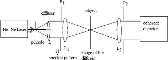
Confocal microscopic imaging of non-scanned object using a diffuser placed in front of the lens L. The two microscope objectives are L1 and L2. The image of the diffuser spreads over the object in its plane

3 Results
The input mammographic image used in the processing is shown in Fig. 2.

We construct random diffuser d (u, v), of dimensions 512 × 512 pixels as shown in Fig. 3. It is placed in front of the collimating lens L. This diffuser incident upon a circular aperture of diameter 128 pixels is given in Fig. 4. The PSF corresponding to the aperture of the collimating lens convoluted with the Fourier spectrum of the diffuser is shown in Fig. 5. It is called modulated speckle pattern since the F.T. of the diffuser is named ordinary speckle assuming high numerical aperture (NA).

A diffuser d (u, v) in the form of randomly distributed function of dimensions 512 × 512 pixels

The diffuser d (u, v) plotted in Fig. 2 obstructed by a circular uniform aperture of radius 128 pixels is shown

The modulated speckle pattern which is the FT of the multiplication of the diffuser and the circular aperture. It is located before the 1st microscope objective
The modulated speckle pattern shown in Fig. 5 is truncated by the 1st microscope objective is shown in Fig. 6.

The modulated speckle pattern shown in Fig. 5 is truncated by the 1st microscope objective. The aperture radius = 128 pixels
The FT of the modulated speckle multiplied by the transmittance from 1st objective of the microscope will give the image of the diffuser convoluted by the PSF of the 1st objective located in the object plane as shown in Fig. 7. The modulus square of the multiplication of the above convolution with the object and the PSF corresponding to the 2nd objective forming the detected noisy image is shown in Fig. 8a. The detected images in absence of the diffuser are shown as in Fig. 8b for aperture radius = 128 pixels, while Fig. 8c shows the image for aperture radius = 16 pixels. The figures from 2 up to 8 represent images of two-dimensional matrix of 512 × 512 pixels starting from (0,0) in the upper left corner and ending with (512, 512) in the lower right corner.

The FT corresponding to the multiplication of the modulated speckle shown and the 1st objective of the microscope shown in Fig. 6. The formed pattern which is the diffuser image convoluted with the PSF corresponding to the 1st objective located in the object plane

a The detected intensity originated from the multiplication of the modulated diffuser with the object transparency affected by the PSF corresponding to both objectives. b The detected intensity obtained in absence of the diffuser using mechanical scanning of the object synchronized with the electronic scanning in the detection plane. The microscope used is called confocal laser scanning microscope (CLSM). The aperture radius = 128 pixels. c The detected intensity obtained in absence of the diffuser. The microscope used is called confocal laser scanning microscope (CLSM). The aperture radius = 16 pixels
4 Discussion
The proposal of NSCM using a diffuser gives reconstructed images in the detection plane affected by the diffuser noise. The reconstructed image may be improved by filtration technique. This new arrangement of NSCM is compared with the ordinary confocal microscope provided with the mechanical scanning of the object placed in the confocal plane of the objectives. It is shown equal resolution in both cases with and without diffuser. The different confocal microscope arrangements gave equal values of resolution since the Resultant Point Spread Function (RPSF) is only dependent on the objectives and the laser beam of wavelength λ. It is computed from the PSF corresponding to each objective lens represented by Eq. (10). The PSF corresponding to uniform circular aperture has the known Airy disc [2].
It is shown a noisy image affected by the diffuser as in Fig. 8a, of resolution dependent on the PSF corresponding to the objectives. The detected intensity for greater radius (128 pixels) shown in Fig. 8b has better resolution than that shown in Fig. 8c for smaller radius = 16 pixels. This is attributed to the inverse relation between resolution and the aperture radius for certain focal length which is determined from the spatial radial cutoff in the focal plane. The PSF using uniform circular aperture versus radial distance in the Fourier plane is plotted as in Fig. 9. The cutoff values computed to represent resolution are as follows:

The PSF using uniform circular aperture of radius = 16 pixels. The cutoff radial distance (rc) = 0.5039 µm as shown in the curve
The cutoff radial distance (rc) = 0.5039 µm for aperture radius = 16 pixels, while (rc) = 0.06 µm for aperture radius = 128 pixels. Another values of cutoff are given as follows: (rc) = 0.2581 µm for aperture radius = 32 pixels, and (rc) = 0.1352 µm for aperture radius = 64 pixels. It is shown inverse relation between the cut-off value rc and the aperture radius as expected from the resolution limit, assuming monochromatic light for the microscope illumination of wavelength λ. The theoretical resolution limit is given by: \({\text{resolution limit = }} \frac{\lambda }{NA}\).
Consequently, the highly resolved images are obtained for sharper PSF hence lower cutoff value as shown in Fig. 8b.
5 Conclusions
A confocal microscope based on substituting the mechanical scanning of the object by the image of the diffuser formed in the object plane. The diffuser is placed before the collimating lens of the spatial filter. Hence, speckle pattern is formed in the back focal plane of the collimating lens which is the Fourier transform of the transmitted diffuser. Then, operating the inverse Fourier transform upon the 1st objective lens limited by the aperture P1 to get the convolution of the diffuser image and the PSF corresponding to the 1st objective. This convolution product is formed in the object plane. Consequently, the detected intensity is computed from the multiplication of the object with the diffuser convoluted with the PSF corresponding to both microscope objectives. The detected image is affected by a noise originated from the diffuser, which can be removed by filtering techniques. Concerning the image resolution using diffuser or in absence of it, we insist upon its dependence upon the aperture radius as outlined in results and discussion.
The potential work of NSCM is to test the confocal microscope, while the object placed in the common short focus of both objectives is fixed and assuming the scanning realized by either diffuser or grating.
Availability of data and materials
Not applicable.
Abbreviations
- NSCM:
-
Non-Scanned Confocal Microscope
- CSLM:
-
Confocal Scanning Laser Microscope
- PSF:
-
Point Spread Function
- RPSF:
-
Resultant Point Spread Function
- ⊗:
-
Symbol for convolution operation
- F.T.:
-
Fourier transform integral and its inverse F.T.−1
- NA:
-
Numerical aperture corresponding to an objective lens
References
Sheppard CJR (1977) The use of lenses with annular aperture in scanning optical microscopy. Optik 48:329–334
Sheppard CJR, Choudhury A (1977) Image formation in the scanning microscope. Opt Acta 24(10):1051–1073
Sheppard CJR, Wilson T (1978) Depth of field in the scanning microscope. Opt Letters 3(3):115–117
Sheppard CJR, Wilson T (1979) Imaging properties of annular lenses. Appl Opt 18(22):3764–3769
Sheppard CJR, Wilson T (1980) Fourier imaging of phase information in conventional and scanning microscopes. Phil Trans R Soc A295:513–536
Cox IJ, Sheppard CJR, Wilson T (1982) Improvement in resolution by nearly confocal microscope. Appl Opt 21(5):778–781
Sheppard CJR, Mao XQ (1988) Confocal microscopes with slit apertures. J Mod Opt 35(7):1169–1185
Sheppard CJR (1988) Super-resolution in confocal imaging. Optik 80(2):53–54
Sheppard CJR, Gu M (1991) Improvement of axial resolution in confocal microscopy using an annular pupil. Opt Commun 84(12):7–13
Sheppard CJR, Gu M (1993) Imaging by a high aperture optical system. J Modern Opt 40(8):1631–1651
Cox G, Sheppard CJR (2004) Practical limits of resolution in confocal and non- linear microscopy. Microsc Res Tech 63(1):18–22
Sheppard CJR, Wilson T (1978) Gaussian beam theory of lenses with annular aperture. IEE J Microw Opt Acoust 2(4):105–112
Clair JJ, Hamed AM (1983) Theoretical studies on optical coherent microscopes. Optik 64(2):133–141
Hamed AM, Clair JJ (1983) Image and super-resolution in optical coherent microscopes. Optik 64(4):277–284
Hamed AM, Clair JJ (1983) Studies on optical properties of confocal scanning optical microscope using pupils with radially transmission ρn distribution. Optik 65(3):209–218
Hamed AM (1984) Opt Laser Technol 16(2):93–96
Hamed AM (2017) Improvement of point spread function (PSF) using linear- quadratic aperture. Optik 131:838–849
Hamed AM (1998) Theoretical study on a coherent non-scanned microscope (CNSM). Optik 107(3):89–92
Hamed AM, Al- Saeed TA (2015) Image analysis of modified Hamming aperture: application on confocal microscopy and holography. J Mod Opt 62(10):801–810
Ragazzi M, Piana S, Longo C et al (2014) Fluorescence confocal microscopy for pathologists. Mod Pathol 27:460–471
Tilly MT, Cabrera MC, Parrish AR et al (2007) Real-time imaging and characterization of human breast tissue by reflectance confocal microscopy. J Biomed Opt 12:051901
Schiff Hauer LM, Boger JN, Buonfiglio TA et al (2009) Confocal microscopy of unfixed breast needle core biopsies: a comparison to fixed and stained sections. BMC Cancer 9:265
Bickford LR, Agollah G, Drezek R, Yu TK (2010) Silica-gold nano shells as potential intraoperative molecular probes for HER2-overexpression in ex vivo breast tissue using near-infrared reflectance confocal microscopy. Breast Cancer Res Treat 120:547–555
Kitabatake S, Niwa Y, Miyahara R et al (2006) Confocal endomicroscopy for the diagnosis of gastric cancer in vivo. Endoscopy 38:1110–1114
Kiesslich R, Goetz M, Burg J et al (2005) Diagnosing helicobacter pylori in vivo by confocal laser endoscopy. Gastroenterology 128:2119–2123
Hamed AM (2019) Design of a cascaded black- linear distribution (CBLD)in circular aperture and its application on confocal laser scanning microscope (CLSM). Am J Opt Photonics 7(3):46–56
Acknowledgements
Not applicable.
Funding
Not applicable.
Author information
Authors and Affiliations
Contributions
The corresponding author, AMH, has presented all steps of the manuscript preparation, including the idea, the method including the theoretical analysis, and the results with discussions. TAA-S has assisted in results and discussions. Both authors read and approved the final manuscript.
Corresponding author
Ethics declarations
Ethics approval and consent to participate
Not applicable.
Consent for publication
Not applicable.
Competing interests
The authors declare that they have no competing interests.
Additional information
Publisher's Note
Springer Nature remains neutral with regard to jurisdictional claims in published maps and institutional affiliations.
Rights and permissions
Open Access This article is licensed under a Creative Commons Attribution 4.0 International License, which permits use, sharing, adaptation, distribution and reproduction in any medium or format, as long as you give appropriate credit to the original author(s) and the source, provide a link to the Creative Commons licence, and indicate if changes were made. The images or other third party material in this article are included in the article's Creative Commons licence, unless indicated otherwise in a credit line to the material. If material is not included in the article's Creative Commons licence and your intended use is not permitted by statutory regulation or exceeds the permitted use, you will need to obtain permission directly from the copyright holder. To view a copy of this licence, visit http://creativecommons.org/licenses/by/4.0/.
About this article

Cite this article
Hamed, A.M., Al-Saeed, T.A. Reconstruction of images in non-scanned confocal microscope (NSCM) using speckle imaging. Beni-Suef Univ J Basic Appl Sci 10, 67 (2021). https://doi.org/10.1186/s43088-021-00157-0
Received:
Accepted:
Published:
DOI: https://doi.org/10.1186/s43088-021-00157-0