
Abstract
Video surveillance systems are essential as other application domain. Handling efficient and reliable for underground projects as well surveillance image is so significant to ensure security and safety. The wireless channels are efficient as data transferring media. On the other hand, the bandwidth may be limited for some environmental conditions. Hence, the image compression algorithm is very important to be conducted and applied to save the transmission bandwidth. This paper presents an image compression algorithm for video surveillance. The method is based on the concept of luminance variation of image. The image compression method is expected to achieve a reasonable compression ratio with acceptable quality. With another meaning, the compressed image size is decreased and consumes a smaller transmission bandwidth via the wireless channel compared with the original image size. The method adopts a deep learning approach to improve the quality with limited bandwidth. The proposed method is abbreviated as DLBL (deep learning block luminance). DLBL implemented and tested on some tested bed images. The performance of the proposed method is compared with some ones considering the same conditions. Some measurable criteria are taken into consideration for performance evaluation. The criteria are the compression ratio (CR), peak signal-to-noise ratio (PSNR) and structure similarity index measure (SSIM). From the experiments results, the proposed method showed significant and efficient performance compared with some other related ones. This is clear from the values of CR, PSNR and SSIM.
Introduction
In recent years, tremendous progress in the sciences of communication and multimedia has been signposted by the widely used monitoring system. Since the monitoring system—video surveillance—is characterized by many advantages such as providing safety for the human and machines, also saving time, effort, and money [1]. Consequently, many projects and applications cannot dispense the video surveillance as an integral part from its systems, such as smart city, smart parking, transport management, and administrative buildings [2, 3]. In particular, underground projects such as engineering construction and exploration have great importance in the economic sector [4, 5]. The nature of underground projects and the surrounding circumstances make the data transmission through the wireless channels is the most appropriate choice, despite the limited bandwidth is used [6]. This situation forced the transmission of data with a limited number of bits, which appears to have a negative impact on the quality of the transmitted data, and it was necessary to minimize this lack of image quality under the available conditions. There upon, several image compression algorithms were introduced to overcome these challenges. Before showing some of these algorithms, it was necessary to explain briefly the general block diagram of the video surveillance systems. Figure 1 illustrates the stages of the video surveillance system, starting with video stream acquisition process using cameras or sensors according to available transmission channels. After that comes one of the top significant steps: stage two, which is video compression. It is controlling the process of reducing the number of bits required to represent a video stream. The output from stage two is becoming ready to transfer through the transmission channels: this is the responsibility https://www.powerthesaurus.org/responsibility/synonyms of the third stage. All required video processing operations such as video recognition and image classification are executed in the fourth stage. If there is any danger, here the role of the fifth and final stage appears by giving a warning [7].

Video surveillance systems block diagram
Now, some previous research efforts are briefly presented [8] suggested an algorithm called denoising-based AMP (D-AMP). It is an extension of the approximate message passing (AMP) framework, depending on the utilization of a suitable Onsager correction in its iterations. Onsager correction converts the signal disturbances at every iteration approximately to the white Gaussian. This is because denoisers are used to manage white Gaussian. Reference [9] described an algorithm exploitation of a classic augmented Lagrangian multiplier approach. In order to limit the use of augmented Lagrangian function at every iteration, it is using an alternating direction algorithm and a nonmonotone line search together. Reference [10] proposed an algorithm aims to reducing the noise effect by utilizing the regularization algorithms: first one is least square QR-factorization, Tikhonov, econdary total variation minimization with augmented Lagrangian, and the last algorithm is alternating direction. Reference [11] explained the DR2-Net algorithm, based on two observations, linear mapping was used to rebuild a preliminary image with good quality, and residual learning makes efficient recovery quality. Reference [12] proposed an image compression method for video surveillance. That method was based on residual network and discrete wavelet transform. The author also presented loss function to train the network. The image compression method presented a reliable compression ratio compared with some other related works. The proposed method concerned both with the structural similarity and peak signal to noise ratio. The proposed method is relevant to be used in the wireless communication environment and it was applied on the underground mines. Reference [13] mentioned that when using wavelet transform, the image is not divided into blocks but processed entirely. This is necessary to eliminate the occurrence of distortions, so images with high compression ratio are not decomposed into blocks but simply lose then clarity due to blurred boarders. The authors in their research work discussed the concept of providing large video compression ratios without deterioration of the image quality. The authors presented a method of brightness processing based on the fixed partitioning of images into blocks. From the experimental work and results, the author method was efficient for processing the video stream.
Reference [14] mentioned that image compression aims mainly at reducing the number of bits required to represent an image both for storage and transmission as well. Machine learning especially deep learning can be utilized to improve the image compression process. Such improvements can take different forms: one of them is removing the quantization coefficients. The authors in their paper presented a short survey paper on image compression process. The paper combined both the traditional compression algorithms and those ones based on deep learning. The authors classified the compression process based on machine learning into several types. Image compression includes, but not limited to, using image features, compression adopting colour images, compression based on the reduction in artifacts, compression based on neural networks, and others.
This work introduces an effective compression method called DLBL based on the variation of the image luminance intensity using deep learning, as will be explained in Section “The Proposed Image Compression method”. The results show that the main objective of the research is achieved by the proposed algorithm, which improves image quality under bandwidth limitation, as shown in “Experiment and results” section.
The rest of this paper is coordinated as follows. Section “Preliminaries” presents some preliminaries. The proposed method is introduced in Section "The Proposed Image Compression method", while “Experiment and results” in section describes the experiments performed using the proposed method and also presents and discusses the experiments results. Finally, “Results and discussion” in section concludes the whole works.
Preliminaries
Residual neural network
One of the most important convolutional neural networks (CNNs) is residual neural network (ResNet). ResNet is a model that is developed in 2016 by He et al. This model is a network that has 50 layers deep. ResNet-50 is an artificial neural network (ANN). This network model is a kind that stacks residual blocks on top of each. 1000 object categories images can be classified by this network. This residual units include convolutional, pooling, activation and fully connected layers and sub-layers. ResNet 50 contains convolutional layers represented in 49 layers and at the last is the fully connected layer. The residual block which is used in this network is shown in Fig. 2. Compared to other networks models. The advantage of the ResNets model is that the performance of this model does not decrease even though the architecture is getting deep [15].

The residual block used in the network
Discrete cosine transform
Discrete cosine transform (DCT) is considered a significant step in image compression algorithms. It is an orthogonal transformation to convert the image for sub-spectral, including two levels of the frequencies: low and high frequency. With other words, DCT changes the image matrix framework from the spatial domain to the frequency domain with the similar size as shown in Fig. 3 using the following Eqs. 1 and 2 [16].
where the input image is represented by a matrix with size N*M. f(i, j) denotes the intensity of a pixel indexed in row i and column j in the matrix for the input image. F(u, v) identifies the coefficient for frequency matrix in row u and column v.

Change the image matrix framework from the spatial domain to the frequency domain using DCT
Low frequency constitutes the energy of the image. That is to say, it contains the most significant information of the image, whereas the high frequency has the remaining of image information [17]. The human eye is perception to low frequency much more the high frequency; therefore, high frequency can be excluded by the use of quantization, as will be clarified later. Thus, a high CR is accomplished [18].
Quantization
The quantization is a process to reduce the quantity values. This reduces the number of bits to be necessary to represent the digital image. The selection of quantization matrices determined the level of quality and CR. In the quantization process, the frequency matrix is divided by the quantization matrix and the result is rounded using Eq. 3. At receiver, the reverse process is done according to Eq. 4, where F(U, V) and Q(U, V) represent the coefficient of frequency and quantization matrixes, respectively [19].
After that, the quantized matrix is converted to a vector, by zigzag method as shown in Fig. 4.

Zigzag scan method
The Proposed Image Compression method
This work presents an effective method to compress an image based on the variation of imageluminance.The block diagram of proposed algorithm is shown in Fig. 5.

Block diagram for proposed method
The method also involves classification using deep learning. It seeks to complete the compression process while preserving the characteristic of the image as possible. The digital image consists of a set of pixels, and each of them has a value of intensity [20]. The DLBL determines the variation of the intensity value between pixels that indicates a change in information of the image. So, DLBL can send only non-duplicate information with perceiving the image characteristic as shown in the following steps:
-
Step 1 The DLBL starts by training a deep learning network using Resent 50 to classify the divided blocks of images to one of three probabilities of illumination intensity: high, medium, and low—offline–and save the trained network to call it in the next steps.
This paper uses Caltech 101 data set “ https://data.caltech.edu/records/20086” to train the ResNet network by preparing the new data set for blocks as given in the following steps:
-
A: Start by dividing data set images to non-overlapping 4*4 blocks
-
B: Calculate the mean of pixels value for each block
-
C: The categorization of blocks based on illumination was done by dividing the range of grey level [0:255] to three uniform parts. The type of block illumination of the mean values [0:84] is considering low, where the mean value between [85:169] is medium and the last if the value between [170:255] is high value.
-
D: The used images are 60,000 and they are divided into 75% for training and 25% for testing.
Figure 6 displays that the trained network achieves high results for validation accuracy arrive to 98.11%.
Fig. 6 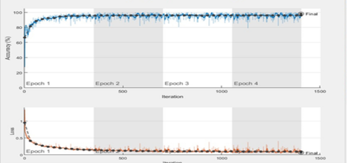
The results of network training processing
-
-
Step 2 DLBL divided the image to non-over lapping blocks with 4 × 4 pixels and analysed the variation in illumination intensity between the current block (CB) and the previous encoded block (PB) using a trained deep learning network from the previous step. Here, there are two possibilities: the first one is the level of luminance intensity for two tested blocks are not identical in this case, DLBL follows the following steps:
-
A: Calculate complementary of CB (CCB) using Eq. 5:
$${\text{CCB}} = 255 - \mathop \sum \limits_{i = 0}^{n} \mathop \sum \limits_{j = 0}^{m} CB\left( {i,j} \right)$$(5) -
B: Calculate the residual between CCB and BP using Eq. 6:
$${\text{Residual}} = \left| {\mathop \sum \limits_{i = 0}^{N} \mathop \sum \limits_{j = 0}^{M} {\text{BP}} - \mathop \sum \limits_{i = 0}^{N} \mathop \sum \limits_{j = 0}^{M} {\text{CCB}} } \right|$$(6) -
The second probability is the two tested blocks are identical; here the residual is calculated directly according to 7:
$${\text{Residual}} = \left| {\mathop \sum \limits_{i = 0}^{N} \mathop \sum \limits_{j = 0}^{M} {\text{BP}} - \mathop \sum \limits_{i = 0}^{N} \mathop \sum \limits_{j = 0}^{M} {\text{CB}} } \right|$$(7)
-
-
Step 3 The obtained residual from step 2 is transformed to the frequency domain using DCT transformation and quantization process as explained in “Residual neural network” and “Discrete cosine transform” this is necessary to encode the output from the previous step. At the decoder, DLBL reverses the previous steps to recover the compressed images.

Experiment and results
The DLBL method is operated and tested using a set of images, until the effectiveness is verified. The experimental results of the proposed algorithms are variously compared with those of the D-AMP [8] algorithm, ReconNet algorithm [21], TVAL3 algorithm [10], DR2-Net algorithm [11], and RNDWT algorithm [12].
Before presenting and discussing the results, a brief description of the database is presented in “Data set description” section. Also, the main criteria to evaluate the performance of the proposed method are presented in “Measurement parameters” section.
Data set description
The data set here is represented as a set of images. These images were collected from various sources: first one—COCO2014 data set, Barbara and fingerprint, as shown in Fig. 7a, b, respectively. The secondary images, video images, were collected from underground projects, coal cutter and tunnel boring machine shown in Fig. 7c and d, respectively [22].

The test images: a Barbara; b fingerprint; c coal cutter; d tunnel boring machine
Measurement parameters
To evaluate quality of recovered images using two image quality matrices: peak-signal-to-noise ratio PSNR and structural similarity index measure (SSIM) [23]. The PSNR is used as a quantitative evaluation, defined by Eq. 8 [24].
where d is the highest scale value of the 8-bits greyscale. The PSNR results from the calculation of the mean square error (MSE) of an image, as defined by Eq. 9 [24].
The MSE approaches zero, and accordingly, PSNR value approaches infinity. Hence, low PSNR means low imagequality which implies high mathematical differences between images, which means reconstructed image have low quality value. On the contrary, a high value of PSNR indicates the presence of low mathematical discrepancies between the images, this indicates the high quality. PSNR is uncomplicated to compute, has clear materialistic meaning, and is mathematical advantageous regarding enhancement. Yet, it experiences an absence of articulation in the visual quality [23, 25].
Whereas SSIM is a good representation for visual quality evaluation, to quantify the closeness between images, SSIM as defined by Eq. 10 depends on three parameters for calculations mainly: loss of correlation, luminance distortion, and contrast distortion as shown in Eqs. 11–13 [26].
I in Eq. 11 is the comparison function, which estimates the level of similarity between the mean luminance \(\left( {\mu_{x} \;{\text{and}}\;\mu_{{\hat{x}}} } \right)\) for two different images. The maximum value of I equals to one at \(\mu_{x} = \mu_{{\hat{x}}}\). Here C is defined by Eq. 12 which is the contrast comparison function. This term measures the closeness of the contrast between the two images by using the standard luminance deviation \(\sigma_{x} \;{\text{and}}\;\sigma_{{\hat{x}}}\). The maximum value of C equals to one if \(\sigma_{x} = \sigma_{{\hat{x}}}\). Last term S in Eq. 13 is indicating the structure comparison function responsible for computing the covariance between the two images x and x^, where \(\sigma_{{x\hat{x}}}\) is the covariance between x and x^. The value of SSIM is between 0 and 1. If SSIM value equals one that means the two images are identical where zero value means no correlation between images. The positive constants C1, C2, and C3 are utilized to prevent an invalid denominator.
Results and discussion
Figures 8, 9, 10, 11, 12, 13, 14, 15 present the results of DLBL and other algorithms: D-AMP, ReconNet, TVAL3, DR2-Net, and RNDWT. The results are for the measurable criteria PSNR and SSIM. at CR of 0.25, 0.20, 0.15, 0.10, 0.04, and 0.01. CR is determined by Eq. 14 [12].
Figures 8, 9, 10, 11 show the quantitative measurement—PSNR—for tested images. DLBL method improves the results at different CR, especially fingerprint, coal cutter, and tunnel boring machine images which are more complicated images; hence, they have more details and edges. Taking into consideration when the CR < 0.1, add Gaussian filter to improve the quality. The results show that with decreasing the CR, the PSNR decreases accordingly, while maintaining the highest results in favour of the DLBL method.

PSNR for barbra

PSNR for fingerprint

PSNR for coal cutter

PSNR for tunnel boring machine

SSIM for Barbara
Figures 11, 12, 13, 14 present the results of the visual quality evaluation SSIM. By the analysis of the figures, it has been observed that the proposed algorithm worked with the same efficiency that prevailed in it, while monitoring the PSNR values in terms of high observed values compared to other algorithms.

SSIM for fingerprint

SSIM for coal cutter

SSIM for tunnel boring machine
From the PSNR and SSIM results that have been monitored. It is noted that DLBL preserves the more features of the images, whereas DLBL depends on sending data has new and significant information for image. This is evident in all tested images, especially the complex images. Finally, the DLBL accomplishes what is required in terms of quality improvement with restricted bandwidth.
Conclusion and future work
In this paper, an image compression method was proposed aims to reduce the number of transmitted bits for compressed image and recover it with high quality specially with images containing many details and sharp edges. The CNN-ResNet50-based image classification algorithm was used to determine the relationship between the image blocks in terms of the change in illumination level to identify the data that contains new information only to be sent. The experimental results establish that the DLBL accomplished a considerable improvement of quality with limited bandwidth. This was achieved for the tested images, yet in addition accomplished a critical improvement in a more complex image. Taking into consideration when the CR ˂ 0.1, add Gaussian filter to improve the quality. From the above, it can be clearly seen that the DLBL is appropriate to compress images and retrieve them in the underground surveillance systems. In future work, the performance of the proposed algorithm can be improved by selecting the hyperparameters of the deep learning model such as batch size, learning rate, and number of hidden layers.
Availability of data and materials
The data sets used and/or analysed during the current study are available from the corresponding author on reasonable request.
References
Gura D, Markovskii I, Khusht N, Rak I, Pshidatok S (2021) A complex for monitoring transport infrastructure facilities based on video surveillance cameras and laser scanners. Transp Res Proc 54:775–782
Jin Y, Qian Z, Yang W (2020) UAV cluster-based video surveillance system optimization in heterogeneous communication of smart cities. IEEE Access 8:55654–55664
Luo H, Liu J, Fang W, Love PED, Yu Q, Lu Z (2020) Real-time smart video surveillance to manage safety: a case study of a transport mega-project. Adv Eng Inform 45:101100
Guo S, Li J, Liang K, Tang B (2021) Improved safety checklist analysis approach using intelligent video surveillance in the construction industry: a case study. Int J Occup Saf Ergon 27(4):1064–1075
Dohare YS, Maity T, Das PS, Paul PS (2015) Wireless communication and environment monitoring in underground coal mines–review. IETE Tech Rev 32(2):140–150
Ma E et al (2021) Review of cutting-edge sensing technologies for urban underground construction. Measurement 167:108289
Wang L et al (2020) Automatic monitoring system in underground engineering construction: review and prospect. Adv Civil Eng 2020:555
Metzler CA, Maleki A, Baraniuk RG (2016) From denoising to compressed sensing. IEEE Trans Inf Theory 62(9):5117–5144
Li C, Yin W, Jiang H, Zhang Y (2013) An efficient augmented Lagrangian method with applications to total variation minimization. Comput Optim Appl 56(3):507–530
Kong Q, Gong R, Liu J, Shao X (2018) Investigation on reconstruction for frequency domain photoacoustic imaging via TVAL3 regularization algorithm. IEEE Photon J 10(5):1–15
Yao H, Dai F, Zhang S, Zhang Y, Tian Q, Xu C (2019) Dr2-net: Deep residual reconstruction network for image compressive sensing. Neurocomputing 359:483–493
Zhang F et al (2019) An image compression method for video surveillance system in underground mines based on residual networks and discrete wavelet transform. Electronics 8(12):1559
Tashmanov EB, Saidboyev BJ, Kamilov MA (2020) Processing of video information in unmanned aerial vehicles. J Crit Rev 7(15):1714–1720
Patel MI, Suthar S, Thakar J (2019) Survey on image compression using machine learning and deep learning. In: IEEE, pp 1103–1105
He K, Zhang X, Ren S, Sun J (2016) Deep residual learning for image recognition, pp 770–778
Hasan TS (2017) Image compression using discrete wavelet transform and discrete cosine transform. J Appl Sci Res 13:1–8
Nageswara RT, Srinivasa KD (2008) Image compression using discrete cosine transform. Comput Sci Telecommun 3:35–44
Tang C-W (2007) Spatiotemporal visual considerations for video coding. IEEE Trans Multimedia 9(2):231–238
Raid AM, Khedr WM, El-Dosuky MA, Ahmed W (2014) Jpeg image compression using discrete cosine transform-a survey. arXiv preprint arXiv:1405.6147
Wang D, Chang C-C, Liu Y, Song G, Liu Y (2015) Digital image scrambling algorithm based on chaotic sequence and decomposition and recombination of pixel values. Int J Netw Secur 17(3):322–327
Kulkarni K, Lohit S, Turaga P, Kerviche R, Ashok A (2016) Reconnet: non-iterative reconstruction of images from compressively sensed measurements, pp 449–458
Lin T-Y et al (2014) Microsoft coco: common objects in context. Springer, Berlin, pp 740–755
Setiadi DRIM (2021) PSNR vs SSIM: imperceptibility quality assessment for image steganography. Multimedia Tools Appl 80(6):8423–8444
Wang Z, Bovik AC (2009) Mean squared error: Love it or leave it? A new look at signal fidelity measures. IEEE Signal Process Mag 26(1):98–117
Hore A, Ziou D (2010) Image quality metrics: PSNR vs. SSIM. In: IEEE, pp 2366–2369
Sara U, Akter M, Uddin MS (2019) Image quality assessment through FSIM, SSIM, MSE and PSNR—a comparative study. J Comput Commun 7(3):8–18
Funding
There has been no significant financial support for this work.
Author information
Authors and Affiliations
Contributions
All the authors listed on the title page have contributed significantly to the work, have read the manuscript, attest to the validity and legitimacy of the data its interpretation and agree to its submission.
Corresponding author
Ethics declarations
Computing interests
The authors declare that they have no computing interests associated with this work.
Additional information
Publisher's Note
Springer Nature remains neutral with regard to jurisdictional claims in published maps and institutional affiliations.
Rights and permissions
Open Access This article is licensed under a Creative Commons Attribution 4.0 International License, which permits use, sharing, adaptation, distribution and reproduction in any medium or format, as long as you give appropriate credit to the original author(s) and the source, provide a link to the Creative Commons licence, and indicate if changes were made. The images or other third party material in this article are included in the article's Creative Commons licence, unless indicated otherwise in a credit line to the material. If material is not included in the article's Creative Commons licence and your intended use is not permitted by statutory regulation or exceeds the permitted use, you will need to obtain permission directly from the copyright holder. To view a copy of this licence, visit http://creativecommons.org/licenses/by/4.0/.
About this article

Cite this article
Khairy, M., Al-Makhlasawy, R.M. A reliable image compression algorithm based on block luminance adopting deep learning for video surveillance application. Journal of Electrical Systems and Inf Technol 9, 21 (2022). https://doi.org/10.1186/s43067-022-00063-0
Received:
Accepted:
Published:
DOI: https://doi.org/10.1186/s43067-022-00063-0