
Abstract
In this paper, we introduce the notion of an α–ζ̃– –Pata contraction that combines well-known concepts, such as the Pata contraction, the E-contraction and the simulation function. Existence and uniqueness of a fixed point of such mappings are investigated in the setting of a complete metric space. An example is stated to indicate the validity of the observed result. At the end, we give an application on the solution of nonlinear fractional differential equations.
1 Introduction
In 2015, Khojasteh et al. [1] initiated the concept of simulation functions.
Definition 1.1
([1])
A mapping \(\zeta :[0,\infty )\times {}[ 0,\infty )\rightarrow \mathbb{R}\) is called a simulation function if the following conditions hold:
- \((\zeta _{1})\):
-
 for all
  ;
; - \((\zeta _{2})\):
-
if
 ,
,  are sequences in \((0,\infty )\) such that
  , then
 (1.1)
(1.1)
 for all
  ;
; ,
,  are sequences in
  , then

We denote by \(\mathcal{Z}\) the family of all above simulation functions.
Let  be a metric space and \(\alpha :\mathcal{X}\times \mathcal{X}\rightarrow [0,\infty )\) be a function. A mapping
  is called α-orbital admissible if the following condition holds:

for all \(\nu \in \mathcal{X}\). Moreover, an α-orbital admissible mapping is called triangular α-orbital admissible if for all \(\nu , \omega \in \mathcal{X}\), we have

Definition 1.2
A set \(\mathcal{X}\) is said to be regular with respect to a given function \(\alpha :\mathcal{X}\times \mathcal{X} \to [0,\infty )\) if for each sequence \(\{\nu _{n}\}\) in \(\mathcal{X}\) such that \(\alpha (\nu _{n},\nu _{n+1})\geq 1\) for all n and \(\nu _{n} \rightarrow \nu \in \mathcal{X}\) as \(n\rightarrow \infty \), then \(\alpha (\nu _{n},\nu )\geq 1\) for all n.
The notion of α-admissible \(\mathcal{Z}\)-contractions with respect to a given simulation function was merged and used by Karapinar in [2]. Using this new type of contractive mappings, he investigated the existence and uniqueness of a fixed point in standard metric spaces.
Definition 1.3
([2])
Let T be a self-mapping defined on a metric space \((\mathcal{X}, d)\). If there exist a function \(\zeta \in \mathcal{Z}\) and \(\alpha :\mathcal{X}\times \mathcal{X} \to [0,\infty )\) such that
then we say that T is an α-admissible \(\mathcal{Z}\)-contraction with respect to ζ.
Theorem 1.4
([2])
Let \((\mathcal{X},d)\)be a complete metric space and let \(T:\mathcal{X}\rightarrow \mathcal{X}\)be an α-admissible \(\mathcal{Z}\)-contraction with respect to ζ. Suppose that:
-
(a)
T is triangular α-orbital admissible;
-
(b)
there exists \(\nu _{0}\in \mathcal{X}\)such that \(\alpha (\nu _{0}, T\nu _{0})\geq 1\);
-
(c)
T is continuous.
Then there is \(\nu _{*}\in \mathcal{X}\)such that \(T\nu _{*}=\nu _{*}\).
Remark 1.5
The continuity condition in Theorem 1.4 can be replaced by the “regularity” condition, which is considered in Definition 1.2.
We will consider the following set of functions:

and we denote

Several interesting extensions and generalizations of the Banach contraction principle [3] appeared in the literature. For instance, see [4–10]. Among these generalizations, we cite the paper of Pata [11]. Since then, much work appeared in the same direction; see [12–15].
Theorem 1.6
([11])
Let  be a complete metric space and let \(\Lambda \geq 0\), \(\lambda \geq 1\), \(\beta \in [0,\lambda ]\)be fixed constants. The mapping
  has a fixed point in \(\mathcal{X}\)if the inequality

is satisfied for every \(\varepsilon \in [0,1]\)and  .
.
Definition 1.7
Let  be a metric space. We say that
  is a Pata type Zamfirescu mapping if for all \(\nu , \omega \in \mathcal{X}\), \(\psi \in \mathcal{Z}\) and for every \(\varepsilon \in [0,1]\),
  , it satisfies the following inequality:

where

and \(\Lambda \geq 0\), \(\lambda \geq 1\) and \(\beta \in [0,\lambda ]\) are constants.
Theorem 1.8
([16])
Let  be a complete metric space and let
  be a Pata type Zamfirescu mapping. Then
  has a unique fixed point in \(\mathcal{X}\).
We state the following useful known lemma.
Lemma 1.9
Let  be a complete metric space and
  be a sequence in \(\mathcal{X}\)such that
  . If the sequence
  is not Cauchy, then there exist
  and subsequences
  and
and  of
of  such that

and

In this paper, we combine the concepts of simulation functions and α-admissibility to give a generalized Pata type fixed point result. At the end, we present an application on fractional calculus.
2 Main results
We denote by \(\tilde{\mathcal{Z}}\) the set of all functions \(\tilde{\zeta }:[0,\infty )\times {}[ 0,\infty )\rightarrow \mathbb{R}\) satisfying the following condition:
- \((\tilde{\zeta }_{1})\):
-
 for all
  .
.
 for all
  .
.Definition 2.1
Let  be a metric space and \(\phi \in \Phi \). Let \(\Lambda \geq 0\), \(\lambda \geq 1\) and \(\beta \in [0,\lambda ]\) be fixed constants. A triangular α-orbital admissible mapping
  is called an α-ζ̃-
 - Pata contraction if there exists a function \(\tilde{\zeta }\in \tilde{\mathcal{Z}}\) such that, for every \(\varepsilon \in [0,1]\), the following condition is satisfied:

for all \(\nu ,\omega \in \mathcal{X}\), where

and

Remark 2.2
It is clear that any Pata type Zamfirescu mapping is also an α-ζ̃- - Pata mapping. Indeed, letting \(\alpha (\nu , \omega )=1\) and
  , the inequality (2.1) becomes

Moreover, note that  for all \(\nu , \omega \in \mathcal{X}\).
Theorem 2.3
Every α–ζ̃– –Pata contraction
  on a complete metric space
  possesses a fixed point if
- (i):
-
there exists
 such that
  ;
; - (ii):
-
 is triangular α-orbital admissible;
 - (iii):
-
either
 is continuous, or the set \(\mathcal{X}\)is regular.
 such that
  ;
; is triangular α-orbital admissible;
 is continuous, or the set
 If in addition we assume that the following condition is satisfied:
- (iv):
-
 for all
  ,
,
 for all
  ,
,then such a fixed point of  is unique.
Proof
Let  be a point such that
  . On account of the assumption that
  is a triangular α-orbital admissible mapping, we derive that

and iteratively we find

Moreover, by (2.4) together with (1.3), we have

Again, iteratively, one writes

Starting from this point  , we build an iterative sequence
  where
where  for \(n=1,2,3, \ldots \). We can presume that any two consequent terms of this sequence are distinct. Indeed, if, on the contrary, there exists \(i_{0} \in \mathbb{N}\) such that

then  is a fixed point. To avoid this, we will assume in the following that for all \(n\in \mathbb{N}\)

We mention that (2.4) can be rewritten as

respectively,

for any \(n \in \mathbb{N}\). In the sequel, we will denote  for all \(\nu \in X\).
Since  is an α-ζ̃-
 -Pata contraction, we have

Thus, taking into account \((\tilde{\zeta }_{1})\), together with (2.6) we get

where

and

Denoting by  , we have

Thus, (2.8) becomes

We claim that the sequence \(\{ \gamma _{n} \} \) is non-increasing. Indeed, if we suppose the contrary that, for some p, \(\gamma _{p}<\gamma _{p+1}\), and so \(\max \{ \gamma _{p}, \gamma _{p+1} \} =\gamma _{p+1}\), then we have \(\vert \gamma _{p}-\gamma _{p+1} \vert =\gamma _{p+1}-\gamma _{p}\).

Consequently, from (2.9), we get, for such an integer p,

The above inequality is true for all \(\varepsilon \in [0,1]\). In particular, for \(\varepsilon =0\), we get \(\gamma _{p+1}\leq \gamma _{p+1}\), which clearly is a contradiction. In this case, we find that the sequence \(\{ \gamma _{n} \} \) is non-increasing. So we can find a non-negative real number γ such that

We claim that \(\gamma =0\). In order to prove this, we have to show that the sequence \(\{ \kappa _{n} \} \) is bounded, where  . Since the sequence
  is non-increasing, we have

By the triangle inequality, we get

On account of (2.5), regarding that  is an α-ζ̃-Pata-
 contraction, we have

Taking into account (2.7), this is equivalent to

Using (2.12) and the above inequality, we get

Moreover, since \(\beta \leq \lambda \), we have
Now, supposing that the sequence \(\{ \kappa _{n} \} \) is not bounded, there exists a subsequence \(\{ \kappa _{n_{l}} \} \) of \(\{ \kappa _{n} \} \) such that \(\kappa _{n_{l}}\rightarrow \infty \) as \(l\rightarrow \infty \). In this case, letting \(\varepsilon =\varepsilon _{l}=\frac{1+3\kappa _{1}}{\kappa _{n_{l}}} ( \in [0,1])\), the above inequality yields
This is a contradiction. Thus, we conclude that our presumption is false and then the sequence \(\{ \kappa _{n} \} \) is bounded. Furthermore, there exists  such that
  for all \(n\in \mathbb{N}\).
Let us go back now and prove that \(\gamma =0\) (where \(\gamma =\lim_{n\rightarrow \infty }\gamma _{n}\)). In view of (2.10) and the fact that the sequence \(\{ \gamma _{n} \} \) is non-increasing, one writes

Recall that

Taking into account that  is an α-ζ̃-\({E_{*}}\) contraction, keeping in mind (2.6) and using \((\tilde{\zeta }_{1})\), we have

We have

Letting \(n \to \infty \) in the previous inequality, we obtain

which is equivalent to

When \(\varepsilon \rightarrow 0\), we get \(\gamma \leq 0\). Therefore,

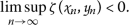
As a next step, we claim that  is a Cauchy sequence. On the contrary, assuming that the sequence is not Cauchy, it follows from Lemma 1.9 that there exist
  and subsequences
  and
and  such that (1.7) and (1.8) hold. Replacing
  and
and  in (2.1), we have

where

The triangular α-orbital admissibility of  shows that
  . Thus,

Letting \(l\rightarrow \infty \) and taking into account (2.14) and Lemma 1.9, we have

At the same time, one writes

Denoting by  and
and  , by Lemma 1.9, it follows that

Thus, passing to the limit as \(l\rightarrow \infty \) in (2.16), we get

Furthermore,

i.e.,

That is,  . Therefore,
  is a Cauchy sequence in the complete metric space. For this reason, there exists \(\nu ^{*}\in \mathcal{X}\) such that
  , as \(n\rightarrow \infty \).
Furthermore, in the case that  is a continuous mapping, we get
  , that is,
  is a fixed point of
  .
.
Now, suppose that \(\mathcal{X}\) is regular. From (2.1), one writes

Using the regularity of \(\mathcal{X}\) and \((\tilde{\zeta }_{1})\), we get

where

and

Taking into account the boundedness of the sequence \(\{ \kappa _{n} \} \), we have

On the other hand,

Letting \(n\rightarrow \infty \) in the inequality (2.19), we find

which is equivalent to

Obviously, we obtain for \(\varepsilon =0\) that  , so
, so  . Thus, \(\nu ^{*}\) is a fixed point of
  . Finally, to prove the uniqueness of the fixed point, we suppose that there exist two fixed points
  such that \(\nu ^{*}\neq \omega ^{*}\). We have

Taking into account \((\mathit{iv})\), we obtain

which leads to

In the limit \(\varepsilon \rightarrow 0\), we get  , that is, \(\nu ^{*}=\omega ^{*}\), which is a contradiction. Therefore, the fixed point of
  is unique. □
In the following, we present an example that supports our statement, that is, Theorem 2.3 is a generalization of Theorem 1.8.
Example 2.4
Take \(\mathcal{X}=A \times A\), where \(A=[0,11]\) and  is the usual distance. Define the mapping
  by
by

where  . For \(\nu _{1}=(11,0)\) and \(\nu _{2}=(2,0)\), we have

and

Thus,

so that the inequality (1.6) does not hold for \(\varepsilon =0\). That is,  is not a Pata type Zamfirescu mapping.
Consider the function \(\alpha :\mathcal{X}\times \mathcal{X} \to [0,\infty )\) given as
Since the assumptions \((i)\)–\((\mathit{iv})\) are obviously satisfied, we have to prove that  is an α-ζ̃-
 - Pata contraction. Take \(\alpha =\beta =1\), \(\Lambda =6\) and the functions \(\Psi (t)=\frac{t}{2}\),
  .
.
For \(\nu , \omega \in B\), we have  , so that (2.1) holds.
For \(\nu =(11,0)\) and \(\omega =(2,0)\) we have

Due to the way the function α was defined, we omit the other cases.
3 An application on a fractional boundary value problem
In this section, we ensure the existence of a solution of a nonlinear fractional differential equation (for more related details, see [17–23]). Denote by \(\mathcal{X}= C[0,1]\) the set of all continuous functions defined on \([0,1]\). We endow \(\mathcal{X}\) with the metric given as
Consider the fractional differential equation
with boundary conditions
Here, \({}^{c}D^{\mu }\) corresponds for the Caputo fractional derivative of order μ, given as
where \(n-1<\mu <n\) and \(n=[\mu ]+1\), and \(I^{\mu }f\) is the Riemann–Liouville fractional integral of order μ of a continuous function f, defined by
In [24], it is showed that the problem (3.1) and (3.2) can be written in the following integral form:
Theorem 3.1
Assume that
-
1.
\(f:[0,1]\times \mathbb{R}\rightarrow \mathbb{R}\)is continuous;
-
2.
for all \(\rho ,\omega \in \mathcal{X}\), we have
$$ \bigl\vert f\bigl(s,\rho (s)\bigr)-f\bigl(s,\omega (s)\bigr) \bigr\vert \leq \frac{\varepsilon ^{2}}{4}\Gamma ( \mu +1) \bigl\vert \rho (s)-\omega (s) \bigr\vert , $$(3.6)for each \(s\in [0,1]\), where \(\varepsilon \in [0,1]\).
Then the problem 3.1and 3.2possesses a unique solution.
Proof
Consider the functional
Note that a solution of (3.5) is also a fixed point of T. We mention that T is well posed. For all \(\rho ,\omega \in \mathcal{X}\) and \(s\in [0,1]\), we have
where B is the beta function. Consequently, one has

where \(\psi (\varepsilon )=\varepsilon \), \(\beta =\lambda =1\) and \(\Lambda =2\). Applying Theorem 2.3, the functional T admits a unique fixed point, that is, the problem (3.1) and (3.2) possesses a unique solution. □
4 Conclusion and remarks
Our results merged from and generalized several existing results in the related literature. First of all, as underlined in Remark 2.2, the main result of [16] is a consequence of our given theorem. On the other hand, by choosing the auxiliary functions in a proper way, we may state a long list of corollaries. More precisely, by choosing the mapping α in a proper way, we can get the analogue of our result in the setting of partially ordered metric spaces, or in the set-up of cyclic mappings. Note that, if we take \(\alpha (x,y)=1\) for all x, y, we get the standard fixed point theorems in the context of complete metric spaces; see [25–29]. In addition, by choosing the appropriate simulation function, one can get several more results; see [30–35].
References
Khojasteh, F., Shukla, S., Radenović, S.: A new approach to the study of fixed point theorems via simulation functions. Filomat 29(6), 1189–1194 (2015)
Karapınar, E.: Fixed points results via simulation functions. Filomat 30, 2343–2350 (2016)
Banach, S.: Sur les opérations dans les ensembles abstraits et leur application aux équations intégrales. Fundam. Math. 3, 133–181 (1922)
Agarwal, P., Jleli, M., Samet, B.: A coupled fixed point problem under a finite number of equality constraints. In: Fixed Point Theory in Metric Spaces, pp. 123–138. Springer, Singapore (2018)
Abdeljawad, T., Mlaiki, N., Aydi, H., Souayah, N.: Double controlled metric type spaces and some fixed point results. Mathematics 6(12), 320 (2018)
Agarwal, P., Jleli, M., Samet, B.: JS-metric spaces and fixed point results. In: Fixed Point Theory in Metric Spaces, pp. 139–153. Springer, Singapore (2018)
Alamgir, N., Kiran, Q., Isık, H., Aydi, H.: Fixed point results via a Hausdorff controlled type metric. Adv. Differ. Equ. 2020, 24 (2020)
Afshari, H., Aydi, H., Karapınar, E.: On generalized \(\alpha -\psi \)-Geraghty contractions on b-metric spaces. Georgian Math. J. 27(1), 9–21 (2020)
Agarwal, P., Jleli, M., Samet, B.: On Ran–Reurings fixed point theorem. In: Fixed Point Theory in Metric Spaces, pp. 25–44. Springer, Singapore (2018)
Asim, M., Nisar, K.S., Morsy, A., Imdad, M.: Extended rectangular \(M_{r\xi }\)-metric spaces and fixed point results. Mathematics 7(12), 1136 (2019)
Pata, V.: A fixed point theorem in metric spaces. J. Fixed Point Theory Appl. 10, 299–305 (2011)
Kadelburg, Z., Radenović, S.: Fixed point theorems under Pata-type conditions in metric spaces. J. Egypt. Math. Soc. 24, 77–82 (2016)
Kadelburg, Z., Radenović, S.: A note on Pata-type cyclic contractions. Sarajevo J. Math. 11(24), No. 2, 235–245 (2015)
Kadelburg, Z., Radenović, S.: Pata-type common fixed point results in b-metric and b-rectangular metric spaces. J. Nonlinear Sci. Appl. 8, 944–954 (2015)
Kadelburg, Z., Radenović, S.: Fixed point and tripled fixed point theprems under Pata-type conditions in ordered metric spaces. Int. J. Anal. Appl. 6(1), 113–122 (2014)
Jacob, G.K., Khan, M.S., Park, C., Yun, S.: On generalized Pata type contractions. Mathematics 6, 25 (2018)
Valliammal, N., Ravichandran, C., Nisar, K.S.: Solutions to fractional neutral delay differential nonlocal systems. Chaos Solitons Fractals 138, 109912 (2020)
Aydi, H., Jleli, M., Samet, B.: On positive solutions for a fractional thermostat model with a convex–concave source term via ψ-Caputo fractional derivative. Mediterr. J. Math. 17(1), 16 (2020)
Shaikh, A.S., Nisar, K.S.: Transmission dynamics of fractional order Typhoid fever model using Caputo–Fabrizio operator. Chaos Solitons Fractals 128, 355–365 (2019)
Budhia, L., Aydi, H., Ansari, A.H., Gopal, D.: Some new fixed point results in rectangular metric spaces with an application to fractional-order functional differential equations. Nonlinear Anal., Model. Control 25, 1–18 (2020)
Ameer, E., Aydi, H., Arshad, M., De la Sen, M.: Hybrid Ćirić type graphic \(( \Upsilon ,\Lambda ) \)-contraction mappings with applications to electric circuit and fractional differential equations. Symmetry 12(3), 467 (2020)
Shaikh, A., Tassaddiq, A., Nisar, K.S., Baleanu, D.: Analysis of differential equations involving Caputo–Fabrizio fractional operator and its applications to reaction diffusion equations. Adv. Differ. Equ. 2019, 178 (2019)
Shatanawi, W., Karapinar, E., Aydi, H., Fulga, A.: Wardowski type contractions with applications on Caputo type nonlinear fractional differential equations. Sci. Bull. “Politeh.” Univ. Buchar., Ser. A, Appl. Math. Phys. 82(2), 157–170 (2020)
Senapati, T., Dey, L.K.: Relation-theoretic metrical fixed point results via w-distance with applications. J. Fixed Point Theory Appl. 19(4), 2945–2961 (2017)
Karapinar, E., Samet, B.: Generalized \((\alpha -\psi )\) contractive type mappings and related fixed point theorems with applications. Abstr. Appl. Anal. 2012, Article ID 793486 (2012)
Alsulami, H., Gulyaz, S., Karapinar, E., Erhan, I.M.: Fixed point theorems for a class of alpha-admissible contractions and applications to boundary value problem. Abstr. Appl. Anal. 2014, Article ID 187031 (2014)
Aksoy, U., Karapinar, E., Erhan, I.M.: Fixed points of generalized α-admissible contractions on b-metric spaces with an application to boundary value problems. J. Nonlinear Convex Anal. 17(6), 1095–1108 (2016)
Ameer, E., Aydi, H., Arshad, M., Alsamir, H., Noorani, M.S.: Hybrid multivalued type contraction mappings in \(\alpha _{K}\)-complete partial b-metric spaces and applications. Symmetry 11(1), 86 (2019)
Aydi, H., Karapinar, E., Francisco Roldan Lopez de Hierro, A.: w-interpolative Ciric–Reich–Rus type contractions. Mathematics 7(1), 57 (2019)
Alghamdi, M.A., Gulyaz-Ozyurt, S., Karapınar, E.: A note on extended Z-contraction. Mathematics 8, 195 (2020)
Agarwal, R.P., Karapinar, E.: Interpolative Rus–Reich–Ciric type contractions via simulation functions. An. Ştiinţ. Univ. ‘Ovidius’ Constanţa, Ser. Mat. 27(3), 137–152 (2019)
Alqahtani, O., Karapinar, E.: A bilateral contraction via simulation function. Filomat 33(15), 4837–4843 (2019)
Aydi, H., Lakzian, H., Mitrovic, Z.D., Radenovic, S.: Best proximity points of MF-cyclic contractions with property UC. Numer. Funct. Anal. Optim. 41(7), 871–882 (2020)
Ma, Z., Asif, A., Aydi, H., Ullah Khan, S., Arshad, M.: Analysis of F-contractions in function weighted metric spaces with an application. Open Math. 18, 582–594 (2020)
Roldan Lopez de Hierro, A.F., Karapınar, E., Roldan Lopez de Hierro, C., Martinez-Moreno, J.: Coincidence point theorems on metric spaces via simulation functions. J. Comput. Appl. Math. 275, 345–355 (2015)
Acknowledgements
The authors thank the anonymous referees for their remarkable comments, suggestions, and ideas, which helped to improve this paper. The authors also thanks to their universities.
Availability of data and materials
No data were used to support this study. It is not applicable for our paper.
Funding
We declare that funding is not applicable for our paper.
Author information
Authors and Affiliations
Contributions
Writing-review and editing were done by HA, AF and EK. All authors contributed equally and significantly in writing this article. All authors have read and agreed to the published version of the manuscript.
Corresponding author
Ethics declarations
Competing interests
The authors declare that they have no competing interests.
Rights and permissions
Open Access This article is licensed under a Creative Commons Attribution 4.0 International License, which permits use, sharing, adaptation, distribution and reproduction in any medium or format, as long as you give appropriate credit to the original author(s) and the source, provide a link to the Creative Commons licence, and indicate if changes were made. The images or other third party material in this article are included in the article’s Creative Commons licence, unless indicated otherwise in a credit line to the material. If material is not included in the article’s Creative Commons licence and your intended use is not permitted by statutory regulation or exceeds the permitted use, you will need to obtain permission directly from the copyright holder. To view a copy of this licence, visit http://creativecommons.org/licenses/by/4.0/.
About this article

Cite this article
Karapinar, E., Fulga, A. & Aydi, H. Study on Pata E-contractions. Adv Differ Equ 2020, 539 (2020). https://doi.org/10.1186/s13662-020-02992-4
Received:
Accepted:
Published:
DOI: https://doi.org/10.1186/s13662-020-02992-4