
Abstract
A non-selective harvesting Lotka–Volterra amensalism model incorporating partial closure for the populations is proposed and studied in this paper. Local and global stability of the boundary and interior equilibria are investigated. By introducing the harvesting, the dynamic behaviors of the system become complicated. Depending on the fraction of the stock available for harvesting, the system maybe extinction, partial survival or two species may coexist in a stable state. Our results supplement and complement the main results of Xiong, Wang, and Zhang (Adv. Appl. Math. 5(2):255-261, 2016).
1 Introduction
Amensalism is one of the basic interactions between the species, where a species inflicts harm on the other species without any costs or benefits received by the other. During the last decade, many scholars [1–15] investigated the dynamic behaviors of the amensalism model. Such topics as the local stability of the equilibrium [1, 5, 12, 14], the existence of the positive periodic solution [2, 11, 13], extinction of the species [3], bifurcation of the system with delay [7] and the influence of the refuge [10, 14] have been studied and many excellent results have been obtained. Recently, Xiong et al. [1] proposed the following amensalism model:
where \(r_{i}, P_{i}, u, i=1, 2\), are all positive constants. The system admits four equilibria:
Concerned with the stability property of the above equilibria, the authors obtained the following results.
Theorem A
-
(1)
\(A(0,0)\) is unstable;
-
(2)
\(B(P_{1}, 0) \) is a saddle point, thus is unstable;
-
(3)
if \(u<\frac{P_{1}}{P_{2}}\), \(C(0, P_{2})\) is a saddle point and consequently unstable; if \(u>\frac{P_{1}}{P_{2}}\), \(C(0, P_{2})\) is a stable node;
-
(4)
if \(u<\frac{P_{1}}{P_{2}}\), \(D(P_{1}-uP_{2}, P_{2})\) is a stable node.
On the other hand, as was pointed out by Chakraborty et al. [16], the study of resource management, including fisheries, forestry, and wildlife management, has great importance. They argued that it is necessary to harvest the population, but harvesting should be regulated so that both the ecological sustainability and conservation of the species can be implemented in a long run. Already, they proposed a non-selective harvesting predator–prey system incorporating partial closure for the populations, they investigated the local and global stability property of the system, and some interesting results related to the optimal harvesting were obtained.
Though there are many papers concerned with the harvesting of the ecosystem system [15–26], to this day, seldom did scholars consider the influence of harvesting on the amensalism model. Stimulated by the works of Xiong et al. [1] and Chakraborty et al. [16], in this paper, we propose the following non-selective harvesting Lotka–Volterra amensalism model incorporating partial closure for the populations:
where \(r_{i}\), \(P_{i}\), u, \(i=1, 2\), are all positive constants. \(r_{i}(P_{i})\) represents the intrinsic growth rate (environmental carrying capacity) of the ith species, E is the combined fishing effort used to harvest and \(m(0< m<1)\) is the fraction of the stock available for harvesting. One could refer to [1, 16] for more background and the adjustment of system (1.2).
As far as system (1.2) is concerned, one interesting issue is the following:
Find out the influence of the parameter m, which reflects the fraction of the stock available for harvesting.
The paper is arranged as follows. We investigate the existence and locally stability property of the equilibrium solutions of system (1.2) in the next section. In Sect. 3, by constructing some suitable Lyapunov function, we investigate the global stability property of the equilibria. The influence of the parameter m is then discussed in Sect. 4. Some examples together with their numeric simulations are presented in Sect. 5 to show the feasibility of the main results. We end this paper with a brief discussion.
2 Local stability of the equilibria
The system always admits the boundary equilibrium \(A(0,0)\).
If \(r_{1}>Emq_{1}\) holds, the system admits the boundary equilibrium \(B(N_{10}, 0)\), where \(N_{10}= \frac{P_{1}(r_{1}-Emq _{1})}{r_{1}}\).
If \(r_{2}>Emq_{2}\) holds, the system admits the boundary equilibrium \(C(0, N_{20})\), where \(N_{20}= \frac{P_{2}(r_{2}-Emq _{2})}{r_{2}}\).
If \(r_{1}r_{2}P_{1}+r_{1}umEP_{2}q_{2}>r_{1}r_{2}uP_{2}+r_{2}mq _{1}EP_{1}\) and \(r_{2}>Emq_{2}\) hold, then the system admits a unique positive equilibrium
We shall now investigate the local stability property of the above equilibria.
The variational matrix of the system of Eq. (1.2) is
where
Theorem 2.1
-
(1)
Assume that
$$ m>\max \biggl\{ \frac{r_{1}}{Eq_{1}}, \frac{r_{2}}{Eq_{2}} \biggr\} $$(2.2)holds, then \(A(0,0)\) is locally stable, otherwise it is unstable;
-
(2)
Assume that
$$ \frac{r_{2}}{Eq_{2}}< m< \frac{r_{1}}{Eq_{1}} $$(2.3)holds, then \(B(N_{10}, 0)\) is locally stable, otherwise it is unstable;
-
(3)
Assume that
$$ \frac{r_{1}r_{2}(P_{1}-uP_{2})}{r_{2}q_{1}EP_{1}- r_{1}uEP_{2}q _{2}} < m< \frac{r_{2}}{Eq_{2}} $$(2.4)holds, then \(C(0, N_{20})\) is locally stable, otherwise it is unstable;
-
(4)
Assume that
$$ m< \min \biggl\{ \frac{r_{2}}{Eq_{2}}, \frac{r_{1}r_{2}(P_{1}-uP_{2})}{r _{2}q_{1}EP_{1}- r_{1}uEP_{2}q_{2}} \biggr\} $$(2.5)holds, then \(D(N_{1}^{*}, N_{2}^{*})\) is locally stable.
Proof
(1) From (2.1) we could see that the Jacobian of the system about the equilibrium point \(A(0,0)\) is given by
The eigenvalues of the matrix are \(\lambda_{1}=r_{1}-Emq_{1}, \lambda _{2}=r_{2}-Emq_{2}\). Hence, under assumption (2.2), \(\lambda_{1}<0, \lambda_{2}<0\), and \(A(0,0)\) is locally stable, otherwise it is unstable;
(2) The Jacobian of the system about the equilibrium point \(B(N_{10},0)\) is given by
The eigenvalues of the matrix are \(\lambda_{1}=Emq_{1}-r_{1}, \lambda _{2}= r_{2}-Emq_{2}\). Under assumption (2.3), \(\lambda_{1}<0, \lambda _{2}<0\), and \(B(N_{10}, 0)\) is locally stable, otherwise it is unstable;
(3) The Jacobian of the system about the equilibrium point \(C(0,N_{20})\) is given by
Under assumption (2.4), the two eigenvalues of the matrix satisfy
Consequently, \(C(0, N_{20})\) is locally stable, otherwise it is unstable;
(4) Noting that the positive equilibrium \(D(N_{1}^{*}, N_{2}^{*})\) satisfies
combining with (2.1) and (2.9), we could see that the Jacobian of the system about the equilibrium point \(D(N_{1}^{*},N_{2}^{*})\) is given by
The eigenvalues of the variational matrix (2.10) are the roots \(\lambda_{1}=- \frac{r_{1}N_{1}^{*}}{P_{1}}<0, \lambda_{2}=- \frac{r _{2}N_{2}^{*}}{P_{2}}<0\). Thus, \(D(N_{1}^{*}, N_{2}^{*})\) is locally stable.
The proof of Theorem 2.1 is finished. □
3 Global stability
One interesting problem is to further investigate the global stability property of the equilibria of system (1.2), since the global one means that despite the random initial condition, the finial dynamic behaviors of the system could be forecasted. In this aspect, we could obtain the following result.
Theorem 3.1
-
(1)
Assume that
$$ m>\max \biggl\{ \frac{r_{1}}{Eq_{1}}, \frac{r_{2}}{Eq_{2}} \biggr\} $$(3.1)holds, then \(A(0,0)\) is globally asymptotically stable;
-
(2)
Assume that
$$ \frac{r_{2}}{Eq_{2}}< m< \frac{r_{1}}{Eq_{1}} $$(3.2)holds, then \(B(N_{10}, 0)\) is globally asymptotically stable;
-
(3)
Assume that
$$ \frac{r_{2}}{Eq_{2}}>m> \frac{r_{1}}{Eq_{1}} $$(3.3)holds, then \(C(0, N_{20})\) is globally asymptotically stable;
-
(4)
Assume that
$$ m< \min \biggl\{ \frac{r_{2}}{Eq_{2}}, \frac{r_{1}r_{2}(P_{1}-uP_{2})}{r _{2}q_{1}EP_{1}- r_{1}uEP_{2}q_{2}} \biggr\} $$(3.4)holds, then \(D(N_{1}^{*}, N_{2}^{*})\) is globally asymptotically stable.
Proof
We will prove Theorem 3.1 by constructing some suitable Lyapunov functions.
(1) We define a Lyapunov function
One could easily see that the function \(V_{1}\) is zero at the equilibrium \(A(0,0)\) and is positive for all other positive values of \(N_{1}\) and \(N_{2}\). The time derivative of \(V_{1}\) along the trajectories of (1.2) is
Obviously, under assumption (3.1), \(D^{+}V_{1}(t)<0\) strictly for all \(N_{1}, N_{2}>0\) except the boundary equilibrium \(A(0, 0)\), where \(D^{+}V_{1}(t)=0\). Thus, \(V_{1}(N_{1},N_{2})\) satisfies Lyapunov’s asymptotic stability theorem, and the boundary equilibrium \(A(0, 0)\) of system (1.2) is globally asymptotically stable.
(2) Noting that \((N_{10},0)\) satisfies
we define a Lyapunov function
where η is a suitable constant to be determined in the subsequent steps. One could easily see that the function \(V_{2}\) is zero at the equilibrium \(B(N_{10},0)\) and is positive for all other positive values of \(N_{1}\) and \(N_{2}\). By applying (3.6), the time derivative of \(V_{2}\) along the trajectories of (1.2) is
Noting that \(r_{2}< Emq_{2}\), we can choose \(\eta = \frac{( Eq_{2}m-r _{2})P_{1}}{N_{10}r_{1}u}>0\), and
Therefore, \(D^{+}V_{2}(t)<0\) strictly for all \(N_{1}, N_{2}>0\) except the boundary equilibrium \(B(N_{10}, 0)\), where \(D^{+}V_{2}(t)=0\). Thus, \(V_{2}(N_{1},N_{2})\) satisfies Lyapunov’s asymptotic stability theorem, and the boundary equilibrium \(B(N_{10}, 0)\) of system (1.2) is globally asymptotically stable.
(3) Noting that \(C(0,N_{20})\) satisfies
we define a Lyapunov function
One could easily see that the function \(V_{3}\) is zero at the equilibrium \(C(0,N_{20})\) and is positive for all other positive values of \(N_{1}\) and \(N_{2}\). By using (3.3) and (3.7), the time derivative of \(V_{3}\) along the trajectories of (1.2) is
Therefore, \(D^{+}V_{3}(t)<0\) strictly for all \(N_{1}, N_{2}>0\) except the boundary equilibrium \(C(0, N_{20})\), where \(D^{+}V_{3}(t)=0\). Thus, \(V_{3}(N_{1},N_{2})\) satisfies Lyapunov’s asymptotic stability theorem, and the boundary equilibrium \(C(0, N_{20})\) of system (1.2) is globally asymptotically stable.
(4) Noting that \(D(N_{1}^{*},N_{2}^{*})\) satisfies
we define a Lyapunov function
where \(\eta_{1}\) and \(\eta_{2}\) are suitable constants to be determined in the subsequent steps. One could easily see that the function \(V_{4}\) is zero at the equilibrium \(D(N_{1}^{*},N_{2}^{*})\) and is positive for all other positive values of \(N_{1}\) and \(N_{2}\). By applying (3.9), the time derivative of \(V_{4}\) along the trajectories of (1.2) is
Now let us take \(\eta_{1}=1, \eta_{2}= \frac{2r_{1}u^{2}P_{2}}{r _{2}P_{1}}\), then
Since
is positive definite, it follows that \(D^{+}V_{4}(t)<0\) strictly for all \(N_{1}, N_{2}>0\) except the positive equilibrium \(C(N_{1}^{*}, N_{2} ^{*})\), where \(D^{+}V_{4}(t)=0\). Thus, \(V_{4}(N_{1},N_{2})\) satisfies Lyapunov’s asymptotic stability theorem, and the positive equilibrium \(D(N_{1}^{*}, N_{2}^{*})\) of system (1.2) is globally asymptotically stable. This ends the proof of Theorem 3.1. □
Remark 3.1
Theorems 2.1 and 3.1 show that if system (1.2) admits the unique positive equilibrium, then the positive equilibrium is globally asymptotically stable.
Remark 3.2
Compared with Theorems 2.1 and 3.1, one could see that in three cases, the local stability of the equilibrium also implies the global one. However, to ensure \(C(0,N_{20})\) is globally stable, we need assumption (3.3) since our condition is a set of sufficient conditions, maybe it is not the necessary one. Whether (2.4) is enough to ensure the globally attractivity of \(C(0,N_{20})\) or not is still unknown. Obviously, we could not deal with this problem by constructing a suitable Lyapunov function.
Remark 3.3
From Theorem 3.1(4) and the biological meaning of the parameter m, we can draw the conclusion: if the fraction of the stock available for harvesting is limited, then two species could coexist in the long run, despite the initial state.
4 The influence of the parameter m
Now let us consider the influence of the parameter on the finial density of the two species.
thus
-
(1)
If \(P_{2}q_{2}r_{1}u>P_{1}q_{1}r_{2}\), then \(\frac{dN_{1}^{*}}{dt}>0\), and \(N_{1}^{*}\) is the strictly increasing function of m;
-
(2)
If \(P_{2}q_{2}r_{1}u< P_{1}q_{1}r_{2}\), then \(\frac{dN_{1}^{*}}{dt}<0\), and \(N_{1}^{*}\) is the strictly decreasing function of m.
Since
then \(N_{2}^{*}\) is the strictly decreasing function of m.
5 Numerical simulations
Example 5.1
Consider the following amensalism system:
Here, corresponding to system (1.2), we take \(r_{1}=r_{2}=P_{1}=P_{2}=E=1, q_{1}=4, q_{2}=2, u=\frac{1}{2}\).
-
(1)
For the system without harvesting, i.e., for \(m=0\), the system admits a unique positive equilibrium \((\frac{1}{2},1)\) (see Fig. 1, Fig. 2);
Figure 1 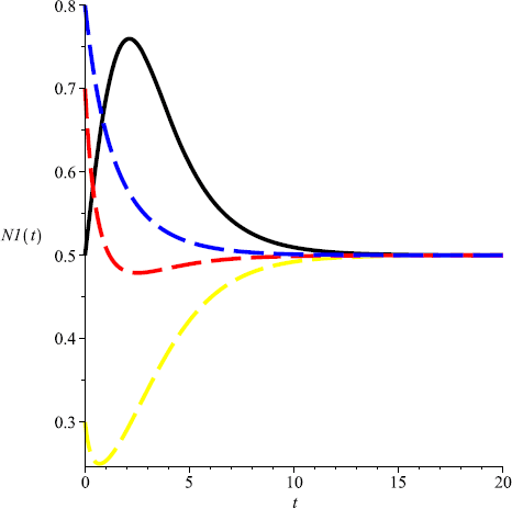
Numeric simulations of the first components of system (5.1) with \(m=0\), the initial conditions \((x(0), y(0))=(0.5,0.1), (0.8,1), (0.3, 3)\), and \((0.7,2)\), respectively
Figure 2 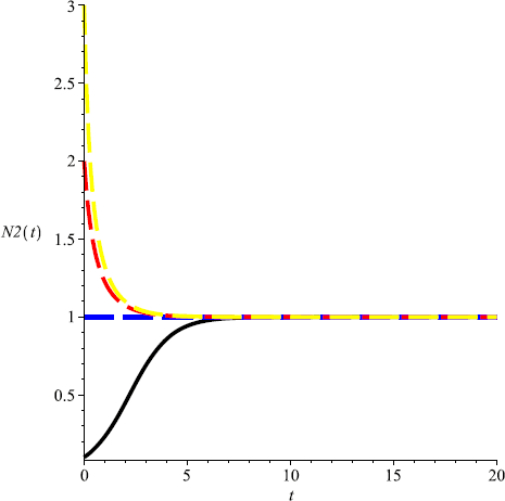
Numeric simulations of the second components of system (5.1) with \(m=0\), the initial conditions \((x(0), y(0))=(0.5,0.1), (0.8,1), (0.3, 3)\), and \((0.7,2)\), respectively
-
(2)
Take \(m=0.6\), then \(m>\max \{ \frac{r_{1}}{Eq_{1}}, \frac{r _{2}}{Eq_{2}}\}\), and both species will be driven to extinction (see Fig. 3, Fig. 4);
Figure 3 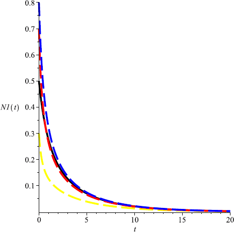
Numeric simulations of the first components of system (5.1) with \(m=0.6\), the initial conditions \((x(0), y(0))=(0.5,0.1), (0.8,1), (0.3, 3)\), and \((0.7,2)\), respectively
Figure 4 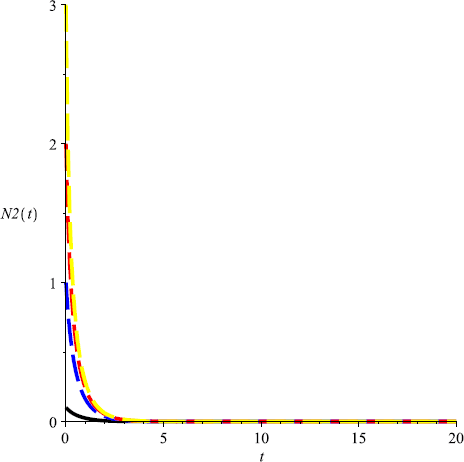
Numeric simulations of the second components of system (5.1) with \(m=0.6\), the initial conditions \((x(0), y(0))=(0.5,0.1), (0.8,1), (0.3, 3)\), and \((0.7,2)\), respectively
-
(3)
Take \(m=0.3\), then \(\frac{r_{1}}{Eq_{1}}< m< \frac{r_{2}}{Eq _{2}}\), and \(C(0, 0.4)\) is globally attractive, that is, \(N_{2}\) will be driven to extinction, and \(N_{1}\) is globally attractive (see Fig. 5, Fig. 6);
Figure 5 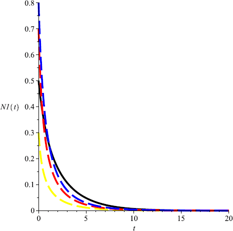
Numeric simulations of the first components of system (5.1) with \(m=0.3\), the initial conditions \((x(0), y(0))=(0.5,0.1), (0.8,1), (0.3, 3)\), and \((0.7,2)\), respectively
Figure 6 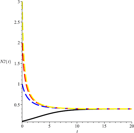
Numeric simulations of the second components of system (5.1) with \(m=0.3\), the initial conditions \((x(0), y(0))=(0.5,0.1), (0.8,1), (0.3, 3)\), and \((0.7,2)\), respectively
-
(4)
Take \(m=0.1\), then \(m<\min \{\frac{r_{2}}{Eq_{2}}, \frac{r _{1}r_{2}(P_{1}-uP_{2})}{r_{2}q_{1}EP_{1}- r_{1}uEP_{2}q_{2}} \}= \frac{1}{6}\) and \(D(0.2,0.8)\) is globally attractive, that is, both species could coexist in a stable state (see Fig. 7, Fig. 8).
Figure 7 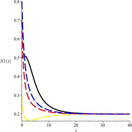
Numeric simulations of the first components of system (5.1) with \(m=0.1\), the initial conditions \((x(0), y(0))=(0.5,0.1), (0.8,1), (0.3, 3)\), and \((0.7,2)\), respectively
Figure 8 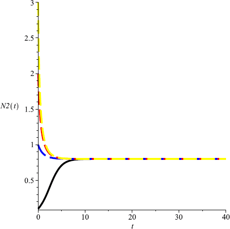
Numeric simulations of the second components of system (5.1) with \(m=0.1\), the initial conditions \((x(0), y(0))=(0.5,0.1), (0.8,1), (0.3, 3)\), and \((0.7,2)\), respectively


6 Discussion
With the aim of the ecological sustainability and conservation of the species to be implemented in a long run, in this paper, we propose a non-selective harvesting Lotka–Volterra amensalism model incorporating partial closure for the populations, i.e., system (1.2), which can be seen as the generalization of system (1.1), and the model is more suitable for the real situation.
With the introducing of harvesting, the dynamic behaviors of the system become very complicated. Depending on the fraction of the stock that could be harvested, the system may have positive equilibrium, which is globally asymptotically stable, which means that two species could coexist in a stable state; or one of the species will be driven to extinction, or both of the species could be driven to extinction.
To sum up, to ensure the conservation of the species, we need to restrict the harvesting to a limited area. Otherwise, although we can afford the area which could not be harvested, the species may still be driven to extinction. Theorem 2.1 and 3.1 give some threshold on m, which ensures the coexistence of the two species. The results obtained in this paper maybe useful in designing the natural protection area.
References
Xiong, H.H., Wang, B.B., Zhang, H.L.: Stability analysis on the dynamic model of fish swarm amensalism. Adv. Appl. Math. 5(2), 255–261 (2016)
Han, R.Y., Xue, Y.L., Yang, L.Y., et al.: On the existence of positive periodic solution of a Lotka–Volterra amensalism model. J. Rongyang Univ. 33(2), 22–26 (2015)
Chen, F.D., He, W.X., Han, R.Y.: On discrete amensalism model of Lotka–Volterra. J. Beihua Univ. (Nat. Sci.) 16(2), 141–144 (2015)
Chen, F.D., Zhang, M.S., Han, R.Y.: Existence of positive periodic solution of a discrete Lotka–Volterra amensalism model. J. Shengyang Univ. (Nat. Sci.) 27(3), 251–254 (2015)
Sun, G.C.: Qualitative analysis on two populations amensalism model. J. Jiamusi Univ. (Nat. Sci. Ed.) 21(3), 283–286 (2003)
Zhu, Z.F., Chen, Q.L.: Mathematic analysis on commensalism Lotka–Volterra model of populations. J. Jixi Univ. 8(5), 100–101 (2008)
Zhang, Z.: Stability and bifurcation analysis for a amensalism system with delays. Math. Numer. Sin. 30, 213–224 (2008)
Sita Rambabu, B., Narayan, K.L., Bathul, S.: A mathematical study of two species amensalism model with a cover for the first species by homotopy analysis method. Adv. Appl. Sci. Res. 3(3), 1821–1826 (2012)
Acharyulu, K.V.L.N., Pattabhi Ramacharyulu, N.Ch.: On the carrying capacity of enemy species, inhibition coefficient of ammensal species and dominance reversal time in an ecological ammensalism—a special case study with numerical approach. Int. J. Adv. Sci. Technol. 43, 49–57 (2012)
Xie, X.D., Chen, F.D., He, M.X.: Dynamic behaviors of two species amensalism model with a cover for the first species. J. Math. Comput. Sci. 16, 395–401 (2016)
Lin, Q.X., Zhou, X.Y.: On the existence of positive periodic solution of a amensalism model with Holling II functional response. Commun. Math. Biol. Neurosci. 2017, Article ID 3 (2017)
Wu, R.X.: A two species amensalism model with non-monotonic functional response. Commun. Math. Biol. Neurosci. 2016, Article ID 19 (2016)
Chen, F.D., Pu, L.Q., Yang, L.Y.: Positive periodic solution of a discrete obligate Lotka–Volterra model. Commun. Math. Biol. Neurosci. 2015, Article ID 14 (2015)
Wu, R.X., Zhao, L., Lin, Q.X.: Stability analysis of a two species amensalism model with Holling II functional response and a cover for the first species. J. Nonlinear Funct. Anal. 2016, Article ID 46 (2016)
Chen, L., Chen, F.: A stage-structured and harvesting predator–prey system. Ann. Appl. Math. 26(3), 293–301 (2011)
Chakraborty, K., Das, S., Kar, T.K.: On non-selective harvesting of a multispecies fishery incorporating partial closure for the populations. Appl. Comput. Math. 221, 581–597 (2013)
Chen, L., Chen, F.: Global analysis of a harvested predator–prey model incorporating a constant prey refuge. Int. J. Biomath. 3(02), 177–189 (2010)
Xie, X., Chen, F., Xue, Y.: Note on the stability property of a cooperative system incorporating harvesting. Discrete Dyn. Nat. Soc. 2014, Article ID 327823 (2014)
Chen, F.D., Wu, H.L., Xie, X.D.: Global attractivity of a discrete cooperative system incorporating harvesting. Adv. Differ. Equ. 2016, 268 (2016)
Kar, T.K., Chaudhuri, K.S.: On non-selective harvesting of a multispecies fishery. Int. J. Math. Educ. Sci. Technol. 33(4), 543–556 (2002)
Kar, T.K., Chaudhuri, K.S.: On non-selective harvesting of two competing fish species in the presence of toxicity. Ecol. Model. 161, 125–137 (2003)
Leard, B., Rebaza, J.: Analysis of predator–prey models with continuous threshold harvesting. Appl. Math. Comput. 217(12), 5265–5278 (2011)
Chakraborty, K., Das, K., Kar, T.K.: Combined harvesting of a stage structured prey-predator model incorporating cannibalism in competitive environment. C. R. Biol. 336, 34–45 (2013)
Chakraborty, K., Jana, S., Kar, T.K.: Global dynamics and bifurcation in a stage structured prey-predator fishery model with harvesting. Appl. Math. Comput. 218(18), 9271–9290 (2012)
Chen, L.S.: Mathematical Models and Methods in Ecology. Science Press, Beijing (1988) (in Chinese)
Chen, F.D.: On a nonlinear nonautonomous predator–prey model with diffusion and distributed delay. J. Comput. Appl. Math. 180(1), 33–49 (2005)
Acknowledgements
The author is grateful to anonymous referees for their excellent suggestions, which greatly improved the presentation of the paper. This work is supported by the National Social Science Foundation of China (16BKS132), Humanities and Social Science Research Project of Ministry of Education Fund (15YJA710002) and the Natural Science Foundation of Fujian Province (2015J01283).
Author information
Authors and Affiliations
Contributions
All authors contributed equally to the writing of this paper. All authors read and approved the final manuscript.
Corresponding author
Ethics declarations
Competing interests
The authors declare that there is no conflict of interests.
Additional information
Publisher’s Note
Springer Nature remains neutral with regard to jurisdictional claims in published maps and institutional affiliations.
Rights and permissions
Open Access This article is distributed under the terms of the Creative Commons Attribution 4.0 International License (http://creativecommons.org/licenses/by/4.0/), which permits unrestricted use, distribution, and reproduction in any medium, provided you give appropriate credit to the original author(s) and the source, provide a link to the Creative Commons license, and indicate if changes were made.
About this article

Cite this article
Chen, B. Dynamic behaviors of a non-selective harvesting Lotka–Volterra amensalism model incorporating partial closure for the populations. Adv Differ Equ 2018, 111 (2018). https://doi.org/10.1186/s13662-018-1555-5
Received:
Accepted:
Published:
DOI: https://doi.org/10.1186/s13662-018-1555-5