
Abstract
In this paper, we compute a common solution of the fixed point problem (FPP) and the generalized split common null point problem (GSCNPP) via the inertial hybrid shrinking approximants in Hilbert spaces. We show that the approximants can be easily adapted to various extensively analyzed theoretical problems in this framework. Finally, we furnish a numerical experiment to analyze the viability of the approximants in comparison with the results presented in (Reich and Tuyen in Rev. R. Acad. Cienc. Exactas Fís. Nat., Ser. A Mat. 114:180, 2020).
1 Introduction
The triplet \((\Xi ,\langle \cdot ,\cdot \rangle ,\|\cdot \|)\) represents a real Hilbert space, the inner product, and the induced norm, respectively. For an operator \(U:K\rightarrow K\), \(\operatorname{Fix}(U)\) denotes the set of all fixed points of the operator U, where K is a nonempty closed convex subset of Ξ. Recall that the operator U is called η-demimetric [46], where \(\eta \in (-\infty ,1)\), if \(\operatorname{Fix}(U) \neq \emptyset \) and
where Id denotes the identity operator.
The η-demimetric operator is equivalently defined by
The class of η-demimetric operators plays a prominent role in metric fixed point theory and has been analyzed in various instances of fixed point problems [47, 48, 50]. We remark that various nonlinear operators have been analyzed in connections with variational inequality problems, fixed point problems, equilibrium problems, convex feasibility problems, signal processing, and image reconstruction [3–6, 11, 12, 14–19, 23, 24, 26, 28–30, 32, 34, 35, 37, 42, 43, 53–57]. In 2007, Aoyama et al. [2] suggested a Halpern [33] type approximants for an infinite family of nonexpansive operators satisfying the AKTT-Condition \(\sum^{\infty}_{k=1}\sup_{p\in X}\Vert U_{k+1}p-U_{k}p\Vert < \infty \) for any bounded subset X of Ξ. The following construction of operator \(S_{k}\) for a countably infinite family of η-demimetric operators does not require the AKTT-Condition and hence improves the performance of the approximants:
where \(0\leq \lambda _{m}\leq 1\) and \(U^{\prime }_{m}=\rho p+(1-\rho )((1-\gamma )Id+\gamma U_{m})p\) for all \(p \in K\) with \(U_{m}\) being η-demimetric operator, \(\rho \in (0 , 1) \), and \(0<\gamma < 1-\eta \). It is well known in the context of operator \(S_{k}\) that each \(U^{\prime }_{m}\) is nonexpansive and the limit \(\lim_{k\rightarrow \infty}Q_{k,m}\) exists. Moreover,
This implies that \(\operatorname{Fix}(S)=\bigcap^{\infty}_{k=1}\operatorname{Fix}(S_{k})\) [36, 49].
The following concept of a split convex feasibility problem (SCFP) is presented in [20]:
Let H and W be nonempty closed convex subsets of real Hilbert spaces \(\Xi _{1}\) and \(\Xi _{2}\), respectively. In SCFP, we compute
where \(V: \Xi _{1} \rightarrow \Xi _{2}\) is a bounded linear operator. The SCFP is a particular case of the following split common null point problem (SCNPP) of maximal monotone operators:
Let \(A_{1}\subseteq \Xi _{1} \times \Xi _{1}\) and \(A_{2}\subseteq \Xi _{2} \times \Xi _{2}\) be two monotone operators such that \(\Gamma =A_{1}^{-1}(0)\cap V^{-1}(A_{2}^{-1}(0))\neq \emptyset \). In SCNPP, we compute \(p \in \Gamma \). Some interesting results on the SCNPP via iterative approximants can be found in [13, 21, 22, 44]. It is worth mentioning that the concept of SCNPP has been extended to the concept of a generalized split common null point problem (GSCNPP) in Hilbert spaces [39, 40]. In GSCNPP, we compute
where \(A_{j}:\Xi _{j} \rightarrow 2^{\Xi _{j}}\), \(j \in \{1,2,\ldots ,N\}\), is a finite family of maximal monotone operators, and \(V_{j}: \Xi _{j} \rightarrow \Xi _{j+1}\), \(j \in \{1,2,\ldots ,N-1\}\), is a finite family of bounded linear operators such that \(V_{j} \neq 0\).
From the perspective of optimization, problem (1.2) has been analyzed via different iterative approximants. A variant of the classical CQ-algorithm, essentially due to Byrne [13], is employed in [39], whereas shrinking projection approximants are analyzed in [40] to obtain the strong convergence results in Hilbert spaces. It is therefore natural to ask whether we can device strongly convergent approximants to compute a solution of GSCNPP and fixed point point problem of an infinite family of operators without employing the AKTT-Condition.
To answer the above question, we consider the following GSCNPP and FPP:
For the computation of a solution of problem (1.3), we employ hybrid shrinking approximants embedded with the inertial extrapolation technique, essentially due to Polyak [38] (see also [1, 7–10]), in Hilbert spaces.
The rest of the paper is organized as follows: In Sect. 2, we present mathematical preliminaries. We establish strong convergence results of the approximants and their variant, namely the Halpern-type approximants in Sect. 3. In Sect. 4, we elaborate the adaptability of the approximants for various extensively analyzed theoretical problems in this framework. Section 6 provides a numerical experiment to analyze the viability of the approximants in comparison with the existing results.
2 Preliminaries
We start this section with mathematical preliminary notions. We always assume that K is a nonempty closed convex subset of a real Hilbert space \(\Xi _{1}\).
Recall the nearest point projector \(\Pi ^{\Xi _{1}}_{K}\) of \(\Xi _{1}\) onto \(K\subset \Xi _{1}\) is defined so that for every \(p \in \Xi _{1}\), we have a unique \(\Pi ^{\Xi _{1}}_{K}p\) in K such that
Note here that the nearest point projector has the following properties:
-
(i)
\(\|\Pi ^{\Xi _{1}}_{K}p-\Pi ^{\Xi _{1}}_{K}q\|^{2}\leq \langle p-q, \Pi ^{\Xi _{1}}_{K}p-\Pi ^{\Xi _{1}}_{K}q\rangle\) for all p, \(q \in K\) (firmly nonexpansive);
-
(ii)
\(\langle p-\Pi ^{\Xi _{1}}_{K}p,\Pi ^{\Xi _{1}}_{K}p-q\rangle \geq 0\) for all \(p \in \Xi _{1}\) and \(q \in K\) (characterization property).
Let the sets \(\mathcal{D}(A_{1})=\{p \in \Xi _{1}\mid A_{1}p \neq \emptyset \}\), \(\mathcal{R}(A_{1})=\{ u \in \Xi _{1}\mid (\exists p \in \Xi _{1}) u \in A_{1}p\}\), \(\mathcal{G}(A_{1})=\{(p,u) \in \Xi _{1}\times \Xi _{1}\mid u \in A_{1}p \}\), and \(\mathcal{Z}(A_{1})=\{p \in \Xi _{1}\mid 0 \in A_{1}p\}\) denote the domain, range, graph, and zeros of a set-valued operator \(A_{1}\subseteq \Xi _{1} \times \Xi _{1}\), respectively. If a set-valued operator \(A_{1}\) satisfies \(\langle p-q,t-w\rangle \geq 0\) for all \((p,t), (q,w) \in \operatorname{gra}(A_{1})\), then \(A_{1}\) is called monotone. Recall also that a monotone operator \(A_{1}\) is called maximal monotone if its graph is not strictly contained in the graph of any other monotone operator on \(\Xi _{1}\). The well-defined single-valued operator \(\mathcal{J}^{A_{1}}_{\theta}:=(Id+\theta A_{1})^{-1}:\mathcal{R}(Id+ \theta A_{1})\rightarrow \mathcal{D}(A_{1})\) is known as the resolvent of \(A_{1}\), where \(\theta >0\). The resolvent operator \(\mathcal{J}^{A_{1}}_{\theta}\) is closely related to \(A_{1}\) as \(q \in A_{1}^{-1}(0)\) if and only if \(q=\mathcal{J}^{A_{1}}_{\theta}(q)\).
Lemma 2.1
([46])
Let \(K\subset \Xi _{1}\), and let \(U: K \rightarrow \Xi _{1}\) be an η-demimetric operator with \(\eta \in (-\infty ,1)\). Then \(\operatorname{Fix}(U)\) is closed and convex.
Lemma 2.2
([50])
Let \(K\subset \Xi _{1}\), and let \(U: K \rightarrow \Xi _{1}\) be an η-demimetric operator with \(\eta \in (-\infty ,1)\) and \(\operatorname{Fix}(U)\neq \emptyset \). Let γ be a real number such that \(0<\gamma < 1-\eta \) and set \(M=(1-\gamma )Id+\gamma U\). Then M is a quasinonexpansive operator of K into \(\Xi _{1}\).
Lemma 2.3
([45])
Let \(\Xi _{1}\) be a real Hilbert space, and let \((d_{k})\) be a sequence in \(\Xi _{1}\). Then:
-
(i)
If \(d_{k}\rightharpoonup d\) and \(\Vert d_{k}\Vert \rightarrow \Vert d \Vert \) as \(k \rightarrow \infty \), then \(d_{k} \rightarrow d\) as \(k \rightarrow \infty \) (the Kadec–Klee property);
-
(ii)
If \(d_{k} \rightharpoonup d\) as \(k \rightarrow \infty \), then \(\Vert d\Vert \leq \lim \inf_{k \rightarrow \infty}\Vert d_{k}\Vert \).
Lemma 2.4
([27])
Let \(A_{1}\subseteq \Xi _{1} \times \Xi _{1}\) be a maximal monotone operator. Then for \(\theta \geq \tilde{\theta}>0\), we have
Lemma 2.5
([31])
Let \(K\subset \Xi _{1}\). Then the operator \(Id-U\) satisfies the demiclosedness principle with respect to the origin, that is, \((Id-U)(d)=0\), provided that there exists a sequence \((d_{k})\) in K that converges weakly to some d and \(((Id-U)d_{k})\) converges strongly to 0.
Lemma 2.6
([52])
Let \(K\subset \Xi _{1}\), and let \((U^{\prime }_{m})\) be a sequence of nonexpansive operators such that \(\bigcap^{\infty}_{k=1}\operatorname{Fix}(U^{\prime }_{k}) \neq \emptyset \) and \(0\leq \beta _{m}\leq b<1\). Then for a bounded subset D of K, we have
3 Convergence analysis of the approximants
For the computation of a solution of (1.3), we propose the following approximants:
We assume the following control conditions on the approximants:
-
(C1)
\(\sum^{\infty}_{k=1}\mu _{k}\|d_{k-1}-d_{k}\|<\infty \);
-
(C2)
\(0 < a \leq \rho _{k} \leq b <1\);
-
(C3)
\(\liminf_{k \rightarrow \infty} \tau _{k} > 0\);
-
(C4)
\(\min_{j}\{\inf_{k}\{\theta _{j,k}\}\} \geq m > 0\).
Theorem 3.1
Any approximants defined via Algorithm 1, under control conditions (C1)–(C4), converge strongly to an element in Ω.

Hybrid Shrinking Approximants (Algo.1)
Proof
We divide the proof into different steps for understanding.
Step 1. We show that the approximants \((d_{k})\) defined in Algorithm 1 are stable.
Claim: \(H_{k}\) and \(W_{k}\) are closed and convex subsets of \(\Xi _{1}\) for all \(k \geq 0\).
Consider, for each \(k \geq 0\), the following representation of the subsets \(H_{k}\) and \(W_{k}\):
The claim follows from the above representations of closed and convex subsets \(H_{k}\) and \(W_{k}\) of \(\Xi _{1}\) for all \(k \geq 1\). Further, the sets Γ and \(\operatorname{Fix}(S)\) (from Lemma 2.1) are closed and convex. Hence we have that Ω is nonempty, closed, and convex. Let \(q \in \Omega \), \(\Omega \subset H_{0} = \Xi _{1}\). Now it follows from Algorithm 1 that
From (3.1) and Lemma 2.2 we obtain
This shows that Ω is contained in \(H_{k}\) for all \(k \geq 1\). Now assume that \(\Omega \subset W_{k}\) for some \(k \geq 1\). Using the nonexpansiveness of \(\mathcal{J}^{A_{j}}_{\theta _{j,k}}\), (3.1), and (3.2), we get
It follows from estimate (3.3) that \(\Omega \subset W_{k+1}\), and hence \(\Omega \subset H_{k+1}\cap W_{k+1}\). Consequently, by Step 1 the approximants \((d_{k})\) defined in Algorithm 1 are stable.
Step 2. We next show that \(\lim_{k\rightarrow \infty }\Vert d_{k}-d_{1}\Vert \) exists.
Observe that
since \(d_{k+1}=\Pi ^{\Xi _{1}}_{H_{k+1}\cap W_{k+1}}d_{1}\). In particular,
These estimates establish the boundedness of the approximants \((\Vert d_{k}-d_{1}\Vert )\). Since \(d_{k}=\Pi ^{\Xi _{1}}_{H_{k}\cap W_{k}}d_{1}\) and \(d_{k+1}=\Pi ^{\Xi _{1}}_{H_{k+1}\cap W_{k+1}}d_{1} \in H_{k+1}\), we have
This yields that the approximants \((\Vert d_{k}-d_{1}\Vert )\) are nondecreasing, and hence
Step 3. We now show that \(\tilde{q}\in \Omega \).
We first compute
By (3.3) the above computation yields
In view of the control condition (C1), we get
As a consequence of estimates (3.5) and (3.6), we also obtain that
Since \(d_{k+1} \in H_{k+1}\), we have
This estimate, in the light of estimate (3.5) and the control condition (C1), yields that
Similarly, we infer from estimates (3.5) and (3.8) that
and from the estimates (3.6) and (3.9) that
In view of the control condition (C2), consider the variant of estimate (3.2)
Letting \(k \rightarrow \infty \) and using (3.9) and (C2), we have
Observe that
The above computation, in view of estimates (3.10) and (3.11), yields
Note that \(d_{k+1}=\Pi ^{\Xi _{1}}_{H_{k}\cap W_{k}}(d_{1}) \in W_{k}\). Therefore we have
Employing estimate (3.8), the above computation yields
Reasoning as above, we infer from estimates (3.8) and (3.13) that
and from estimates (3.9) and (3.14) that
Since \((d_{k})\) is bounded, there exists a subsequence \((d_{k_{t}})\) of \((d_{k})\) such that \(d_{k_{t}} \rightharpoonup \tilde{q} \in \Xi _{1}\) as \(t \rightarrow \infty \). Therefore \(b_{k_{t}} \rightharpoonup \tilde{q}\) and \(c_{k_{t}}\rightharpoonup \bar{V}_{j-1}\tilde{q}\) as \(t \rightarrow \infty \). From the definition of \(\bar{V}_{j-1}\) we have \(\bar{V}_{j-1}d_{k_{t}}\rightharpoonup \bar{V}_{j-1}\tilde{q}\) as \(t \rightarrow \infty \) for all \(j \in \{1,2,\ldots ,N\}\).
Using (3.14), we estimate that
for all \(j \in \{1,2,\ldots ,N\}\). Then from Lemma 2.4 and (C4) we obtain the inequality
This estimate implies that
for all \(j \in \{1,2,\ldots ,N\}\). By Lemma 2.5 we have \(\bar{V}_{j-1}\tilde{q} \in \operatorname{Fix}(\mathcal{J}^{A_{j}}_{\theta})\) for all \(j \in \{1,2,\ldots ,N\}\), that is, \(\tilde{q} \in \Gamma \). It remains to show that \(\tilde{q} \in \operatorname{Fix}(S)\). Observe that
Using (3.12) and Lemma 2.6, this estimate implies that \(\lim_{k\rightarrow \infty}\Vert b_{k}-Sb_{k}\Vert =0\). This, together with the fact that \(b_{k_{t}} \rightharpoonup \tilde{q}\), implies by Lemma 2.5 that \(\tilde{q} \in \operatorname{Fix}(S)= \bigcap^{\infty}_{k=1}\operatorname{Fix}(S_{k})\). Hence \(\tilde{q} \in \Omega \).
Step 4. The final part is showing that \(d_{k}\rightarrow q=\Pi ^{\Xi _{1}}_{\Omega }d_{1}\).
Since \(q=\Pi ^{\Xi _{1}}_{\Omega}d_{1}\) and \(\tilde{q} \in \Omega \), Lemma 2.3 implies that
Using the uniqueness of q yields the equality \(\tilde{q}=q\). From Step 2 it follows that \(\Vert d_{k_{t}}-d_{1}\Vert \leq \Vert q-d_{1}\Vert \), and from Lemma 2.3 we obtain \(\lim_{k\rightarrow \infty }d_{k}=\tilde{q}=q=\Pi ^{\Xi _{1}}_{ \Omega }d_{1}\). □
We first apply Theorem 3.1 to the following problem:
where \(A_{j}\subseteq \Xi _{1} \times \Xi _{1}\), \(j\in \{1,2,\ldots ,s\}\), and \(A_{\ell}\subseteq \Xi _{1} \times \Xi _{1}\), \(\ell =\{s+1,s+2,\ldots ,N\}\), are finite families of maximal monotone operators, and \(S_{k}:\Xi _{1} \rightarrow \Xi _{1}\) is an infinite family of η-demimetric operators.
Corollary 3.2
Assume that \(\Omega \neq \emptyset \). Then the approximants initialized by arbitrary \(d_{0}, d_{1} \in \Xi _{1}\) and \(H_{0}= W_{0} = \Xi _{1}\) with the nonincreasing sequences \(\rho _{k},\tau _{k} \subset (0,1)\), \(\mu _{k} \in [0,1)\), and \(\gamma _{k} \in (0, \infty )\) for \(k\geq 1\) defined as
under the control conditions (C1)–(C4), converge strongly to an element in Ω.
We now consider the following Halpern-type variant of Algorithm 1:
Theorem 3.3
Any approximants defined via Algorithm 2, under the control conditions (C1)–(C4), converge strongly to an element in Ω.

Hybrid Shrinking Halpern Approximants (Algo.2)
Proof
Observe that for each \(k \geq 1\), the subsets \(H_{k}\) have the following form:
Arguing similarly as in the proof of Theorem 3.1 (Steps 1–2), we deduce that Ω, \(H_{k}\), and \(W_{k}\) are closed and convex. Moreover, \(\Omega \subset H_{k+1}\cap W_{k+1}\) for all \(k \geq 1\). Furthermore, the sequence \((d_{k})\) is bounded, and
Since \(d_{k+1}=\Pi ^{\Xi _{1}}_{H_{k}\cap W_{k}}(t) \in H_{k}\), we have
Letting \(k \rightarrow \infty \), using (3.18) along (C1)–(C2), and the boundedness of \((d_{k})\), we obtain
Similarly, we get
Let \(b_{k}=\rho _{k}t+(1-\rho _{k})S_{k}a_{k}\). An easy calculation along (C1)–C2) implies that
This estimate implies that
The rest of the proof of Theorem 3.3 follows immediately from the proof of Theorem 3.1 and is therefore omitted. □
4 Applications
Our main result in the previous section has various interesting applications of great importance in the field. We present some of these applications.
4.1 Generalized split feasibility problems
In the context of generalized split feasibility problems [20], we recall that the indicator function \(j_{K}\) is a proper lower semicontinuous convex function (PCLS), where \(K\subset \Xi _{1}\). Therefore \(\partial j_{K}\), the subdifferential of \(j_{K}\), satisfies the maximal monotonicity such that \(\partial j_{K}(p)=N_{p}^{K}\), where \(N_{p}^{K}\) denotes the normal cone of K at u. From this we can deduce that \(\partial j_{K}\) coincides with \(\Pi _{K}^{\Xi _{1}}\). Assume that
where \(K_{j}\subset \Xi _{j}\), \(j \in \{1,2,\ldots ,N\}\).
Theorem 4.1
Assume that \(\Omega = \Theta \cap \operatorname{Fix}(S)\neq \emptyset \). Then the approximants initialized by arbitrary \(d_{0}, d_{1} \in \Xi _{1}\) and \(H_{0}= W_{0}=\Xi _{1}\) with the nonincreasing sequences \(\rho _{k},\tau _{k} \subset (0,1)\), \(\mu _{k} \in [0,1)\), and \(\gamma _{k} \in (0, \infty )\) for \(k\geq 1\) defined as
under the control conditions (C1)–(C4), converge strongly to an element in Ω.
4.2 Generalized split variational inequality problems
The well-known variational inequality problem deals with computation of a point \(p \in K\) such that
where \(\mathcal{A}:K \rightarrow \Xi _{1}\) is a nonlinear monotone operator defined with respect to \(K\subset \Xi _{1}\). By \(\operatorname{Sol}(K,\mathcal{A})\) we denote the set of all solutions associated with the variational inequality problem. We consider the following problem:
Theorem 4.2
Assume that \(\Omega = \Theta \cap \operatorname{Fix}(S)\neq \emptyset \). Then the approximants initialized by arbitrary \(d_{0}, d_{1} \in \Xi _{1}\) and \(H_{0}= W_{0}=\Xi _{1}\) with the nonincreasing sequences \(\rho _{k},\tau _{k} \subset (0,1)\), \(\mu _{k} \in [0,1)\), and \(\gamma _{k} \in (0, \infty )\) for \(k\geq 1\) defined as
under the control conditions (C1)–(C4), converge strongly to an element in Ω.
Proof
Let \(h_{\mathcal{A}_{j}}\subset \Xi _{j} \times \Xi _{j}\) be defined by
where \(N_{K_{j}}(p):=\{q \in \Xi _{j}:\langle t-p, q\rangle \leq 0 \text{ for all } t \in K_{j}\}\), \(j=\{1,2,\ldots ,N\}\).
Note that \(h_{\mathcal{A}_{j}}\) is maximal monotone [41] such that
The rest of the proof now follows from Theorem 3.1. □
4.3 Generalized split minimization problems
Let the set of minimizers associated with the function \(\phi : \Xi _{1} \rightarrow (-\infty ,\infty ]\) be denoted as
If ϕ is a proper convex lower semicontinuous (PCLS) function, then ∂ϕ is a maximal monotone operator. Moreover, \(q \in (\partial \phi )^{-1}0 \Leftrightarrow 0 \in \partial \phi (q)\) (see [25]). Now observe that
where \(\phi _{j}: \Xi _{j} \rightarrow (-\infty ,\infty ]\) is as defined above.
Theorem 4.3
Assume that \(\Omega = \Theta \cap \operatorname{Fix}(S) \neq \emptyset\). Then the approximants initialized by arbitrary \(d_{0}, d_{1} \in \Xi _{1}\) and \(H_{0}= W_{0}=\Xi _{1}\) with the nonincreasing sequences \(\rho _{k},\tau _{k} \subset (0,1)\), \(\mu _{k} \in [0,1)\), and \(\gamma _{k} \in (0, \infty )\) for \(k\geq 1\) defined as
under the control conditions (C1)–(C4), converge strongly to an element in Ω.
4.4 Signal processing
This subsection deals with the case of signal recovery problem, which we aim to solve by applying Theorem 4.1. The following underdetermined formalism denotes the signal recovery problem:
where \(\kappa \in \mathbb{R}^{M}\) is the measured noise data with noise ϑ, \(d \in \mathbb{R}^{N}\) is the sparse original data for recovery, and \(V:\mathbb{R}^{N} \rightarrow \mathbb{R}^{M}\) (\(M < N\)) is the bounded linear observation matrix. Formalism (4.4) is equivalent to the well-known least absolute shrinkage and selection operator (LASSO) problem [51] in the following convex constrained optimization formalism:
If we set \(\Theta = K_{1}\cap V^{-1}(K_{2}) \neq \emptyset \) with \(K_{1}=\{d \mid t\geq \Vert d\Vert _{1} \}\) and \(K_{2}=\{\kappa \}\), then the LASSO problem can be easily solved via Theorem 4.1. To conduct the numerical experiment, we generate (i) the matrix \(V^{N \times M}\) from the standard normal distributions with zero mean and unit variance, (ii) d having \(m\ll N\) nonzero elements via a uniform distribution in \([-2,2]\), and (iii) κ from a Gaussian noise with signal-to-noise ratio \(\mathrm{SNR} =40\). The approximants are initiated with randomly chosen \(d_{0}\), \(d_{1}\) and abort when the following mean square error is satisfied:
Here \(d^{\ast}\) is called the estimated signal of d.
For Theorem 4.1, we choose \(\mu _{k} =\frac{1}{(100 \times k+1)^{1.04}}\), \(\rho _{k} =\frac{1}{k^{1.02}}\), \(t=m-0.001\), and \(\vartheta =0\).
We recover the signals for the following two tests:
Numerical Test 1
Choose \(N=512\), \(M=256\), and \(m=15\).
Numerical Test 2
Choose \(N=1024\), \(M=512\), and \(m=30\).
From Table 1 and Figs. 1 and 2 we conclude that IGSNPP as in Theorem 4.1 reconstruct the original signal (A) faster than the algorithm for GSNPP as in Theorem 4.4 [40] in the compressed sensing. Moreover, the graph of error function values (B) and objective function values (C) generated by IGSNPP as in Theorem 4.1 converge faster as compared to the algorithm for GSNPP as in Theorem 4.4 [40].

Comparison of two algorithms for Numerical Test 1

Comparison of two algorithms for Numerical Test 2
5 Numerical experiment and results
In this section, we focus on numerical implementation of our proposed algorithm. Comparison with Reich et al. [40]) shows the effectiveness and efficiency of our proposed algorithm. All codes were written in MATLAB R2020a and performed on a laptop Intel(R) Core(TM) i3-3217U @ 1.80 GHz, RAM 4.00 GB.
Example 5.1
Let \(\Xi _{1} = \mathbb{R}^{2}\) and \(\Xi _{2} = \mathbb{R}^{4}\) with the inner product defined by \(\langle x, y\rangle = xy\), for all \(x , y \in \mathbb{R}^{2},\mathbb{R}^{4}\) and the induced usual norm \(|\cdot |\).
Consider the following problem: find an element \(q \in \mathbb{R}^{2}\) such that
where
and \(V:\mathbb{R}^{2}\rightarrow \mathbb{R}^{4}\) is a bounded linear matrix randomly generated in the closed interval \([-5,5]\). Let the operators \(S_{k}: \mathbb{R}^{2} \rightarrow \mathbb{R}^{2}\) be defined by \(S_{k}(x)= (-(k+1)x_{1},-(k+1)x_{2})\) for \(k=1,2\). Then \(S_{k}\) is a η-demimetric operator with \(\eta _{1}=\frac{1}{3}\) and \(\eta _{2}=\frac{1}{2}\), respectively. It is easy to observe that \(\bigcap_{k=1}^{2} \operatorname{Fix}(S_{k})=\{0\}\) and \(\Theta := \{\Theta _{1}\cap V^{-1}(\Theta _{2})\}=0\). Hence \(\Omega = \Theta \cap \operatorname{Fix}(S) = 0\). Furthermore, the coordinate of the center a is randomly generated in the closed interval \([-1,1]\), and the radii \(R_{1}\) and \(R_{2}\) are randomly generated in the closed intervals \([5,9]\) and \([9,17]\), respectively. The coordinates of the initial point \(d_{0}\), \(d_{1}\) are randomly generated in the closed interval \([-5,5]\). Choose \(\mu =0.9\), \(m=0.01\), \(\rho _{k} =\frac{1}{100k+1}\), and \(\beta _{1} =\frac{1}{100k+1}\). We provide a numerical test of the hybrid shrinking approximants defined in Theorem 4.1 (i.e., Theorem 4.1 with \(\mu _{k}\neq 0\)) with the noninertial variant of Theorem 4.4 (i.e., Theorem 4.4, Reich et al. [40]). It is remarked that the function \(E_{k}\) is defined by
Note that at the kth step, \(E_{k}=0\), and then \(d_{k}\in \Theta \), which implies that \(d_{k}\) is a solution of this problem. The stopping criterion is defined as \(E_{k} < 10^{-5}\). The different choices of \(d_{0}\), \(d_{1}\) are given as follows:
-
Case I:
\(d_{0}=[6,8]^{T}\), \(d_{1}=[3,7]^{T}\).
-
Case II:
\(d_{0}=[6.5,7.2]^{T}\), \(d_{1}=[-1.4,-9.7]^{T}\).
-
Case III:
\(d_{0}=[3,-4.7]^{T}\), \(d_{1}=[1.2,4]^{T}\).
Remark 5.2
-
(i)
The example presented above serves for two purposes:
-
impact of different values of \(\mu _{k}\) on our proposed algorithm
-
comparison with the noninertial (\(\mu _{k} = 0\)) type algorithm proposed by Reich et al. [40] given in Theorem 4.4.
-
-
(ii)
The numerical results presented in Table 2 and Figs. 3–5 indicate that our proposed approximants are efficient, easy to implement, and do well for any values of \(\mu _{k}\neq 0\) in both number of iterations and CPU time required.
Figure 3 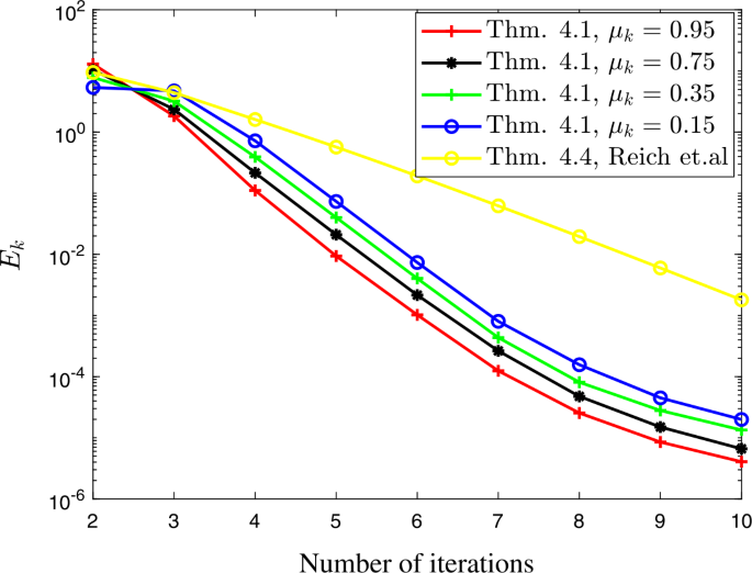
Example 5.1: Case I
Figure 4 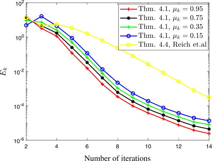
Example 5.1: Case II
Figure 5 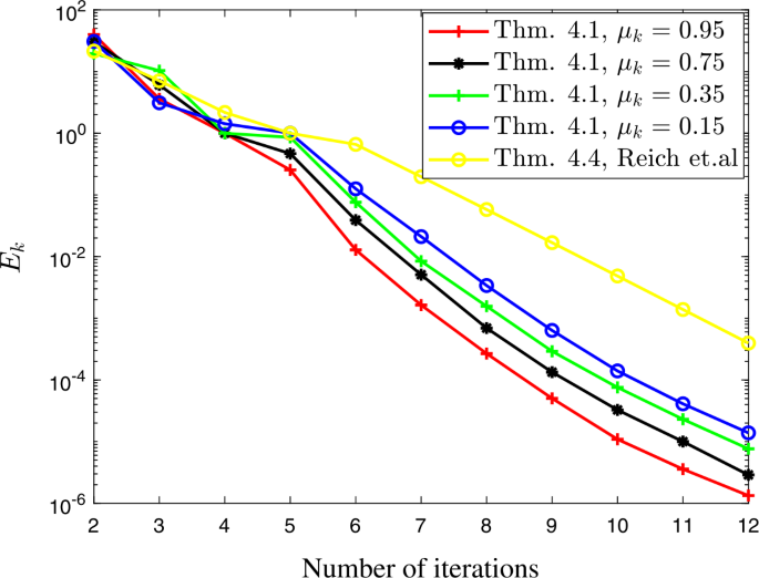
Example 5.1: Case III
-
(iii)
We observe that the CPU time of Theorem 4.1 increases, but the number of iterations decreases as the parameter μ approaches 1.
-
(iv)
We observe from the numerical implementation above and our proposed algorithm outperformed the noninertial version proposed by Reich et al. [40] given in Theorem 4.4 both in the number of iterations and CPU time required to reach the stopping criterion.


6 Conclusions
The problem for computing a common solution via unifying approximants, of a finite family of GSCNPP and the FPP for a countably infinite family of nonlinear operators has its own importance in the fields of monotone operator theory and fixed point theory. We proved that the approximants perform in an effective and efficient way when compared with the existing approximants, in particular, those studied in Hilbert spaces. The theoretical framework of the algorithm has been strengthened with an appropriate numerical example. Moreover, this framework has also been implemented to various instances of the split inverse problems. We would like to emphasize that the above mentioned problems occur naturally in many applications. Therefore iterative algorithms are inevitable in this field of investigation. As a consequence, our theoretical framework constitutes an important topic of future research.
Availability of data and materials
Data sharing not applicable to this paper as no datasets were generated or analyzed during the current study.
References
Alvarez, F., Attouch, H.: An inertial proximal method for monotone operators via discretization of a nonlinear oscillator with damping. Set-Valued Anal. 9, 3–11 (2001)
Aoyama, K., Kimura, Y., Takahashi, W., Toyoda, M.: Approximation of common fixed points of a countable family of nonexpansive mappings in a Banach space. Nonlinear Anal. 67, 2350–2360 (2007)
Arfat, Y., Kumam, P., Khan, M.A.A., Iyiola, O.S.: Multi-inertial parallel hybrid projection algorithm for generalized split null point problems. J. Appl. Math. Comput. (2021). https://doi.org/10.1007/s12190-021-01660-4
Arfat, Y., Kumam, P., Khan, M.A.A., Ngiamsunthorn, P.S.: Parallel shrinking inertial extragradient approximants for pseudomonotone equilibrium, fixed point and generalized split null point problem. Ric. Mat. (2021). https://doi.org/10.1007/s11587-021-00647-4
Arfat, Y., Kumam, P., Khan, M.A.A., Ngiamsunthorn, P.S.: Shrinking approximants for fixed point problem and generalized split null point problem in Hilbert spaces. Optim. Lett. (2021). https://doi.org/10.1007/s11590-021-01810-4
Arfat, Y., Kumam, P., Khan, M.A.A., Ngiamsunthorn, P.S.: An accelerated visco-Cesaro means Tseng type splitting method for fixed point and monotone inclusion problems. Carpath. J. Math. 38(2), 281–297 (2022)
Arfat, Y., Kumam, P., Khan, M.A.A., Ngiamsunthorn, P.S., Kaewkhao, A.: An inertially constructed forward-backward splitting algorithm in Hilbert spaces. Adv. Differ. Equ. 2021, 124 (2021)
Arfat, Y., Kumam, P., Khan, M.A.A., Ngiamsunthorn, P.S., Kaewkhao, A.: A parallel hybrid accelerated extragradient algorithm for pseudomonotone equilibrium, fixed point, and split null point problems. Adv. Differ. Equ. 2021, 364 (2021)
Arfat, Y., Kumam, P., Ngiamsunthorn, P.S., Khan, M.A.A.: An inertial based forward-backward algorithm for monotone inclusion problems and split mixed equilibrium problems in Hilbert spaces. Adv. Differ. Equ. 2020, 453 (2020)
Arfat, Y., Kumam, P., Ngiamsunthorn, P.S., Khan, M.A.A.: An accelerated projection based parallel hybrid algorithm for fixed point and split null point problems in Hilbert spaces. Math. Methods Appl. Sci., 1–19 (2021). https://doi.org/10.1002/mma.7405
Bauschke, H.H., Combettes, P.L.: Convex Analysis and Monotone Operator Theory in Hilbert Spaces. Springer, Berlin (2017)
Bauschke, H.H., Matoušková, E., Reich, S.: Projection and proximal point methods: convergence results and counterexamples. Nonlinear Anal. 56, 715–738 (2004)
Byrne, C.: A unified treatment of some iterative algorithms in signal processing and image reconstruction. Inverse Probl. 20(1), 103–120 (2004)
Cai, G., Gibali, A., Iyiola, O.S., Shehu, Y.: A new double-projection method for solving variational inequalities in Banach spaces. J. Optim. Theory Appl. 178(1), 219–239 (2018)
Ceng, L.C., Coroian, I., Qin, X., Yao, J.C.: A general viscosity implicit iterative algorithm for split variational inclusions with hierarchical variational inequality constraints. Fixed Point Theory 20, 469–482 (2019)
Ceng, L.C., Li, X., Qin, X.: Parallel proximal point methods for systems of vector optimization problems on Hadamard manifolds without convexity. Optimization 69, 357–383 (2020)
Ceng, L.C., Petrusel, A., Qin, X., Yao, J.C.: A modified inertial subgradient extragradient method for solving pseudomonotone variational inequalities and common fixed point problems. Fixed Point Theory 21, 93–108 (2020)
Ceng, L.C., Shang, M.J.: Hybrid inertial subgradient extragradient methods for variational inequalities and fixed point problems involving asymptotically nonexpansive mappings. Optimization 70, 715–740 (2021)
Ceng, L.C., Yuan, Q.: Composite inertial subgradient extragradient methods for variational inequalities and fixed point problems. J. Inequal. Appl. 2019, 274 (2019). https://doi.org/10.1186/s13660-019-2229-x
Censor, Y., Elfving, T.: A multiprojection algorithm using Bregman projections in a product space. Numer. Algorithms 8, 221–239 (1994)
Censor, Y., Elfving, T., Kopf, N., Bortfeld, T.: The multiple-sets split feasibility problem and its applications. Inverse Probl. 21, 2071–2084 (2005)
Censor, Y., Gibali, A., Reich, S.: Algorithms for the split variational inequality problem. Numer. Algorithms 59, 301–323 (2012)
Chen, J.Z., Ceng, L.C., Qiu, Y.Q., Kong, Z.R.: Extra-gradient methods for solving split feasibility and fixed point problems. Fixed Point Theory Appl. 2015, 192 (2015)
Combettes, P.L.: The convex feasibility problem in image recovery. Adv. Imaging Electron Phys. 95, 155–453 (1996)
Combettes, P.L., Pesquet, J.C.: Proximal splitting methods in signal processing. In: Fixed-Point Algorithms for Inverse Problems in Science and Engineering, pp. 185–212 (2011)
Cui, H.H., Ceng, L.C.: Iterative solutions of the split common fixed point problem for strictly pseudo-contractive mappings. J. Fixed Point Theory Appl. 20, 92 (2018)
Cui, H.H., Su, M.: On sufficient conditions ensuring the norm convergence of an iterative sequence to zeros of accretive operators. Appl. Math. Comput. 258, 67–71 (2015)
Cui, H.H., Zhang, H.X., Ceng, L.C.: An inertial Censor–Segal algorithm for split common fixed-point problems. Fixed Point Theory Appl. 22, 93–103 (2021)
Dong, Q.L., Liu, L., Yao, Y.: Self-adaptive projection and contraction methods with alternated inertial terms for solving the split feasibility problem. J. Nonlinear Convex Anal. 23(3), 591–605 (2022)
Dong, Q.L., Peng, Y., Yao, Y.: Alternated inertial projection methods for the split equality problem. J. Nonlinear Convex Anal. 22, 53–67 (2021)
Goebel, K., Kirk, W.A.: Topics in Metric Fixed Point Theory. Cambridge Studies in Advanced Mathematics. Cambridge University Press, Cambridge (1990)
Guan, J.L., Ceng, L.C., Hu, B.: Strong convergence theorem for split monotone variational inclusion with constraints of variational inequalities and fixed point problems. J. Inequal. Appl. 2018, 311 (2018)
Halpern, B.: Fixed points of nonexpansive maps. Bull. Am. Math. Soc. 73, 957–961 (1967)
Iyiola, O.S., Shehu, Y.: Alternated inertial method for nonexpansive mapping with applications. J. Nonlinear Convex Anal. 21(5), 1175–1189 (2020)
Jantakarn, K., Kaewcharoen, A.: A Bregman hybrid extragradient method for solving pseudomonotone equilibrium and fixed point problems. J. Nonlinear Funct. Anal. 2022(6) (2022)
Komiya, H., Takahashi, W.: Strong convergence theorem for an infinite family of demimetric mappings in a Hilbert space. J. Convex Anal. 24(4), 1357–1373 (2017)
Liu, L., Cho, S.Y., Yao, J.C.: Convergence analysis of an inertial Tseng’s extragradient algorithm for solving pseudomonotone variational inequalities and applications. J. Nonlinear Var. Anal. 5, 627–644 (2021)
Polyak, B.T.: Some methods of speeding up the convergence of iteration methods. USSR Comput. Math. Math. Phys. 4(5), 1–17 (1964)
Reich, S., Tuyen, T.M.: Iterative methods for solving the generalized split common null point problem in Hilbert spaces. Optimization 69, 1013–1038 (2019)
Reich, S., Tuyen, T.M.: Parallel iterative methods for solving the generalized split common null point problem in Hilbert spaces. Rev. R. Acad. Cienc. Exactas Fís. Nat., Ser. A Mat. 114, 180 (2020)
Rockafellar, R.T.: On the maximality of sums of nonlinear monotone operators. Trans. Am. Math. Soc. 149, 75–88 (1970)
Shehu, Y., Iyiola, O.S., Ogbuisi, F.U.: Iterative method with inertial terms for nonexpansive mappings: applications to compressed sensing. Numer. Algorithms 83(4), 1321–1347 (2020)
Shehu, Y., Iyiola, O.S., Reich, S.: A modified inertial subgradient extragradient method for solving variational inequalities. Optim. Eng. 23, 421–449 (2022)
Takahashi, S., Takahashi, W.: The split common null point problem and the shrinking projection method in Banach spaces. Optimization 65, 281–287 (2016)
Takahashi, W.: Nonlinear Functional Analysis: Fixed Point Theory and Its Applications. Yokohama Publishers, Yokohama (2000)
Takahashi, W.: The split common fixed point problem and the shrinking projection method in Banach spaces. J. Convex Anal. 24, 1015–1028 (2017)
Takahashi, W.: Strong convergence theorem for a finite family of demimetric mappings with variational inequality problems in a Hilbert space. Jpn. J. Ind. Appl. Math. 34, 41–57 (2017)
Takahashi, W.: Weak and strong convergence theorems for new demimetric mappings and the split common fixed point problem in Banach spaces. Numer. Funct. Anal. Optim. 39(10), 1011–1033 (2018)
Takahashi, W., Shimoji, K.: Convergence theorems for nonexpansive mappings and feasibility problems. Math. Comput. Model. 32, 1463–1471 (2000)
Takahashi, W., Wen, C.F., Yao, J.C.: The shrinking projection method for a finite family of demimetric mappings with variational inequality problems in a Hilbert space. Fixed Point Theory 19, 407–419 (2018)
Tibshirani, R.: Regression shrinkage and selection via LASSO. J. R. Stat. Soc., Ser. B 58, 267–288 (1996)
Wang, S.: A general iterative method for obtaining an infinite family of strictly pseudo-contractive mappings in Hilbert spaces. Appl. Math. Lett. 24, 901–907 (2011)
Xiao, J., Huang, L., Wang, Y.: Strong convergence of modified inertial Halpern simultaneous algorithms for a finite family of demicontractive mappings. Appl. Set-Valued Anal. Optim. 2, 317–327 (2020)
Yao, Y., Liou, Y.C., Postolache, M.: Self-adaptive algorithms for the split problem of the demicontractive operators. Optimization 67, 1309–1319 (2018)
Yao, Y., Liou, Y.C., Yao, J.C.: Split common fixed point problem for two quasi pseudo contractive operators and its algorithm construction. Fixed Point Theory Appl. 2015, 127 (2015)
Yao, Y., Liou, Y.C., Yao, J.C.: Iterative algorithms for the split variational inequality and fixed point problems under nonlinear transformations. J. Nonlinear Sci. Appl. 10, 843–854 (2017)
Yao, Y., Yao, J.C., Liou, Y.C., Postolache, M.: Iterative algorithms for split common fixed points of demicontractive operators without priori knowledge of operator norms. Carpath. J. Math. 34, 459–466 (2018)
Acknowledgements
The authors wish to thank the anonymous referees for their comments and suggestions. Yasir Arfat was supported by the Petchra Pra Jom Klao PhD Research Scholarship from King Mongkut’s University of Technology Thonburi, Thailand (Grant No. 16/2562).
Funding
The authors acknowledge the financial support provided by the Center of Excellence in Theoretical and Computational Science (TaCS-CoE), KMUTT. Moreover, this reserch was funded by King Mongkut’s University of Technology North Bangkok, Contract No. KMUTNB-65-KNOW-28.
Author information
Authors and Affiliations
Contributions
Conceptualization of the paper was carried out by YA, MA, and PK. Methodology by YA and MA. Formal analysis, investigation, and writing the original draft preparation by YA, MA and OS. Software and validation by OS, WK and KS. Writing, reviewing, and editing by YA, MA, and PK. Project administration by PK, WK, and KS. All authors read and approved the final manuscript.
Corresponding author
Ethics declarations
Competing interests
The authors declare that they have no competing interests.
Rights and permissions
Open Access This article is licensed under a Creative Commons Attribution 4.0 International License, which permits use, sharing, adaptation, distribution and reproduction in any medium or format, as long as you give appropriate credit to the original author(s) and the source, provide a link to the Creative Commons licence, and indicate if changes were made. The images or other third party material in this article are included in the article’s Creative Commons licence, unless indicated otherwise in a credit line to the material. If material is not included in the article’s Creative Commons licence and your intended use is not permitted by statutory regulation or exceeds the permitted use, you will need to obtain permission directly from the copyright holder. To view a copy of this licence, visit http://creativecommons.org/licenses/by/4.0/.
About this article

Cite this article
Arfat, Y., Iyiola, O.S., Khan, M.A.A. et al. Convergence analysis of the shrinking approximants for fixed point problem and generalized split common null point problem. J Inequal Appl 2022, 67 (2022). https://doi.org/10.1186/s13660-022-02803-2
Received:
Accepted:
Published:
DOI: https://doi.org/10.1186/s13660-022-02803-2