
Abstract
The pole-skipping phenomenon is a special property of the retarded Green’s function of black hole perturbations. We turn to its analog in acoustic black holes, which may relate to experiments. The frequencies of these special points are located at negative integer (imaginary) Matsubara frequencies \(\omega =-i2\pi Tn\), which are consistent with the imaginary frequencies of quasinormal modes (QNMs). This implies that the lower-half plane pole-skipping phenomena have the same physical meaning as the imaginary part of QNMs, which represents the dissipation of perturbation of acoustic black holes and is related to the instability time scale of perturbation.
1 Introduction
The retarded Green’s function is not unique at a special point in complex momentum space \((\omega ,k)\) and this phenomenon is known as “pole-skipping” [1,2,3]. The retarded Green’s function is given by
The location of the special points makes the coefficient \(a(\omega _\star , k_\star )=b(\omega _\star , k_\star )=0\). Then, the retarded Green’s function becomes \(G^R(\omega _\star , k_\star )=0/0\). So if we find the intersection of zeros and poles in the retarded Green’s functions, we can obtain these special points. We can use the simpler method, the AdS/CFT duality, to solve special points from the bulk field equation [4,5,6,7]. On the bulk side, the non-uniqueness of the incoming mode at the horizon corresponds to the nonuniqueness of the Green’s function on the boundary.
The upper-half \(\omega \)-plane special point contains the information of quantum chaos. We can extract the Lyapunov exponent \(\uplambda \) and the butterfly velocity \(v_B\) from it. Although the special points located at the lower-half \(\omega \)-plane are not related to the information of quantum chaos, the retarded Green’s functions are also not unique at these special points. The general pole-skipping points in the lower-half \(\omega \)-plane are located at negative integer (imaginary) Matsubara frequencies \({\mathfrak {w}}_{n}=-in\) \((n=1,2\dots )\), where \({\mathfrak {w}}=\frac{\omega }{2\pi T}\). These special points have been found in BTZ black hole [6], Schwarzschild-AdS spacetime [7], 2D CFT [8], a holographic system with the chiral anomaly [9], a holographic system at finite chemical potential [10], hyperbolic space [11, 12], the large q limit of SYK chain [13], anisotropic plasma [14], Lifshitz, and Rindler geometries [15]. However, the physical interpretation of the pole-skipping phenomenon remains elusive. Further investigations of the pole-skipping phenomenon in a different scenario and its possible connections to the experiments are of significant interest.
Analogue black holes provide new windows of looking at problems between astrophysical phenomena with tabletop experiments. Using hydrodynamical flows as analogous systems to mimic a few properties of black hole physics has been proposed in [16]. Sound waves in a moving fluid could, in principle, analogize light waves in curved spacetime. “Acoustic (sonic) black hole” (ABH) shows that sound waves cannot escape from the acoustic horizon. The horizon, ergo-sphere, and Hawking radiation of \((3+1)\)-dimensional static and rotating acoustic black holes have been studied in [17]. Some authors construct a general acoustic regular black hole that gives rise to a non-vanishing partition function that coincides with that of a conformally related black hole [18]. Acoustic black holes for relativistic fluids can also be derived from the Abelian Higgs model [19,20,21]. The acoustic black holes might be created in high-energy physical processes [22]. In Ref. [23], the authors analyze the horizon structure of the acoustic charged black hole in curved spacetime. ABH provides a concrete laboratory model for curved space quantum field theory that we can experiment. The analogue model reflects important features of general relativity and gravity.
Perturbations of classical gravitational backgrounds involving black holes naturally lead to quasinormal modes (QNMs) which are eigenmodes of dissipative systems. The eigenfrequencies \(\omega _{QNM}\) have both a real and an imaginary part, with the real part denotes the amplitude and the imaginary part denotes the mode’s damping time, which is associated with the decay timescale of the perturbation [24,25,26].
In [15], we obtain the “pole-skipping” points in Rindler geometry and reveal their universality for different spacetime backgrounds. There should be universal observations; one can only use near horizon analysis to obtain “pole-skipping” points, not depending on the UV property of the Green’s function. So we study the pole-skipping phenomenon in analogue black holes under various conditions. The frequencies of these special points are located at negative integer (imaginary) Matsubara frequencies, similar to what was obtained in [4,5,6,7]. We combine the pole-skipping phenomenon with acoustic black holes to explore the possible realization of pole-skipping in tabletop experiments and its universality. We calculate pole-skipping points in three different acoustic black holes to compare the data under different backgrounds. We consider the backgrounds of embedding \((2+1)\)-dimensional acoustic black holes into Minkowski spacetime in Sect. 2, Schwarzschild spacetime in Sect. 3, and AdS-Schwarzschild spacetime in Sect. 4, respectively. The acoustic black hole pole-skipping in flat spacetime may be measured experimentally. However, the embedding of acoustic black holes in other curved spacetime has its own theoretical significance, which can show the universality of this phenomenon. We show that the frequencies of the lower-half plane of pole-skipping points in all cases of the acoustic black hole are consistent with the imaginary part of the frequencies of QNMs in Sect. 5, which implies that they may have the similar physical meaning as it was discussed in gravitational black holes [15].
2 \((2+1)\)-Dimensional acoustic black holes in Minkowski spacetime
We can derive the acoustic black hole metric from the fluid continuity equation in a uniform fluid medium [16, 17] and nonlinear Schrödinger Equation (NSE) [27]. Now we show how to obtain the metric from NSE. The Nonlinear Schrödinger Equation is given as [28, 29]
where z is the propagation direction, k is the wave number, \(n_0\) is the linear refractive index, and E is the slowly varying envelope of the electromagnetic field. Substituting the complex scalar field in terms of its amplitude and phase \(E=\rho ^{1/2}e^{i\phi }\) into the Eq. (2.1), the hydrodynamic continuity and Euler equation become [27, 30]
where the optical intensity \(\rho \) corresponds to fluid density, and \(\mathbf{v }=\frac{c}{kn_0}\nabla \phi \equiv \nabla \psi \) is the fluid velocity. The dynamics takes place in the transverse plane (x, y) of the laser beam so that the propagation coordinate z plays the role of an effective time variable \(t=\frac{n_0}{c}z\). By setting \(\rho =\rho _0+\epsilon \rho _1+O(\epsilon ^2)\) and \(\psi =\psi _0+\epsilon \psi _1+O(\epsilon ^2)\), Eqs. (2.2) and (2.3) can be rewritten as [27]
When the quantum pressure is negligible, Eqs. (2.4) and (2.5) can be reduced to a single second-order equation for the phase perturbations
The metric become
where \(\mathbf{I }\) is the two-dimensional identity matrix. The line element on the plane is
where \(c^2_s\) is the local velocity of sound. We assume that the background flow is a spherically symmetric, stationary, and convergent flow, then we can define a new time [16]
The metric becomes
The notation of \(c_s\) is the speed of sound in the fluid medium, \(v_0\) is the fluid velocity, and \(\rho _0\) is the fluid density. For simplicity, we assume that \(c_s\) and \(\rho _0\) are two constants. If we assume that at some value of \(r=r_h\), we have the background fluid smoothly exceeding the velocity of sound
The above metric takes just the form it has for a Schwarzschild metric near the horizon. We choose \(\theta =\frac{\pi }{2}\) for a spatially two-dimensional fluid model. We then rewrite the \((2+1)\)-dimensional acoustic black hole metric (2.10) in the following form
where \(f(r)=2c_s\alpha (r-r_h)\), and \(\alpha \) is a parameter associated with the velocity of the fluid. \(r_h\) is the location of an acoustic event horizon. \(T=\frac{f'(r_h)}{4\pi \sqrt{c_s}}\) gives the Hawking temperature. In order to obtain the pole-skipping points, we use the Eddington–Finkelstein (EF) coordinates. By substituting the tortoise coordinate \(dr_{*}=\frac{\sqrt{c_s}}{f(r)}dr\) and \(v=\tau +r_{*}\) into the metric (2.12), we obtain
We consider the propagation of a scalar wave of the form \(\psi =e^{-i\omega v+ik\phi }\psi (r)\) and substitute it into the Klein–Gordon equation
The equation becomes
We use approximation \(f(r)\sim f'(r_h)(r-r_h)\) and expand the field equation near horizon \(r=r_h\)
where \({\mathfrak {w}}=\frac{\omega }{2\pi T}\), and \({\mathfrak {k}}=\frac{k}{2\pi T}\). For a generic \(({\mathfrak {w}},{\mathfrak {k}})\), the equation has a regular singularity at \(r=r_h\). One can solve it by a power series expansion around \(r=r_h\)
At the lowest order, we can obtain the indicial equation \(\chi (\chi -i{\mathfrak {w}})=0\). The two solutions yield
One solution corresponds to the incoming mode and the other the outgoing mode. If we choose \(i{\mathfrak {w}}=1\) and the appropriate value of \({\mathfrak {k}}\), make the singularity in front of \(\psi '(r)\) and \(\psi (r)\) terms vanishing, we call it a “pole-skipping” point. The regular singularity at \(r=r_h\) becomes a regular point at this special point. We take the coefficients \((1-i{\mathfrak {w}})\) and \(\frac{2\pi T{\mathfrak {k}}^2+i{\mathfrak {w}}r_h}{2r_h^2}\) to be vanishing. We then obtain the location of the special point in the \(\psi (r)\) field equation
From Eq. (2.19), two solutions become
We extend the pole-skipping phenomenon at higher Matsubara frequencies \(\omega _n=-i2\pi Tn\) by using the method given in [6]. We insert (2.17) into (2.15) and expand the equation of motion in powers of \((r-r_h)\). Then, a series of perturbed equations in the order of \((r-r_h)\) can be written as
We write down the first few equations \(S_n=0\)
To obtain an incoming solution, we should solve a set of linear equations of the form
The locations of special points \((\omega _{*n}, k_{*n})\) can be easily extracted from the determinant of the \((n\times n)\) matrix \({\mathcal {M}}^{(n)}(\omega ,k^2)\) constructed by the first n equations. The first three order pole-skipping points are shown in Fig. 1, where we have chosen \(r_0=1\), \(\alpha =1\), and \(c_s=1/\sqrt{3}\).

The pole-skipping points in acoustic black holes embedded in Minkowski spacetime
In Refs. [2, 6, 31, 32], the authors confirm these analytical results by comparing them to numerical computations of the Greens function poles (the QNMs of the spacetime). These numerics show the dispersion relation passes through the pole-skipping points. The spectrum of quasinormal modes (QNMs) is holographically dual to the poles in the retarded Green’s function.
We want to see if the relation between the pole-skipping points and the hydrodynamic dispersion relation works for acoustic black holes. The QNMs of Unruh’s acoustic black hole are given by [33]
where \(\alpha \) represents the velocity of the fluid. We compare the frequencies of pole-skipping points with those of QNMs. The ratio of frequencies is a constant \(\omega _*/\omega _{QNM}\approx 2\sqrt{c_s}\). We can normalize \(\omega _{QNM}\) as \({{\tilde{\omega }}}_{QNM}\rightarrow 2\sqrt{c_s}\ \omega _{QNM}\). So that \(\omega _*/{{\tilde{\omega }}}_{QNM}\approx 1\). Under such normalization, we can see that the pole-skipping points are closely related to the QNMs (Fig. 2). This, in turn, implies that the lower-half plane pole-skipping points are also related to the damping of black hole QNMs.

Red and black dots correspond to the pole-skipping points and quasinormal modes, respectively. We fit the QNMs (black dots) with a thin black line to make the comparison more obvious. The frequencies of pole-skipping points are close to those of QNMs (\(c_s\)=1/4)
3 \((2+1)\)-Dimensional acoustic black holes embedded in Schwarzschild spacetime
Next, we will consider the acoustic metric in curved spacetime. In this section, we consider that \((2+1)\)-dimensional acoustic black hole metric embedded in Schwarzschild spacetime obtained from general relativistic fluids. For a perfect relativistic fluid, the energy-momentum tensor is given by
where \(g_{\mu \nu }\) is the metric tensor. The equations of motion are contained in
which expresses the laws of conservation of energy and momentum for the physical system to which the tensor \(T^{\mu \nu }\) pertains. The law of conservation of numbers of particles can be derived by the particle flux 4-vector \(n^\mu \). The vector \(n^\mu \) is proportional to the 4-velocity \(u^\mu \), so that [34]
where n is a scalar which is the proper number density of particles. The equation of continuity is obtained by the 4-divergence of the flux vector simply equating to zero [34, 35]
where \(u_\mu u^\mu =g^{GR}_{\mu \nu }u^\mu u^\nu =-1\). The equation describing the propagation of the linearized field \(\psi \) is given in [35,36,37,38]
where w is enthalpy. By taking \(c_s^2=(\frac{n}{w}\frac{\partial w}{\partial n})^{-1}\vert _{s/n}\), the form of metric can be recast as [35,36,37]
From the perspective of general relativistic fluid mechanics in the \((2+1)\)-dimensional Schwarzschild background, the metric (3.6) becomes
The radius of the acoustic horizon is \(r_h=6M\), where M is the mass of the black hole. We define \(f(r)=\frac{2}{3}-f_0\) and \(f_0=1-\frac{2M}{r}\). The Hawking temperature can be calculated as \(T=\frac{1}{4\sqrt{3}r_h}\). The Eq. (3.5) near the acoustic horizon \(r=r_h\) by using \(f(r)\sim f'(r_h)(r-r_h)\) is
We obtain the first order special point by taking the terms \((1-i{\mathfrak {w}})\) and \(\frac{2\pi T{\mathfrak {k}}^2+i{\mathfrak {w}}r_h}{2r_h^2}\) to be vanishing and obtain
We can work out the first four order pole-skipping points, as shown in Fig. 3. Note that \(\omega _*\) again takes the same value as the previous section. This reveals that the value of \(\omega _*\) is universal, not only for gravitational black holes but also for acoustic black holes.

The pole-skipping points in acoustic black holes from general relativistic fluids near acoustic horizon \(r_h\), where \(r_h=6\)
4 \((2+1)\)-Dimensional acoustic black holes embedded in AdS-Schwarzschild spacetime
In this section, we consider a \((2+1)\)-dimensional acoustic black hole metric embedded in AdS-Schwarzschild spacetime obtained from the Gross–Pitaevskii equation in this section. Compared with the cases of acoustic black holes in flat and Schwarzschild spacetime, it is interesting to consider the conditions that there are two horizons in this system. So we can find two kinds of pole-skipping points in this section. The Gross–Pitaevskii theory in curved spacetime is given by [39, 40]
where \(\varphi \) is a complex scalar order parameter. The \((2+1)\)-dimensional spacetime metric of AdS-Schwarzschild black holes is given by [41]
where \(r_0\) is the radius of the black hole horizon. We will take AdS radius L to be 1 later. We write down \((2+1)\)-dimensional acoustic black hole metric (2.10) embedded in AdS-Schwarzschild spacetime (4.2) as follows [19, 38]
where
The acoustic horizon \(r_h\) is located at \(\sqrt{3}r_0\), which is required to be larger than the event horizon \(r_0\) of the black hole. The Hawking temperature is given by
Using the Eddington–Finkelstein (EF) coordinate, the metric can be written as
where \(F(r)=f_{ABH}(r)f_{GR}(r)\). The relativistic wave equation is given as [19]
We substitute the perturbation of scalar wave \(\psi =e^{-i\omega v+ik\phi }\psi (r)\) into (4.7) and obtain
-
Case 1: near acoustic horizon \({\varvec{r_h}}\) We use the approximation \(F(r)\sim F'(r_h)(r-r_h)\) near the acoustic black hole horizon \(r=r_h\)
$$\begin{aligned} \psi ''(r)+(1-i{\mathfrak {w}})\frac{\psi '(r)}{r-r_h}-\frac{\pi T{\mathfrak {k}}^2+\sqrt{3}i{\mathfrak {w}}r_h^3}{\sqrt{3}r_h^4}\frac{\psi (r)}{r-r_h}=0. \end{aligned}$$(4.9)We take the value of coefficients \((1-i{\mathfrak {w}})\) and \(\frac{\pi T{\mathfrak {k}}^2+\sqrt{3}i{\mathfrak {w}}r_h^3}{\sqrt{3}r_h^4}\) to be 0 and eliminate the singularity in front of \(\psi '(r)\) and \(\psi (r)\) terms. Then, we find the location of the special point
$$\begin{aligned} {\mathfrak {w}}_{*}=-i,\quad {\mathfrak {k}}^{2}_{*}=-\frac{\sqrt{3}\, r_h^3}{\pi T}. \end{aligned}$$(4.10)Fig. 4 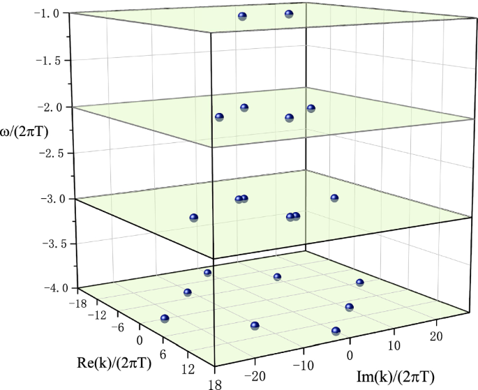
The pole-skipping points in acoustic black holes from Gross–Pitaeskii equation embedded in curved spacetime near acoustic horizon \(r_h=\sqrt{3}r_0\) (\(r_0=1\))
We expand the field equation near horizon \(r_h=\sqrt{3}r_0\). Now we repeat the process we have shown in Sect. 2 and calculate the special points \((\omega _n, k_n)\). The first three order pole-skipping points are in Fig. 4.
-
Case 2: near event horizon \({\varvec{r_0}}\) If we consider the pole-skipping points near the event horizon, Eq. (3.5) near the event horizon \(r=r_0\) by using \(f(r)\sim f'(r_0)(r-r_0)\) is
$$\begin{aligned} \psi ''(r)+(1-i{\mathfrak {w}})\frac{\psi '(r)}{r-r_0}-\frac{\pi T{\mathfrak {k}}^2+\sqrt{3}i{\mathfrak {w}}r_0^3}{\sqrt{3}r_0^4}\frac{\psi (r)}{r-r_0}=0. \end{aligned}$$(4.11)The first order special point is located at
$$\begin{aligned} {\mathfrak {w}}_{*}=-i,\quad {\mathfrak {k}}^{2}_{*}=-\frac{\sqrt{3}\, r_0^3}{\pi T}. \end{aligned}$$(4.12)

The location of the first three order pole-skipping points is shown in Fig. 5. These locations are also the poles of Green’s function that correspond to the hydrodynamic dispersion relation for momentum diffusion. The \({\mathfrak {k}}^{2}\) of the first order pole-skipping point near acoustic horizon to that near the event horizon is \({\mathfrak {k}}_{*h}^{2}/{\mathfrak {k}}_{*0}^{2}=r^3_h/r^3_0\). The data at these two horizons are only numerically different with which depend on \(r_h\) and \(r_0\). Combining with the first order pole-skipping points obtained above, we conclude that the frequency \({\mathfrak {w}}_{*}\) is always located at \(-i\). The square of momentum \({\mathfrak {k}}_{*}^{2}\) depends on the exponential power of the spatial metric value in the direction of momentum. For example, if the value of spatial metric \(d\phi ^2\) is \(r^m\), then the square of momentum \({\mathfrak {k}}_{*}^{2}\sim r_{h,0}^{m-1}/T\), where \(r_{h,0}\) is the acoustic and event horizon, respectively.

The pole-skipping points in acoustic black holes from Gross–Pitaeskii equation embedded in curved spacetime near event horizon \(r_0\) (\(r_0=1\))
5 Discussion and conclusion
We have shown the consistency between pole-skipping points and QNMs for Unruh’s acoustic black hole. Now we further conjecture that QNMs are consistent with the pole-skipping phenomenon in all cases of acoustic black holes. The analytic WKB approximations for QNMs are given as [42,43,44]
where n is the overtone number, \(\varOmega _c\) is the angular velocity at the unstable null geodesic, and l is the angular momentum of the perturbation. The notation \(\uplambda \) denotes the Lyapunov exponent. The real part of the complex QNM frequencies is found to be an integer multiple of the orbital angular frequency at the photon ring; the imaginary part is related to the Lyapunov exponent determining the unstable null orbits at the photon ring radius [45]. If we take the value of the maximal chaotic Lyapunov exponent as \(2\pi T\) near the black hole horizon, the imaginary part of QNMs becomes \(-i(n+1/2)2\pi T\). The coefficient of 1/2 plays the same role as 1/2 of the ground state in quantum mechanics. When we drop off this constant 1/2, the result is consistent with the frequencies of pole-skipping points (\(-in2\pi T\)) for acoustic black holes. So we can interpret the lower-half plane pole-skipping points in the acoustic black hole as some kind of dissipation of fluid perturbation.
In summary, we show that the pole-skipping phenomenon also exists in acoustic black holes. For acoustic black holes in Minkowski space, the existence of the pole-skipping indicates that it might be verified in the experiments. For acoustic black holes embedded in Schwarzschild black hole and AdS-Schwarzschild black hole, the existence of the pole-skipping implies its universality. For all cases, the frequencies \(\omega \) of these special points are the same as those black holes in gravity, which are located at negative integer (imaginary) Matsubara frequencies \({\mathfrak {w}}_{n}=-in\) \((n=1,2\dots )\). We conclude that the phenomenon of pole-skipping still exists in acoustic black holes, which are consistent with those in gravity.
We cannot obtain poles-skipping points by solving Green’s function directly without the boundary condition. Nevertheless, we have obtained the “pole-skipping” points by solving the bulk equations of motion near the horizon in Rindler geometry [15]. The procedure developed in [15] also applies to the acoustic black holes. For example, we calculate “pole-skipping” points in Eq. (2.19) near the acoustic horizon in Sect. 2. Two incoming waves (2.18) at these “pole-skipping” points correspond to the nonuniqueness of the Green’s function on the boundary. Combining with the previous conclusion in Rindler geometry, we conclude that the pole-skipping phenomenon does not depend on the UV property of the Green’s function.
We have shown that the frequencies of lower-half plane pole-skipping points in an acoustic black hole are the same as the imaginary frequencies of QNMs. This conclusion is consistent with our results in gravitational black holes [15]. This implies that the lower-half plane pole-skipping phenomenon has the same physical meaning as the imaginary of QNMs, which represents the dissipation of perturbation of acoustic black holes and is related to the decay timescale of the perturbation.
Data Availability Statement
This manuscript has no associated data or the data will not be deposited. [Authors’ comment: The main reason is that this paper is about theoretical study and almost all the steps are presented in the manuscript.]
References
S. Grozdanov, K. Schalm, V. Scopelliti, Phys. Rev. Lett. 120, 231601 (2018). arXiv:1710.00921
M. Blake, R.A. Davions, S. Grozdanov, H. Liu, JHEP 2018, 35 (2018). arXiv:1809.01169
S. Grozdanov, JHEP 2019, 48 (2019). arXiv:1811.09641
M. Natsuume, T. Okamura, and regularity, PTEP 2020, 013B07 (2020). arXiv:1905.12014
M. Natsuume, T. Okamura, arXiv:1905.12015
M. Blake, R.A. Davison, D. Vegh, JHEP 2020, 77 (2020). arXiv:1904.12883
M. Natsuume, T. Okamura, Phys. Rev. D 100, 126012 (2019). arXiv:1909.09168
S. Das, B. Ezhuthachan, A. Kundu, JHEP 2019, 141 (2019)
N. Abbasi, J. Tabatabaei, JHEP 2020, 50 (2020). arXiv:1910.13696
N. Abbasi, S. Tahery, JHEP 2020, 76 (2020). arXiv:2007.10024
Y. Ahn, V. Jahnke, H.S. Jeong, K.Y. Kim, K.S. Lee, M. Nishida, JHEP 2020, 111 (2020). arXiv:2006.00974
K.Y. Kim, K.S. Lee, M. Nishida, JHEP 2021, 20 (2021). arXiv:2105.07778
C. Choi, M. Mezei, G. Sárosi, JHEP 2021, 207 (2021). arXiv: 2010.08558
K. Sil, JHEP 2021, 232 (2021). arXiv:2012.07710
H. Yuan, X.H. Ge, JHEP 2021, 165 (2021). arXiv:2012.15396
W.G. Unruh, Phys. Rev. Lett. 46, 1351 (1981)
M. Visser, Classical Quantum Gravity 15, 1767 (1998). arXiv:gr-qc/9712010
C. Lan, Y.G. Miao, Y.X. Zang, arXiv:2109.13556
X.H. Ge, M. Nakahara, S.J. Sin, Y. Tian, S.F. Wu, Phys. Rev. D 99, 104047 (2019). arXiv:1902.11126
X.H. Ge, S.F. Wu, Y. Wang, G.H. Yang, Int. J. Mod. Phys. D 21, 1250038 (2012). arXiv:1010.4961
X.H. Ge, S.J. Sin, JHEP 2010, 87 (2010). arXiv:1001.0371
X.H. Ge, J.R. Sun, Y. Tian, X.N. Wu, Y.L. Zhang, Phys. Rev. D 92, 084052 (2015). arXiv:1508.01735
R. Ling, H. Guo, H. Liu, X.M. Kuang, B. Wang, arXiv:2107.05171
K.D. Kokkotas, B.G. Schmidt, Living Rev. Relativ. 2, 2 (1999). arXiv:gr-qc/9909058
E. Berti, V. Cardoso, A.O. Starinets, Class. Quantum Gravity 26, 163001 (2009). arXiv:0905.2975
Wenhe Cai, Xian-Hui. Ge, QingBing Wang, Phys. Rev. D 99, 106006 (2019). arXiv:1812.05258
F. Marino, Phys. Rev. A 78, 063804 (2008). arXiv:0808.1624
Y.S. Kivshar, G.P. Agrawal, Optical Solitons (Academic Press, London, 2003)
R.W. Boyd, Nonlinear Optics (Academic Press, London, 2008)
M. Ciszak, F. Marino, Phys. Rev. D 103, 045004 (2021)
N. Abbasi, M. Kaminski, JHEP 2021, 265 (2021). arXiv:2012.15820
H.S. Jeong, K.Y. Kim, Y.W. Sun, JHEP 2021, 105 (2021). arXiv:2104.13084
J. Saavedra, Mod. Phys. Lett. A 21, 1601 (2006). arXiv:gr-qc/0508040
L.D. Landau, E.M. Lifshitz, Fluid Mechanics (Pergamon Press, Oxford, 1993), p. p507
N. Bilic, Class. Quantum Gravity 16, 3953 (1999). arXiv:gr-qc/9908002
M. Visser, C. Molina-París, New J. Phys. 12, 095014 (2010). arXiv:1001.1310
V. Moncrief, Astrophys. J. 235, 1038 (1980)
Q.B. Wang, X.H. Ge, Phys. Rev. D 102, 104009 (2020). arXiv:1912.05285
E.P. Gross, Nuovo Cimento 20, 454 (1961)
L.P. Pitaevskii, Sov. Phys. JETP 13, 451 (1961)
S.A. Hartnoll, Class. Quantum Gravity 26, 224002 (2009). arXiv:0903.3246
B.F. Schutz, C.M. Will, Astrophys. J. 291, L33 (1985)
S. Iyer, C.M. Will, Phys. Rev. D 35, 3621 (1987)
V. Cardoso, A.S. Miranda, E. Berti, H. Witek, V.T. Zanchin, Phys. Rev. D 79, 064016 (2009). arXiv:0812.1806
K. Glampedakis, H.O. Silva, Phys. Rev. D 100, 04404. arXiv:1906.05455
Acknowledgements
We would like to thank Matteo Baggioli, Yu-Qi Lei, and Qing-Bing Wang for helpful discussions. This work is partly supported by NSFC (No. 11875184).
Author information
Authors and Affiliations
Corresponding author
Details of near-horizon expansions
Details of near-horizon expansions
In this appendix, we show the details of the near-horizon expansions of the equations of motion.
1.1 Acoustic black holes in Minkowski spacetime
We can calculate a Taylor series solution to the equation of field \(\psi (r)\) (2.15) when the matrix equation (2.23) is satisfied. The first few elements of this matrix are shown below
1.2 Acoustic black holes embedded in Schwarzschild spacetime
We can calculate a Taylor series solution to the equation of field \(\psi (r)\) (3.5) when the matrix equation (2.23) is satisfied. The first few elements of this matrix are
1.3 Acoustic black holes embedded in AdS-Schwarzschild spacetime
We can calculate a Taylor series solution to the equation of field \(\psi (r)\) (4.8) when the matrix equation (2.23) is satisfied. The first few elements of this matrix are (\(r_H\) is acoustic/event horizon)
Rights and permissions
Open Access This article is licensed under a Creative Commons Attribution 4.0 International License, which permits use, sharing, adaptation, distribution and reproduction in any medium or format, as long as you give appropriate credit to the original author(s) and the source, provide a link to the Creative Commons licence, and indicate if changes were made. The images or other third party material in this article are included in the article’s Creative Commons licence, unless indicated otherwise in a credit line to the material. If material is not included in the article’s Creative Commons licence and your intended use is not permitted by statutory regulation or exceeds the permitted use, you will need to obtain permission directly from the copyright holder. To view a copy of this licence, visit http://creativecommons.org/licenses/by/4.0/.
Funded by SCOAP3
About this article

Cite this article
Yuan, H., Ge, XH. Analogue of the pole-skipping phenomenon in acoustic black holes. Eur. Phys. J. C 82, 167 (2022). https://doi.org/10.1140/epjc/s10052-022-10129-y
Received:
Accepted:
Published:
DOI: https://doi.org/10.1140/epjc/s10052-022-10129-y