
Abstract
We calculate the weak decay form factors of doubly-heavy baryons using three-point QCD sum rules. The Cutkosky rules are used to derive the double dispersion relations. We include perturbative contributions and condensation contributions up to dimension five, and point out that the perturbative contributions and condensates with lowest dimensions dominate. An estimate of a part of the gluon–gluon condensates show that it plays a less important role. With these form factors at hand, we present a phenomenological study of semileptonic decays. The future experimental facilities can test these predictions, and deepen our understanding of the dynamics in the decays of doubly-heavy baryons.
1 Introduction
Although the quark model has achieved many brilliant successes in hadron spectroscopy, not all predicted particles, even in the ground state, in the quark model have been experimentally established so far. These states include doubly-heavy baryons and triply-heavy baryons. In 2017, the LHCb collaboration has reported the first observation of the doubly-charmed baryon \(\Xi _{cc}^{++}\) with the mass [1]
in the \(\Lambda _{c}^{+}K^{-}\pi ^{+}\pi ^{+}\) final state. Soon afterwards new results on \(\Xi _{cc}^{++}\) were released by LHCb, including the first measurement of its lifetime [2] and the observation of a new decay mode \(\Xi _{cc}^{++}\rightarrow \Xi _{c}^{+}\pi ^{+}\) [3]. On the experimental side, more investigations on \(\Xi _{cc}^{++}\) and searches for other doubly-heavy baryons are certainly required to achieve a better understanding [4, 5]. Meanwhile these observations have triggered many theoretical studies on various properties of doubly-heavy baryons [5,6,7,8,9,10,11,12,13,14,15,16,17,18,19,20,21,22,23,24,25,26,27,28,29,30,31,32,33,34,35,36,37,38,39,40,41,42], most of which have been focused on the spectrum, production and decay properties.
In a previous work [6], we have performed an analysis of the decay form factors of doubly-heavy baryons in a light-front quark model (LFQM). In this light-front study, the diquark picture is adopted, where the two spectator quarks are treated as a bounded system. This approximation can greatly simplify the calculation and many useful phenomenological results are obtained [28, 33]. Meanwhile this diquark approximation introduces uncontrollable systematic uncertainties since the dynamics in the diquark system has been smeared. In this work, we will remedy this shortcoming and perform an analysis of the transition form factors using QCD sum rules (QCDSRs). Some earlier attempts based on nonrelativistic QCD (NRQCD) sum rules can be found in Refs. [43,44,45]. It is necessary to note that, since the decay final state contains only one heavy quark, NRQCD should not be applicable unless the strange quark is also treated as a heavy quark. In the literature the QCDSR framework has also been used to calculate the masses and the pole residues of doubly-heavy baryons in a number of references (see for instance [18, 46,47,48,49]). So it is desirable to calculate the decay form factors within the same framework, which is the motif of this work.
In our analysis, the doubly-heavy baryons include \(\Xi _{cc}(ccq)\), \(\Omega _{cc}(ccs)\), \(\Xi _{bb}(bbq)\), \(\Omega _{bb}(bbs)\), and \(\Xi _{bc}(bcq)\), \(\Omega _{bc}(bcs)\), with \(q=u,d\). The \(\Xi _{QQ^{\prime }}\) and \(\Omega _{QQ^{\prime }}\) can form a flavor SU(3) triplet. It should be noted that the two heavy quarks in \(\Xi _{bc}\) and \(\Omega _{bc}\) are symmetric in the flavor space. The antisymmetric case, which presumably will decay via strong or electromagnetic interactions, are not considered in this work. Quantum numbers of doubly-heavy baryons can be found in Table 1. Baryons in the final state contain one heavy bottom/charm quark and two light quarks. They can form an SU(3) anti-triplet \(\Lambda _{Q}\), \(\Xi _{Q}\) or an SU(3) sextet \(\Sigma _{Q}\), \(\Xi _{Q}^{\prime }\) and \(\Omega _{Q}\) with \(Q=b,c\), as depicted in Fig. 1.

The anti-triplet (a) and sextet (b) of charmed baryons. It is similar for bottom baryons
To be more explicit, the transitions of doubly-heavy baryons can be classified as follows:
The cc sector
$$\begin{aligned} \Xi _{cc}\rightarrow & {} [\Lambda _{c},\Xi _{c},\Sigma _{c},\Xi _{c}^{\prime }], \;\;\; \Omega _{cc} \rightarrow [\Xi _{c},\Xi _{c}^{\prime }]. \end{aligned}$$The bb sector
$$\begin{aligned} \Xi _{bb}\rightarrow & {} [\Lambda _{b},\Sigma _{b}],\;\;\; \Omega _{bb} \rightarrow [\Xi _{b},\Xi _{b}^{\prime }]. \end{aligned}$$The bc sector with c quark decay
$$\begin{aligned} \Xi _{bc}\rightarrow & {} [\Lambda _{b},\Xi _{b},\Sigma _{b},\Xi _{b}^{\prime }],\;\;\; \Omega _{bc} \rightarrow [\Xi _{b},\Xi _{b}^{\prime }]. \end{aligned}$$The bc sector with b quark decay
$$\begin{aligned} \Xi _{bc}\rightarrow & {} [\Lambda _{c},\Sigma _{c}],\;\;\; \Omega _{bc} \rightarrow [\Xi _{c},\Xi _{c}^{\prime }]. \end{aligned}$$
In the above, both SU(3) anti-triplet and sextet final states are taken into account. However, the \(b\rightarrow c\) transition will not be considered in this work, and is left for the future.
The rest of this paper is arranged as follows. In Sect. 2, the transition form factors are calculated in QCDSR, where the perturbative contribution, quark condensates, quark–gluon condensates are calculated and an estimate of part of the gluon–gluon condensates is presented. Numerical results for the form factors are presented in Sect. 3, which are subsequently used to perform the phenomenological studies in Sect. 4. A brief summary of this work and the prospect for the future are given in the last section.

Feynman diagram for semileptonic decays. The leptonic amplitude can be calculated using perturbation theory, while hadronic matrix elements can be parametrized into form factors
2 Transition form factors in QCD sum rules
2.1 Form factors
We show the Feynman diagram for semileptonic decays of doubly-heavy baryons in Fig. 2. The leptonic amplitude in this transition can be calculated using electro-weak perturbation theory, while the hadronic matrix elements can be parametrized into transition form factors:
where \(p_1(s_1)\) is the momentum (spin) of the initial state, and \(p_2(s_2)\) is the momentum (spin) of the final baryon. The momentum transfer is defined as \(q^\mu = p_1^\mu -p_2^\mu \), and the vector (axial-vector) \(V^\mu (A^\mu )\) is defined as \({{\bar{q}}}_1' \gamma ^\mu (\gamma ^\mu \gamma ^5) Q_1\), with \(q_1'\) being a light quark and \(Q_1\) as a heavy bottom or charm quark. \(M_1\) is the mass of the initial doubly-heavy baryon. These form factors are also responsible for non-leptonic decay modes if the factorization holds, and thus must be calculated in a nonperturbative manner for later use.
In our calculation, the following simple parametrization will be used first:
Once the form factors \(F_{i}\) and \(G_{i}\) in Eq. (3) are obtained, they will be transformed into \(f_{i}\) and \(g_{i}\) in Eq. (2), which are used to compare with other work in the literature.
2.2 QCD sum rules
The starting point in QCDSR is to construct a suitable correlation function, and for the \(\mathcal{B}_{Q_{1}Q_{2}q_{3}}\rightarrow \mathcal{B}_{q_{1}^{\prime }Q_{2}q_{3}}\) transition, it is chosen as
Here the weak transition \(Q_{1}\rightarrow q_{1}^{\prime }\) stands for the \(c\rightarrow d/s\) or \(b\rightarrow u\) process. The \(Q_{2}=c/b\), \(q_{3}=u/d/s\) and \(V_\mu (A_{\mu })={\bar{q}}_{1}^{\prime }\gamma _{\mu }(\gamma _\mu \gamma _{5})Q_{1}\). The \(J_{\mathcal{B}_{q_{1}^{\prime }Q_{2}q_{3}}}\) and \(J_{\mathcal{B}_{Q_{1}Q_{2}q_{3}}}\) are the interpolating currents for singly and doubly-heavy baryons, respectively. For \(\Xi _{QQ}\) and \(\Omega _{QQ}\), they are used as follows:
where \(Q=b,c\) and \(q=u,d\). For \(\Xi _{bc}\) and \(\Omega _{bc}\) the interpolating currents are
where the b and c fields are chosen symmetric. The interpolating currents for singly-heavy baryons can be defined in a similar way. For the SU(3) anti-triplet they are
and for the SU(3) sextet they are
Similar definitions for the interpolating currents were adopted in Refs. [46, 47, 54], and some discussions can be found in Ref. [46].
The correlation function can be calculated at both hadron and QCD level. In the following, we will only present the extraction of the vector-current form factors, and the axial-vector-current form factors can be determined in a similar way. At hadron level, one can insert complete sets of the initial and final hadronic states into the correlation function and consider the contributions from positive- and negative-parity baryons simultaneously, then the correlation function can be written as

In Eq. (9), the ellipsis stands for the contribution from higher resonances and continuum spectra, \(M_{1(2)}^{+(-)}\) denotes the mass of the initial (final) positive (negative) parity baryons, and \(F_{1}^{-+}\) is the form factor \(F_{1}\) defined in Eq. (3) with the negative-parity final state and the positive-parity initial state, and so forth. To arrive at Eq. (9), we have adopted the pole residue definitions for positive- and negative-parity baryons,
and the following conventions for the form factors \(F_{i}^{\pm \pm }\):
In Eq. (10), \(J_{+}\) can be found in Eqs. (5)–(8), and \(\lambda _{+(-)}\) is the pole residue for the positive (negative) parity baryon.
At the QCD level, the correlation function can be evaluated using the operator product expansion (OPE), and expanded as a power of matrix elements of local operators in the deep Euclidean momentum region. This expansion is organized by the inverse of mass dimensions. The identity operator corresponds to the so-called perturbative term and higher dimensional operators are called the condensate terms. A detailed calculation of these contributions will be presented in the following subsections, including the perturbative contribution (dim-0), the quark condensate contribution (dim-3) and the mixed quark–gluon condensate contribution (dim-5). For practical use, it is convenient to express the correlation function as a double dispersion relation,
with \(\rho _{\mu }^{V,{\mathrm{QCD}}}(s_{1},s_{2},q^{2})\) being the spectral function, which can be obtained by applying Cutkosky cutting rules. Quark–hadron duality guarantees that results for correlation functions derived at hadron level and QCD level are equivalent. In particular, it is plausible to identify the spectral functions above threshold at the hadron level and QCD level. Under this assumption, the sum of the four pole terms in Eq. (9) should be equal to
where \(s_{1(2)}^{0}\) is the threshold parameter for the initial (final) baryon. \(\Pi _{\mu }^{V,\mathrm{pole}}\) can be formally written as
where, for latter convenience, we define

Then one can obtain these 12 form factors \(F_{i}^{\pm ,\pm }\) in Eq. (9) by comparing the corresponding coefficients of these 12 Dirac structures at hadronic and QCD levels. Especially, one can obtain the expressions for \(F_{i}^{++}\):
In practice, Borel transformations are usually adopted to improve the convergence in the quark–hadron duality and suppress the higher resonance and continuum contributions:
where \(\mathcal{B}A_{i}\equiv \mathcal{B}_{T_{1}^{2},T_{2}^{2}}A_{i}\) are doubly Borel transformed coefficients, and \(T_{1}^{2}\) and \(T_{2}^{2}\) are the Borel mass parameters.
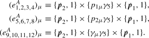
The coefficients \(A_{i}\) in Eq. (14) can be projected out in the following way. Multiplying by \(e_{j}^{\mu }\), then taking the trace on both sides of Eq. (14), one can arrive at the following 12 linear equations:
Solving these equations one can obtain these \(A_{i}\).
In the following, we will use the vector-current form factors for doubly-heavy baryon into a SU(3) sextet baryon as an example to illustrate our calculation. Results for other transitions can be obtained in a similar manner.

The perturbative contribution to transition form factors. The doubly-solid line denotes a heavy quark, and the ordinary solid line corresponds to a light quark
2.3 The perturbative contribution
The perturbative contribution is derived by computing the coefficient of the identity operator in OPE. The corresponding Feynman diagram is shown in Fig. 3. The doubly-solid line denotes a heavy bottom/charm quark, and the ordinary solid line corresponds to a light quark. Its contribution is given as
where the factor 6 comes from the color contraction \(\epsilon _{abc}\epsilon ^{abc}\), the factor \(2\sqrt{2}\) comes from the contraction of quark fields and the normalization factors of the baryon currents. The numerator of the integrand in Eq. (19) is

The correlation function can be expressed in terms of a double dispersion integration:
Here the spectral function \(\rho _{\mu }^{V,\mathrm{pert}}(s_{1},s_{2},q^{2})\) is proportional to the discontinuity of the correlation function with respect to \(s_{1}\) and \(s_{2}\). According to the Cutkosky rule, the spectral function can be obtained by setting all the propagators onshell:
The phase-space-like integral can be evaluated:
where
2.4 The quark condensate contribution
The \({{\bar{q}}} q\) condensate operator in the OPE has dimension 3, and its Feynman diagram is shown in Fig. 4. Since heavy quarks will not contribute with condensations, there are two diagrams from the light-quark condensate. The diagram (4a) gives
where the condensate term is defined as \(\langle q_{a}^{i}{\bar{q}}_{b}^{j}\rangle = - (\langle {\bar{q}}q\rangle /12)\delta _{ab}\delta ^{ij}\), and the numerator is


Light-quark condensate diagrams. The heavy quark will not condensate and thus only the two light-quark propagators give condensate contributions
According to the Cutkosky rule, the spectral function can now be evaluated as
where the integral \(\int _{\triangle }\) is slightly different from that in Eq. (24), with \(m_{23}^{2}\) being replaced by \(m_{2}^{2}\). The diagram (b) has the amplitude
One can see that the denominator is independent of \(p_{1}^{2}\), and thereby the corresponding double discontinuity must vanish. As a result, the quark condensate contribution only comes from Fig. 4a.
2.5 Mixed quark–gluon condensate contribution

Mixed quark–gluon condensate diagrams

Quark propagators in the QCD vaccum. x and y are spacetime coordinates, i and j are color indices, and \(p_{i}\), k and \(k_{i}\) are momenta
The quark–gluon condensate operator \({{\bar{q}}} g_s G q\) has dimension 5 in OPE. There are three Feynman diagrams for mixed quark–gluon condensate contribution, as shown in Fig. 5. We are required to consider the interaction of the propagating quark with the background gluons. The quark propagators with one gluon and two gluons attached (Fig. 6), respectively, have the following forms:

In the fixed-point gauge, the background gluon field expanded to the lowest order (in the momentum space) is
Thus a propagating quark can exchange arbitrary numbers of zero momentum gluons with the QCD vacuum. It should be noted that the fixed-point gauge violates the spacetime translation invariance. As a result, S(x, y) is not the same as \(S(x-y,0)\). In the cases of the quark–gluon condensate contribution and the gluon–gluon condensate contribution, to be discussed in the following, the following formulas are useful:

where u stands for the momentum of the soft gluon, and f(u) is an arbitrary function of u.
In Fig. 5a, the upper left heavy quark interacts with a background gluon field, which condensates with the two light-quark fields. Its contribution is given as
The condensate term is defined as \(\langle q^i_a g_s G^c_{\mu \nu } {{\bar{q}}}^j_b\rangle = -(1/192)\langle {\bar{q}} g_s \sigma G q\rangle (\sigma _{\mu \nu })^{ij}T^c_{ab}\), and the numerator is

In Eq. (31), \(1/(k_{1}^{2}-m_{1}^{2})^{3}\) can be handled by a derivative method:
Then the spectral function can be derived by using the Cutkosky rule before applying the mass derivative:
The integral \(\int _{\triangle }\) is slightly different from that in Eq. (27), with \(m_{1}^{2}\) being replaced by \(m_{1s}\). The other two diagrams in Fig. 5 can be calculated similarly.

One of the gluon–gluon condensate diagrams
2.6 Gluon–gluon condensate contribution
In the case of the dim-4 operator GG in the OPE, i.e. the gluon–gluon condensate, two background gluon fields interact with the four quark propagators, and one example is shown in Fig. 7.
The contribution from Fig. 7 is

Note that \(\Pi _{\mu }^{V,\langle GG\rangle }(p_{1}^{2},p_{2}^{2},q^{2})\) contains 19 Dirac matrices.
A similar procedure can be applied to extract the spectral function, and the corresponding numerical results will be shown in Sect. 3.
3 Numerical results
The input parameters used in our numerical calculation are taken as [50,51,52,53]: \(\langle {\bar{q}}q\rangle =-(0.24\pm 0.01{\mathrm{GeV}})^{3}\), \(\langle {\bar{s}}s\rangle =(0.8\pm 0.2)\langle {\bar{q}}q\rangle \), \(\langle {\bar{q}}g_{s}\sigma Gq\rangle =m_{0}^{2}\langle {\bar{q}}q\rangle \), \(\langle {\bar{s}}g_{s}\sigma Gs\rangle =m_{0}^{2}\langle {\bar{s}}s\rangle \), \(m_{0}^{2}=(0.8\pm 0.2)\ {\mathrm{GeV}}^{2}\), \(\langle \frac{\alpha _{s}GG}{\pi }\rangle =(0.012\pm 0.004)\ {\mathrm{GeV}}^{4}\) for the condensate parameters and \(m_{s}=(0.14\pm 0.01)\ {\mathrm{GeV}}\), \(m_{c}=(1.35\pm 0.10)\ {\mathrm{GeV}}\), \(m_{b}=(4.7\pm 0.1)\ {\mathrm{GeV}}\) for the quark masses. The pole residues of doubly-heavy and singly-heavy baryons as well as their masses are collected in Table 2. The factor \(\sqrt{2}\) in Table 2 arises from the convention difference in the definitions of the interpolating current for baryon [18, 54, 55]. For doubly-heavy baryons, we have updated the pole residues using the same inputs as those in this work. The mass of \(\Xi _{cc}^{++}\) comes from the experiment [1] and other masses of doubly-heavy baryons are predictions of the Lattice QCD [56]. The masses for baryons with a singly-heavy quark are taken from the Particle Data Group [52, 53]. The masses of the negative-parity baryons presented in Eq. (17) are collected in Table 3 [49, 57].
When arriving at the predictions of the branching ratios, the lifetimes of the initial doubly-heavy baryons are also needed. They are collected in Table 4, in which the lifetime of \(\Xi _{cc}^{++}\) comes from the experiment [2], and other results are the theoretical predictions [45, 58, 59].
The threshold parameters \(\sqrt{s_{1,2}^{0}}\) are taken from Table 2, which are essentially about 0.5 GeV higher than the corresponding baryon mass [60]. We employ the following equation from Ref. [61] to simplify the selection of the Borel mass parameters:
where \(M_{1(2)}\) is the mass of the initial (final) baryon and \(m_{1}^{(\prime )}\) is the mass of the initial (final) quark. To determine the window of the Borel parameter \(T_{1}^{2}\), the criteria of pole dominance,
and OPE convergence are invoked. For the latter, the reader can refer to Table 6. The obtained windows for \(T_{1}^{2}\) can be seen in Table 7. In Table 14, we have evaluated all the error sources for the form factors of \(\Xi _{cc}^{++}\rightarrow \Sigma _{c}^{+}\). One can see that the Borel parameter dependence is weak.
More comments on the selection of the Borel parameters are in order. \(T_{1}^{2}\) and \(T_{2}^{2}\) are in fact free parameters in the dispersion integral. To investigate the dependence on the Borel parameters, we take the \(\Xi _{cc}^{++}\rightarrow \Sigma _{c}^{+}\) process as an example. First, we calculate the form factors \(F_{1, 2, 3}(0)\) as functions of \(T_{1}^{2}\) and \(T_{2}^{2}\) in the square region [1, 10] \(\hbox {GeV}^{2}\times [1,10]\) \(\hbox {GeV}^{2}\). Then the obtained results are represented graphically in Fig. 8, where the positive and negative values are, respectively, displayed as reddish and bluish, and the greater the absolute value for the form factors \(F_{1, 2, 3}(0)\), the darker the color. In the end, the following three criteria are employed to determine the Borel region:
The pole dominance. See Eq. (36).
OPE convergence. This can be achieved by demanding that the contribution from the quark–gluon condensate (dim-5) is less than, for example, 10%.
Stability of the quantity within the Borel region. This can be read directly from Fig. 8.
More details can be found in Table 5. In Fig. 8, we also show the line segment determined by Eq. (35). It can be seen that the simplified equation (35) is still a good approximation, and a quantitative comparison between these two different ways to determine Borel parameters can be seen in Table 5.

\(F_{1, 2, 3}\) at \(q^{2}=0\) as functions of the Borel parameters \(T_{1}^{2}\) and \(T_{2}^{2}\) in the process of \(\Xi _{cc}^{++}\rightarrow \Sigma _{c}^{+}\), where \(T_{1}^{2}\) and \(T_{2}^{2}\) are taken as free parameters. Positive and negative values are, respectively, displayed as reddish (\(F_{1,2}\)) and bluish (\(F_{3}\)), and the greater the absolute value for the form factors \(F_{i}(0)\), the darker the color. The allowed Borel regions are enclosed by the dashed contours. To determine these regions, three criteria have been applied, as can be seen in the text. The red line segment determined by Eq. (35), which is adopted in this work, is also shown on each figure
Numerical results for the form factors are given in Tables 8, 9, 10 and 11 for the doubly-charmed, doubly-bottom and bottom–charm baryons. In QCDSR, the OPE is applicable in the deep Euclidean region, where \(q^{2}\ll 0\). In this work, we directly calculate the form factors in the region \(-\, 1<q^{2}<0\) \(\hbox {GeV}^{2}\) for the charm quark decay, and \(0<q^{2}<5\) \(\hbox {GeV}^{2}\) for the bottom quark decay. In order to access the \(q^{2}\) distribution in the full kinematic region, the form factors are extrapolated with a parametrization. We adopt the following double-pole parameterization:
A few remarks are given in order.
We have also calculated part of the gluon–gluon condensate, shown in Fig. 7, for \(\Xi _{cc}^{++}\rightarrow \Sigma _{c}^{+}\), and make a comparison with other contributions in Table 6. From this table, it is plausible to conclude to the following pattern:
$$\begin{aligned} \text {dim-0}\sim \text {dim-3}\gg \text {dim-5}\gg \text {dim-4}. \end{aligned}$$(38)We intend to perform a more comprehensive analysis by including all the contributions from the gluon–gluon condensate in the future.
The form factors \(g_{i}\) are determined in the following way. Rewrite Eq. (14) as
$$\begin{aligned} \Pi _{\mu }^{V,\mathrm{pole}}=\sum _{i=1}^{12}A_{i}^{V}e_{i\mu }^{V}, \end{aligned}$$(39)and similarly write the pole contribution for the axial-vector-current correlation function as
$$\begin{aligned} \Pi _{\mu }^{A,\mathrm{pole}}=\sum _{i=1}^{12}A_{i}^{A}e_{i\mu }^{A}, \end{aligned}$$(40)where \(e_{i\mu }^{V}\equiv e_{i\mu }\) in Eq. (15) and
 (41)
(41)In the massless limit \(m_{1}^{\prime }\rightarrow 0\) and \(m_{3}\rightarrow 0\), one can prove for the process of the final baryon belonging to the sextet:
$$\begin{aligned}&A_{i}^{A,\text {dim-0}}{=-}A_{i}^{V,\text {dim-0}},\,\, A_{i}^{A,\text {dim-3}}{=}A_{i}^{V,{\text {dim-3}}},\,\, A_{i}^{A,\text {dim-5}}{=}A_{i}^{V,\text {dim-5}},\,\,\text { for }i\text { odd},\nonumber \\&A_{i}^{A,{\text {dim-0}}}{=}A_{i}^{V,{\text {dim-0}}},\,\, A_{i}^{A,{\text {dim-3}}}{=-}A_{i}^{V,{\text {dim-3}}},\,\, A_{i}^{A,{\text {dim-5}}}{=-}A_{i}^{V,{\text {dim-5}}},\,\,\text { for }i\text { even},\nonumber \\ \end{aligned}$$(42)and for the process of the final baryon belonging to the anti-triplet:
$$\begin{aligned}&A_{i}^{A,\text {dim-0}}=A_{i}^{V,\text {dim-0}},\quad A_{i}^{A,\text {dim-3}}=-A_{i}^{V,{\text {dim-3}}},\quad A_{i}^{A,\text {dim-5}}=-A_{i}^{V,\text {dim-5}},\quad \text { for }i\text { odd},\nonumber \\&A_{i}^{A,{\text {dim-0}}}=-A_{i}^{V,{\text {dim-0}}},\quad A_{i}^{A,{\text {dim-3}}}=A_{i}^{V,{\text {dim-3}}},\quad A_{i}^{A,{\text {dim-5}}}=A_{i}^{V,{\text {dim-5}}},\quad \text { for }i\text { even}.\nonumber \\ \end{aligned}$$(43)Here \(A_{i}^{A,\text {dim-0}}\) stands for the coefficient \(A_{i}^{A}\) in Eq. (40) with the dim-0 correlation function being considered only, and so forth.
The uncertainties of form factors arise from those from the heavy quark masses, Borel parameter \(T_{1}^{2}\), thresholds \(s_{1}^{0}\) and \(s_{2}^{0}\), condensate parameters, pole residues and masses of initial and final baryons. A detailed analysis can be found in Sect. 3.1 and Table 14. It can be seen from 14 that the uncertainty mainly comes from that of the heavy quark mass. Thus, in Tables 8, 9, 10 and 11, we only list the uncertainties from the heavy quark masses.
In Table 8, the \(\Xi _{cc}\rightarrow \Sigma _{c}\) stands for the \(\Xi _{cc}^{++}\rightarrow \Sigma _{c}^{+}\) transition. A factor \(\sqrt{2}\) should be added for the \(\Xi _{cc}^{+}\rightarrow \Sigma _{c}^{0}\) transition. This is consistent with the analysis based on the flavor SU(3) symmetry [8]. Similar arguments can be found in Tables 9, 10, and 11.

A comparison between this work and other work in the literature can be found in Tables 12 and 13 for the cc sector, the bb sector and the bc sector with c or b quark decay.
Some comments:
The signs of the form factors of \(c\rightarrow d\) processes (\(\Xi _{cc}^{++}(ccu)\rightarrow \Lambda _{c}^{+}(dcu)\) and \(\Xi _{bc}^{+}(cbu)\rightarrow \Lambda _{b}^{0}(dbu)\)) in the LFQM have been flipped so that those of vector-current form factors are the same as ours. This stems from the asymmetry of u and d in the wave-function of \(\Lambda _{Q}=(1/\sqrt{2})(ud-du)Q\) with \(Q=c/b\) in the final state.
It can be seen from Tables 12 and 13 that most of our results are comparable with others in other literature up to a sign difference for the axial-vector-current form factors. However, this will not affect our predictions on physical observables; see Sect. 4.
The sign conventions for \(f_{2}\) and \(g_{2}\) in Refs. [62, 63] are different from ours in Eq. (2).
3.1 Uncertainties
In this subsection, we will investigate the dependence of the form factors on the inputs. \(\Xi _{cc}^{++}\rightarrow \Sigma _{c}^{+}\) is taken as an example. In Table 14, we have considered all the error sources including those from the heavy quark masses, Borel parameter \(T_{1}^{2}\), thresholds \(s_{1}^{0}\) and \(s_{2}^{0}\), condensate parameters, pole residues and masses of initial and final baryons. One can see that the uncertainty mainly comes from that of the heavy quark mass \(m_{c}\). That is, the results of the QCD sum rules are sensitive to the choice of the heavy quark mass. Similar situations are also encountered in studying other properties of heavy hadrons using QCD sum rules. In principle, this can be cured by calculating the contributions from the radiation corrections, which is undoubtedly a great challenge in the application of QCD sum rules. In this work, we will have to be content with the leading order results. Also note that the dependence of the form factors on the Borel parameter \(T_{1}^{2}\) is weak.
When all uncertainties are considered, from Table 14, the error estimates of the form factors at \(q^{2}=0\) for the \(\Xi _{cc}^{++}\rightarrow \Sigma _{c}^{+}\) transition turn out to be
4 Phenomenological applications
In this section, the results for the form factors will be applied to calculate the partial widths of semileptonic decays.
4.1 Semileptonic decays
The effective Hamiltonian for the semileptonic process reads
where \(G_{F}\) is the Fermi constant and \(V_{cs,cd,ub}\) are the Cabibbo–Kobayashi–Maskawa (CKM) matrix elements.
The helicity amplitudes will be used in the calculation and for the vector current and the axial-vector current, they are given as follows:
where \(Q_{\pm }=(M_1\pm M_2)^{2}-q^{2}\) and \(M_{1(2)}\) is the mass of the initial (final) baryon. The amplitudes for negative helicity are given by
where \(\lambda _{2}\) and \(\lambda _{W}\) denote the polarizations of the final baryon and the intermediate W boson, respectively. Then the helicity amplitudes for the \(V-A\) current are obtained:
The decay widths for \(\mathcal{B}_{1}\rightarrow \mathcal{B}_{2}l\nu \) with the longitudinally and transversely polarized \(l\nu \) pair are evaluated as
where \({\hat{m}}_{l}\equiv m_{l}/\sqrt{q^{2}}\), \(p=\sqrt{Q_{+}Q_{-}}/(2M_{1})\) is the magnitude of three-momentum of \(\mathcal{B}_{2}\) in the rest frame of \(\mathcal{B}_{1}\). Integrating out the squared momentum transfer \(q^{2}\), we obtain the total decay width:
where
The Fermi constant and CKM matrix elements are taken from the Particle Data Group [52, 53]:
The lifetimes of the doubly-heavy baryons are given in Table 4. The integrated partial decay widths, ratios of \(\Gamma _{L}/\Gamma _{T}\) and the corresponding branching fractions are calculated and the results are given in Tables 15, 16, 17 and 18, respectively. A comparison of our results with those in the literature is presented in Table 19.
A few remarks are given in order.
The \(c\rightarrow s\) induced channels like \(\Xi _{cc}^{++}\rightarrow \Xi _{c}^+l^+\nu _l\) have a large branching fraction, typically at a few percent level. This is comparable with the branching ratio of semileptonic D decays [52, 53].
To be compared with Ref. [6], in this work we have considered the contributions from the form factors \(f_{3}\) and \(g_{3}\).
In the flavor SU(3) limit, there exist the following relations for the charm quark decay widths:
$$\begin{aligned} \Gamma (\Xi _{cc}^{++}\rightarrow \Lambda _{c}^{+}l^{+}\nu )&=\Gamma (\Omega _{cc}^{+}\rightarrow \Xi _{c}^{0}l^{+}\nu ),\;\;\;\\ \Gamma (\Xi _{cc}^{++}\rightarrow \Xi _{c}^{+}l^{+}\nu )&=\Gamma (\Xi _{cc}^{+}\rightarrow \Xi _{c}^{0}l^{+}\nu ),\\ \Gamma (\Xi _{cc}^{++}\rightarrow \Sigma _{c}^{+}l^{+}\nu )&=\frac{1}{2}\Gamma (\Xi _{cc}^{+}\rightarrow \Sigma _{c}^{0}l^{+}\nu )=\Gamma (\Omega _{cc}^{+}\rightarrow \Xi _{c}^{\prime 0}l^{+}\nu ),\\ \Gamma (\Xi _{cc}^{++}\rightarrow \Xi _{c}^{\prime +}l^{+}\nu )&=\Gamma (\Xi _{cc}^{+}\rightarrow \Xi _{c}^{\prime 0}l^{+}\nu )=\frac{1}{2}\Gamma (\Omega _{cc}^{+}\rightarrow \Omega _{c}^{0}l^{+}\nu ),\\ \Gamma (\Xi _{bc}^{+}\rightarrow \Lambda _{b}^{0}l^{+}\nu )&=\Gamma (\Omega _{bc}^{0}\rightarrow \Xi _{b}^{-}l^{+}\nu ),\;\;\;\\ \Gamma (\Xi _{bc}^{+}\rightarrow \Xi _{b}^{0}l^{+}\nu )&=\Gamma (\Xi _{bc}^{0}\rightarrow \Xi _{b}^{-}l^{+}\nu ),\\ \Gamma (\Xi _{bc}^{+}\rightarrow \Sigma _{b}^{0}l^{+}\nu )&=\frac{1}{2}\Gamma (\Xi _{bc}^{0}\rightarrow \Sigma _{b}^{-}l^{+}\nu )=\Gamma (\Omega _{bc}^{0}\rightarrow \Xi _{b}^{\prime -}l^{+}\nu ),\\ \Gamma (\Xi _{bc}^{+}\rightarrow \Xi _{b}^{\prime 0}l^{+}\nu )&=\Gamma (\Xi _{bc}^{0}\rightarrow \Xi _{b}^{\prime -}l^{+}\nu )=\frac{1}{2}\Gamma (\Omega _{bc}^{0}\rightarrow \Omega _{b}^{-}l^{+}\nu ). \end{aligned}$$For the bottom quark decay, the relations for the decay widths are given as
$$\begin{aligned} \Gamma (\Xi _{bb}^{-}\rightarrow \Lambda _{b}^{0}l^{-}{\bar{\nu }})&=\Gamma (\Omega _{bb}^{-}\rightarrow \Xi _{b}^{0}l^{-}{\bar{\nu }}),\\ \Gamma (\Xi _{bb}^{0}\rightarrow \Sigma _{b}^{+}l^{-}{\bar{\nu }})&=2\Gamma (\Xi _{bb}^{-}\rightarrow \Sigma _{b}^{0}l^{-}{\bar{\nu }})=2\Gamma (\Omega _{bb}^{-}\rightarrow \Xi _{b}^{\prime 0}l^{-}{\bar{\nu }}), \\ \Gamma (\Xi _{bc}^{+}\rightarrow \Sigma _{c}^{++}l^{-}{\bar{\nu }})&=2\Gamma (\Xi _{bc}^{0}\rightarrow \Sigma _{c}^{+}l^{-}{\bar{\nu }})=2\Gamma (\Omega _{bc}^{0}\rightarrow \Xi _{c}^{\prime +}l^{-}{\bar{\nu }}). \end{aligned}$$Based on the results in Tables 15, 16, 17, and 18, we find that the SU(3) relations for some channels involving \(\Omega _{bc}\) and \(\Omega _{bb}\) are significantly broken.
In Tables 15, 16, 17, and 18, we have also shown the uncertainties for the phenomenological observables, which come from the uncertainties of the F(0) of the corresponding form factors. The latter uncertainties in turn come from those of the heavy quark masses. In Subsection 3.1, we have seen that the uncertainty from the heavy quark mass dominates.
It can be seen from Table 19 that most results in this work are comparable with those in the literature.
4.2 Dependence of decay width on the form factors
In this subsection, we will investigate the dependence of decay width on the form factors taking \(\Xi _{cc}^{++}\rightarrow \Sigma _{c}^{+}l^{+}\nu _{l}\) as an example. The uncertainties of the decay width caused by those of the form factors in Eq. (44) can be found in Table 20. One can see that these uncertainties are quite different; the largest one comes from that of \(g_{1}\). In fact, both \(f_{3}\) and \(g_{3}\) do not contribute to the decay width. This is because the leptonic part of the amplitude \({\bar{\nu }}\gamma _{\mu }(1-\gamma _{5})l\) when contracted with \(q^{\mu }\) from the hadronic matrix element vanishes if we neglect the masses of leptons. Finally, it is worth mentioning again that the uncertainty of \(g_{1}\) mainly comes from that of \(m_{c}\), as can be seen from Table 14.
The decay width turns out to be
Here we have only considered the uncertainties from the F(0), and we have also checked that those from \(m_{\mathrm{pole}}\) and \(\delta \) can be neglected. Note that here the uncertainties from the F(0) include those from the heavy quark mass \(m_{c}\), Borel parameter \(T_{1}^{2}\), thresholds \(s_{1}^{0}\) and \(s_{2}^{0}\), condensate parameters, pole residues and the masses of the initial and final baryons. If we only consider the uncertainty from the heavy quark mass \(m_{c}\) for the F(0), a slightly smaller error is obtained,
It can be seen that it is a good error estimate for the decay width if we only consider the uncertainties from the heavy quark masses. Thus, in Tables 15, 16, 17, and 18, only the uncertainties from the heavy quark masses are considered.
5 Conclusions
Since the observation of the doubly charmed baryon \(\Xi _{cc}^{++}\) reported by LHCb, many theoretical investigations have been triggered on the hadron spectroscopy and on the weak decays of the doubly-heavy baryons, most of which are based on phenomenological models rooted in QCD. In this work, we have presented a first QCD sum rules analysis of the form factors for the doubly-heavy baryon decays into singly-heavy baryon. We have included the perturbative contribution and condensation contributions up to dimension 5. We have also estimated the partial contributions from the gluon–gluon condensate, and found that these contributions are negligible. These form factors are then used to study the semileptonic decays. Future experimental measurements can examine these predictions and test the validity to apply QCDSR to doubly-heavy baryons.
With the advances of new LHCb measurements in the future and the experimental facilities under design, it is anticipated that more theoretical work of analyzing weak decays of doubly-heavy baryons will be conducted. In this direction, we can foresee the following prospects.
In this study, we have shown that part of the gluon–gluon condensate is small but an analysis with a complete estimate of gluon–gluon condensate is left for future.
The interpolating currents for the baryons are not uniquely determined. An ideal option is to have a largest projection onto the ground state of doubly-heavy baryons and to suppress the contributions from higher resonances and continuum. The dependence on interpolating current and an estimate of the corresponding uncertainties have to be conducted in a systematic way.
Decay form factors calculated in this work are induced by heavy to light transitions, and the heavy to heavy transition will be studied in the future. Another plausible framework is nonrelativistic QCD.
We have investigated the form factors defined by vector and axial-vector currents, while the tensor form factors are necessary to study the flavor-changing neutral current processes in bottom quark decays, like the radiative and the dilepton decay modes.
We have focused on the final baryons with spin-1/2, while the \(1/2\rightarrow 3/2\) transition needs an independent analysis.
Our calculation of the form factors is conducted at the leading order in the expansion of strong coupling constant. However, to achieve a more precise result, it is still necessary to perform the calculation of higher order radiative corrections in future work.
The ordinary QCD sum rules makes use of small-x OPE. In a heavy to light transition, there exists a large momentum transfer and it would be advantageous to adopt the light-cone OPE. Recently, the authors of Ref. [65] conducted the light-cone QCDSR study, and similar results are obtained.
Data Availability Statement
This manuscript has no associated data or the data will not be deposited. [Authors’ comment: There is no associated data in our paper.]
References
R. Aaij et al. [LHCb Collaboration], Phys. Rev. Lett. 119(11), 112001 (2017). https://doi.org/10.1103/PhysRevLett.119.112001. arXiv:1707.01621 [hep-ex]
R. Aaij et al. [LHCb Collaboration], Phys. Rev. Lett. 121(5), 052002 (2018). https://doi.org/10.1103/PhysRevLett.121.052002. arXiv:1806.02744 [hep-ex]
R. Aaij et al. [LHCb Collaboration], Phys. Rev. Lett. 121(16), 162002 (2018). https://doi.org/10.1103/PhysRevLett.121.162002. arXiv:1807.01919 [hep-ex]
M. T. Traill [LHCb Collaboration], PoS Hadron 2017, 067 (2018). https://doi.org/10.22323/1.310.0067
A. Cerri et al.,. arXiv:1812.07638 [hep-ph]
W. Wang, F.S. Yu, Z.X. Zhao, Eur. Phys. J. C 77(11), 781 (2017). https://doi.org/10.1140/epjc/s10052-017-5360-1. arXiv:1707.02834 [hep-ph]
L. Meng, N. Li, Sl Zhu, Eur. Phys. J. A 54(9), 143 (2018). https://doi.org/10.1140/epja/i2018-12578-2. arXiv:1707.03598 [hep-ph]
W. Wang, Z.P. Xing, J. Xu, Eur. Phys. J. C 77(11), 800 (2017). https://doi.org/10.1140/epjc/s10052-017-5363-y. arXiv:1707.06570 [hep-ph]
T. Gutsche, M.A. Ivanov, J.G. Körner, V.E. Lyubovitskij, Phys. Rev. D 96(5), 054013 (2017). https://doi.org/10.1103/PhysRevD.96.054013. arXiv:1708.00703 [hep-ph]
H.S. Li, L. Meng, Z.W. Liu, S.L. Zhu, Phys. Lett. B 777, 169 (2018). https://doi.org/10.1016/j.physletb.2017.12.031. arXiv:1708.03620 [hep-ph]
Z.H. Guo, Phys. Rev. D 96(7), 074004 (2017). https://doi.org/10.1103/PhysRevD.96.074004. arXiv:1708.04145 [hep-ph]
Q.F. Lü, K.L. Wang, L.Y. Xiao, X.H. Zhong, Phys. Rev. D 96(11), 114006 (2017). https://doi.org/10.1103/PhysRevD.96.114006. arXiv:1708.04468 [hep-ph]
L.Y. Xiao, K.L. Wang, Q.F. Lu, X.H. Zhong, S.L. Zhu, Phys. Rev. D 96(9), 094005 (2017). https://doi.org/10.1103/PhysRevD.96.094005. arXiv:1708.04384 [hep-ph]
N. Sharma, R. Dhir, Phys. Rev. D 96(11), 113006 (2017). https://doi.org/10.1103/PhysRevD.96.113006. arXiv:1709.08217 [hep-ph]
Y.L. Ma, M. Harada, J. Phys. G 45(7), 075006 (2018). https://doi.org/10.1088/1361-6471/aac86e. arXiv:1709.09746 [hep-ph]
F.S. Yu, H.Y. Jiang, R.H. Li, C.D. Lü, W. Wang, Z.X. Zhao, Chin. Phys. C 42(5), 051001 (2018). https://doi.org/10.1088/1674-1137/42/5/051001. arXiv:1703.09086 [hep-ph]
L. Meng, H.S. Li, Z.W. Liu, S.L. Zhu, Eur. Phys. J. C 77(12), 869 (2017). https://doi.org/10.1140/epjc/s10052-017-5447-8. arXiv:1710.08283 [hep-ph]
X.H. Hu, Y.L. Shen, W. Wang, Z.X. Zhao, Chin. Phys. C 42(12), 123102 (2018). https://doi.org/10.1088/1674-1137/42/12/123102. arXiv:1711.10289 [hep-ph]
E.L. Cui, H.X. Chen, W. Chen, X. Liu, S.L. Zhu, Phys. Rev. D 97(3), 034018 (2018). https://doi.org/10.1103/PhysRevD.97.034018. arXiv:1712.03615 [hep-ph]
Y.J. Shi, W. Wang, Y. Xing, J. Xu, Eur. Phys. J. C 78(1), 56 (2018). https://doi.org/10.1140/epjc/s10052-018-5532-7. arXiv:1712.03830 [hep-ph]
L.Y. Xiao, Q.F. Lü, S.L. Zhu, Phys. Rev. D 97(7), 074005 (2018). https://doi.org/10.1103/PhysRevD.97.074005. arXiv:1712.07295 [hep-ph]
X. Yao, B. Müller, Phys. Rev. D 97(7), 074003 (2018). https://doi.org/10.1103/PhysRevD.97.074003. arXiv:1801.02652 [hep-ph]
D.L. Yao, Phys. Rev. D 97(3), 034012 (2018). https://doi.org/10.1103/PhysRevD.97.034012. arXiv:1801.09462 [hep-ph]
U. Özdem, J. Phys. G 46(3), 035003 (2019). https://doi.org/10.1088/1361-6471/aafffc. arXiv:1804.10921 [hep-ph]
A. Ali, A.Y. Parkhomenko, Q. Qin, W. Wang, Phys. Lett. B 782, 412 (2018). https://doi.org/10.1016/j.physletb.2018.05.055. arXiv:1805.02535 [hep-ph]
J.M. Dias, V.R. Debastiani, J.-J. Xie, E. Oset, Phys. Rev. D 98(9), 094017 (2018). https://doi.org/10.1103/PhysRevD.98.094017. arXiv:1805.03286 [hep-ph]
R.H. Li, C.D. Lu,. arXiv:1805.09064 [hep-ph]
Z.X. Zhao, Eur. Phys. J. C 78(9), 756 (2018). https://doi.org/10.1140/epjc/s10052-018-6213-2. arXiv:1805.10878 [hep-ph]
Y. Xing, R. Zhu, Phys. Rev. D 98(5), 053005 (2018). https://doi.org/10.1103/PhysRevD.98.053005. arXiv:1806.01659 [hep-ph]
R. Zhu, X.L. Han, Y. Ma, Z.J. Xiao, Eur. Phys. J. C 78, 740 (2018). https://doi.org/10.1140/epjc/s10052-018-6214-1. arXiv:1806.06388 [hep-ph]
A. Ali, Q. Qin, W. Wang, Phys. Lett. B 785, 605 (2018). https://doi.org/10.1016/j.physletb.2018.09.018. arXiv:1806.09288 [hep-ph]
M.Z. Liu, Y. Xiao, L.S. Geng, Phys. Rev. D 98(1), 014040 (2018). https://doi.org/10.1103/PhysRevD.98.014040. arXiv:1807.00912 [hep-ph]
Z.P. Xing, Z.X. Zhao, Phys. Rev. D 98(5), 056002 (2018). https://doi.org/10.1103/PhysRevD.98.056002. arXiv:1807.03101 [hep-ph]
R. Aaij et al. [LHCb Collaboration], arXiv:1808.08865
W. Wang, R. Zhu,. arXiv:1808.10830 [hep-ph]
R. Dhir, N. Sharma, Eur. Phys. J. C 78(9), 743 (2018). https://doi.org/10.1140/epjc/s10052-018-6220-3
A.V. Berezhnoy, A.K. Likhoded, A.V. Luchinsky, Phys. Rev. D 98(11), 113004 (2018). https://doi.org/10.1103/PhysRevD.98.113004. arXiv:1809.10058 [hep-ph]
L.J. Jiang, B. He, R.H. Li, Eur. Phys. J. C 78(11), 961 (2018). https://doi.org/10.1140/epjc/s10052-018-6445-1. arXiv:1810.00541 [hep-ph]
Q.A. Zhang, Eur. Phys. J. C 78(12), 1024 (2018). https://doi.org/10.1140/epjc/s10052-018-6481-x. arXiv:1811.02199 [hep-ph]
G. Li, X.F. Wang, Y. Xing, Eur. Phys. J. C 79(3), 210 (2019). https://doi.org/10.1140/epjc/s10052-019-6729-0. arXiv:1811.03849 [hep-ph]
L. Meng, S.L. Zhu, Phys. Rev. D 100(1), 014006 (2019). https://doi.org/10.1103/PhysRevD.100.014006. arXiv:1811.07320 [hep-ph]
T. Gutsche, M.A. Ivanov, J.G. Körner, V.E. Lyubovitskij, Z. Tyulemissov, Phys. Rev. D 99(5), 056013 (2019). https://doi.org/10.1103/PhysRevD.99.056013. arXiv:1812.09212 [hep-ph]
A. I. Onishchenko. arXiv:hep-ph/0006271
A. I. Onishchenko. arXiv:hep-ph/0006295
V. V. Kiselev, A. K. Likhoded, Phys. Usp. 45, 455 (2002) [Usp. Fiz. Nauk 172, 497 (2002)] https://doi.org/10.1070/PU2002v045n05ABEH000958[hep-ph/0103169]
J.R. Zhang, M.Q. Huang, Phys. Rev. D 78, 094007 (2008). https://doi.org/10.1103/PhysRevD.78.094007. arXiv:0810.5396 [hep-ph]
Z.G. Wang, Eur. Phys. J. A 45, 267 (2010). https://doi.org/10.1140/epja/i2010-11004-3. arXiv:1001.4693 [hep-ph]
Z.G. Wang, Eur. Phys. J. C 68, 459 (2010). https://doi.org/10.1140/epjc/s10052-010-1357-8. arXiv:1002.2471 [hep-ph]
Z.G. Wang, Eur. Phys. J. A 47, 81 (2011). https://doi.org/10.1140/epja/i2011-11081-8. arXiv:1003.2838 [hep-ph]
B.L. Ioffe, Prog. Part. Nucl. Phys. 56, 232 (2006). https://doi.org/10.1016/j.ppnp.2005.05.001. arXiv:hep-ph/0502148
P. Colangelo and A. Khodjamirian, In *Shifman, M. (ed.): At the frontier of particle physics, vol. 3* 1495-1576 https://doi.org/10.1142/9789812810458_0033. arXiv:hep-ph/0010175]
C. Patrignani et al. [Particle Data Group], Chin. Phys. C 40, no. 10, 100001 (2016). https://doi.org/10.1088/1674-1137/40/10/100001
M. Tanabashi et al. [Particle Data Group], Phys. Rev. D 98, no. 3, 030001 (2018). https://doi.org/10.1103/PhysRevD.98.030001
Z.G. Wang, Eur. Phys. J. C 68, 479 (2010). https://doi.org/10.1140/epjc/s10052-010-1365-8. arXiv:1001.1652 [hep-ph]
Z.G. Wang, Phys. Lett. B 685, 59 (2010). https://doi.org/10.1016/j.physletb.2010.01.039. arXiv:0912.1648 [hep-ph]
Z.S. Brown, W. Detmold, S. Meinel, K. Orginos, Phys. Rev. D 90(9), 094507 (2014). https://doi.org/10.1103/PhysRevD.90.094507. arXiv:1409.0497 [hep-lat]
W. Roberts, M. Pervin, Int. J. Mod. Phys. A 23, 2817 (2008). https://doi.org/10.1142/S0217751X08041219. arXiv:0711.2492 [nucl-th]
M. Karliner, J.L. Rosner, Phys. Rev. D 90(9), 094007 (2014). https://doi.org/10.1103/PhysRevD.90.094007. arXiv:1408.5877 [hep-ph]
H.Y. Cheng, Y.L. Shi, Phys. Rev. D 98(11), 113005 (2018). https://doi.org/10.1103/PhysRevD.98.113005. arXiv:1809.08102 [hep-ph]
Z.G. Wang, Eur. Phys. J. A 49, 131 (2013). https://doi.org/10.1140/epja/i2013-13131-7. arXiv:1203.6252 [hep-ph]
P. Ball, V.M. Braun, H.G. Dosch, Phys. Rev. D 44, 3567 (1991). https://doi.org/10.1103/PhysRevD.44.3567
R. Perez-Marcial, R. Huerta, A. Garcia, M. Avila-Aoki, Phys. Rev. D 40, 2955 (1989) Erratum: [Phys. Rev. D 44, 2203 (1991)]. https://doi.org/10.1103/PhysRevD.44.2203, https://doi.org/10.1103/PhysRevD.40.2955
L.J. Carson, R.J. Oakes, C.R. Willcox, Phys. Rev. D 33, 1356 (1986). https://doi.org/10.1103/PhysRevD.33.1356
C. Albertus, E. Hernandez, J. Nieves, PoS QNP 2012, 073 (2012). https://doi.org/10.22323/1.157.0073. arXiv:1206.5612 [hep-ph]
Y.J. Shi, Y. Xing, Z.X. Zhao, Eur. Phys. J. C 79(6), 501 (2019). https://doi.org/10.1140/epjc/s10052-019-7014-y. arXiv:1903.03921 [hep-ph]
Acknowledgements
The authors are grateful to Hai-Yang Cheng, Pietro Colangelo, Jürgen Körner, Run-Hui Li, Yu-Ming Wang, Zhi-Gang Wang, Fan-Rong Xu, Mao-Zhi Yang, Fu-Sheng Yu for useful discussions. This work is supported in part by National Natural Science Foundation of China under Grants No.11575110, 11735010,11911530088, Natural Science Foundation of Shanghai under Grants No. 15DZ2272100, and by Key Laboratory for Particle Physics, Astrophysics and Cosmology, Ministry of Education.
Author information
Authors and Affiliations
Corresponding authors
Rights and permissions
Open Access This article is licensed under a Creative Commons Attribution 4.0 International License, which permits use, sharing, adaptation, distribution and reproduction in any medium or format, as long as you give appropriate credit to the original author(s) and the source, provide a link to the Creative Commons licence, and indicate if changes were made. The images or other third party material in this article are included in the article’s Creative Commons licence, unless indicated otherwise in a credit line to the material. If material is not included in the article’s Creative Commons licence and your intended use is not permitted by statutory regulation or exceeds the permitted use, you will need to obtain permission directly from the copyright holder. To view a copy of this licence, visit http://creativecommons.org/licenses/by/4.0/.
Funded by SCOAP3
About this article

Cite this article
Shi, YJ., Wang, W. & Zhao, ZX. QCD Sum Rules Analysis of Weak Decays of Doubly-Heavy Baryons. Eur. Phys. J. C 80, 568 (2020). https://doi.org/10.1140/epjc/s10052-020-8096-2
Received:
Accepted:
Published:
DOI: https://doi.org/10.1140/epjc/s10052-020-8096-2