Non-perturbative determination of improvement coefficients $b_\mathrm{m}$ and $b_\mathrm{A}-b_\mathrm{P}$ and normalisation factor $Z_\mathrm{m}Z_\mathrm{P}/Z_\mathrm{A}$ with $N_\mathrm{f}= 3$ Wilson fermions

Abstract

We determine non-perturbatively the normalisation parameter $Z_\mathrm{m}Z_\mathrm{P}/Z_\mathrm{A}$ as well as the Symanzik coefficients $b_\mathrm{m}$ and $b_\mathrm{A}-b_\mathrm{P}$, required in $\mathrm{O}(a)$ improved quark mass renormalisation with Wilson fermions. The strategy underlying their computation involves simulations in $N_\mathrm{f}=3$ QCD with $\mathrm{O}(a)$ improved massless sea and non-degenerate valence quarks in the finite-volume Schrödinger functional scheme. Our results, which cover the typical gauge coupling range of large-volume $N_\mathrm{f}=2+1$ QCD simulations with Wilson fermions at lattice spacings below $0.1\,\mathrm{fm}$, are of particular use for the non-perturbative calculation of $\mathrm{O}(a)$ improved renormalised quark masses.

1 Introduction

Quark masses are amongst the fundamental parameters of the theory of strong interactions. Their high-precision determination is one of the main goals of lattice QCD (see Ref. [1] and references therein). These computations suffer from statistical and systematic uncertainties, which can be reduced in a controlled way. An important source of uncertainty are cutoff effects, which are removed by computing a given quantity at several lattice spacings, followed by continuum extrapolation. For several variants of lattice fermions (staggered, domain wall, overlap, twisted-mass) these uncertainties are ${\mathrm{O}}(a^2)$, while for Wilson fermions they are ${\mathrm{O}}(a)$. A related problem in the latter formulation is the loss of chiral symmetry, because it complicates the renormalisation properties of most quantities. A frequently cited example of these complications is the power divergence $m_{\mathrm{crit}} \sim 1/a$ that must be subtracted from bare quark masses before they are renormalised multiplicatively. Another example is the fact that the normalisation factor $Z_{\mathrm{A}}$ of the axial current and the ratio $Z_{\mathrm{S}}/Z_{\mathrm{P}}$ of the scalar and pseudoscalar density renormalisation parameters are finite functions of the gauge coupling, which are equal to unity only in the continuum limit where chiral symmetry is fully recovered.

In spite of these shortcomings, Wilson fermions have advantages compared to other popular regularisations, namely strict locality (leading to relatively reduced computational costs) and preservation of flavour symmetry. It is the regularisation of choice of our collaboration, which is part of the effort by the CLS (Coordinated Lattice Simulations) cooperation to simulate QCD with $N_\mathrm{f}=2+1$ flavours of non-perturbatively improved Wilson fermions [2,3,4,5].

Wilson fermion ${\mathrm{O}}(a)$ discretisation effects are systematically removed by introducing so-called Symanzik counter-terms in the lattice action and composite operators. These counter-terms are higher dimensional operators with coefficients which are functions of the gauge coupling. The coefficients must be appropriately tuned so that ${\mathrm{O}}(a)$ improvement is achieved. Some of them ($c_\mathrm{sw}, c_\mathrm{A}$, etc.) remove discretisation effects which are present also in the chiral limit, whereas others ($b_\mathrm{m}, b_\mathrm{A}, b_\mathrm{P}$, etc.) are proportional to the quark masses and improve quantities off the chiral limit. The requirement for improvement in the fermionic sector has been noted early on [6], and only a few strategies to determine them non-perturbatively have been developed so far.

In the present work we compute non-perturbatively the coefficients $b_\mathrm{m}$, $b_\mathrm{A}- b_\mathrm{P}$ and the renormalisation parameter $Z\equiv Z_\mathrm{m} Z_{\mathrm{P}}/Z_{\mathrm{A}}$ in a theory of three sea quark flavours. The methods we use can be traced back to Ref. [7]. In that work, renormalised quark masses were defined both through the PCAC bare quark masses and the subtracted bare Wilson masses. In both definitions ${\mathrm{O}}(a)$ improvement is introduced through the inclusion of all necessary c- and b-type counter-terms. Combining these results at constant bare gauge coupling provides estimates of $b_\mathrm{m}$, $b_\mathrm{A}- b_\mathrm{P}$ and Z. This work has been extended in Refs. [8,9,10], where results for other improvement coefficients were also reported. These computations were performed in large volumes with (anti)periodic boundary conditions. In parallel, in Ref. [11] (and subsequently in [12]) the method was extended and applied to small physical volumes with Schrödinger functional boundary conditions. These early analyses were carried out in the quenched approximation. More recently, in Ref. [13], $b_\mathrm{m}$, ${b_\mathrm{A}-b_\mathrm{P}}$ and Z were measured in a theory with $N_\mathrm{f}=2$ sea quarks, employing the Schrödinger functional scheme and working at a constant value of the renormalised coupling, so as to keep the physical extent of the lattice fixed. By thus imposing improvement and renormalisation conditions along a line in lattice parameter space, where all physical scales stay constant, it is ensured that any intrinsic higher-order lattice spacing ambiguities of b-coefficients and Z-factors vanish uniformly as the continuum limit is approached.

Our strategy follows closely that of Ref. [13]. However, the extraction of the final estimates from our data has been improved by the introduction of several novelties in the data analysis, which enable us to obtain very reliable estimates in the chiral limit. The lattice action we employ consists of the tree-level Symanzik-improved gauge action [14] and the non-perturbatively improved Wilson-clover fermion action [15]. Our simulations are performed in the range of bare couplings, where gauge configurations on lattices with large physical volumes with $N_\mathrm{f}=2+1$ sea quarks have been generated by CLS [2, 4]. These configurations are suitable for the computation of bare correlation functions, on the basis of which low-energy hadronic quantities can be evaluated. In Ref. [3] bare PCAC quark masses have been computed from these ensembles. To obtain renormalised up, down, and strange quark masses from these bare masses, one also needs the following: (i) The multiplicative mass renormalisation factor $1/Z_{\mathrm{P}}$ at low energies and its non-perturbative running up to high energy scales; these are known in the Schrödinger functional scheme from Ref. [16]. (ii) The axial current improvement coefficient $c_{\mathrm{A}}$ and its normalisation constant $Z_{\mathrm{A}}$, which are known from Refs. [17,18,19], respectively. (iii) The improvement coefficient $b_\mathrm{A}-b_\mathrm{P}$, which is one of the results of this work. (iv) The improvement coefficient ${\bar{b}}_{\mathrm{A}}-\bar{b}_{\mathrm{P}}$, which is particularly difficult to estimate but may be ignored, as it is sub-leading in perturbation theory.

Independent estimates of Symanzik b-coefficients, directly computed on CLS ensembles and obtained with a variant of the coordinate space method of Ref. [20], have been reported in [21]. A comparison of these results to ours may be found in Sect. 5. Preliminary results of the present work have been reported in Ref. [22]. For recent determinations of b-coefficients in the vector channel of three-flavour QCD with the same lattice action, see also Refs. [23, 24].

2 Quark mass renormalisation and improvement with Wilson fermions

In this section we review the renormalisation and ${\mathrm{O}} (a)$ improvement of quark masses in the framework of lattice regularisation with Wilson quarks. These results were first derived in Ref. [25] for QCD with degenerate masses and generalised in Ref. [26], which is the basis of our résumé. The starting point is the subtracted bare quark mass of flavour i ($i=1, \ldots , N_\mathrm{f}$),

$$\begin{aligned} m_{\mathrm{q},i}\equiv m_{0,i} - m_{\mathrm{crit}}&= \dfrac{1}{2a} \left( \dfrac{1}{\kappa _i}-\dfrac{1}{\kappa _{\mathrm{crit}}} \right) , \end{aligned}$$

(2.1)

where $\kappa _i$ is the hopping parameter, $\kappa _{\mathrm{crit}}$ its critical value corresponding to the chiral limit with $N_\mathrm{f}$ degenerate flavours, and a is the lattice spacing. In terms of the subtracted masses $m_{\mathrm{q},i}$, the ${\mathrm{O}}(a)$ improved, renormalised quark mass is given by

$$\begin{aligned} m_{i,\mathrm R}&= Z_\mathrm{m}\left\{ \left[ \, m_{\mathrm{q},i}+ (r_{\mathrm{m}} - 1)\frac{\mathrm {Tr}{[}M_\mathrm{q}{]}}{N_\mathrm{f}} \,\right] + a B_{i} \right\} + {\mathrm{O}}(a^2), \nonumber \\ B_{i}&= b_\mathrm{m}m_{\mathrm{q},i}^2 + {\bar{b}}_{\mathrm{m}} m_{\mathrm{q},i}\mathrm {Tr}{[}M_\mathrm{q}{]} + (r_{\mathrm{m}} d_{\mathrm{m}} - b_\mathrm{m}) \dfrac{\mathrm {Tr}{[}M_\mathrm{q}^2{]}}{N_\mathrm{f}} \nonumber \\&\quad + (r_{\mathrm{m}} {\bar{d}}_{\mathrm{m}} - {\bar{b}}_{\mathrm{m}}) \dfrac{\mathrm {Tr}{[}M_\mathrm{q}{]}^2}{N_\mathrm{f}}, \end{aligned}$$

(2.2)

where $M_\mathrm{q}= \mathrm{diag}(m_{\mathrm{q},1}, \ldots , m_{\mathrm{q},N_\mathrm{f}})$ is the $N_\mathrm{f}\times N_\mathrm{f}$ bare mass matrix (of subtracted quark masses), and $B_{i}$ a combination of Symanzik counter-terms cancelling ${\mathrm{O}}(a)$ mass-dependent cutoff effects. The $\mathrm {Tr}{[}M_\mathrm{q}{]}$-term in the square brackets appears at leading order and represents a redefinition of the chiral point in the presence of massive quarks.

We recall in passing that the renormalisation parameter $Z_\mathrm {m}(g_0^2,a\mu )$ depends on the renormalisation scale $\mu$ and diverges logarithmically in the ultraviolet. A mass-independent renormalisation scheme is implied throughout this work. In such a scheme, the Symanzik coefficients $b_\mathrm{m}$, $\bar{b}_{\mathrm{m}}$, $d_{\mathrm{m}}$, ${\bar{d}}_{\mathrm{m}}$ as well as $r_{\mathrm{m}}$ are functions of the squared bare coupling $g_0^2$.¹ In a non-perturbative determination at non-zero quark mass, they are affected by ${\mathrm{O}}(am_{\mathrm{q},i})$ and ${\mathrm{O}}(a\mathrm {Tr}{[}M_\mathrm{q}{]})$ systematic effects, which are part of their operational definition. They have the following properties:²

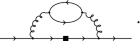
• (i) The $(r_{\mathrm{m}}-1)$-term multiplies $\mathrm {Tr}{[}M_\mathrm{q}{]}$, so it arises from a mass insertion on a quark loop; i.e., from diagrams like

  

  where the filled square indicates a mass insertion. It is a two-loop effect, contributing at ${\mathrm{O}}(g_0^4)$. Its determination is beyond the scope of this paper.

• (ii) The $b_\mathrm{m}$-term multiplies $m_{\mathrm{q},i}^2$. Thus it arises from: (a) the mass dependence of valence quark propagators and (b) the mass-independent contributions of the fermion loops. The former dependence begins at tree-level, so that $b_\mathrm {m}=-1/2+{\mathrm{O}}(g_0^2)$, corresponding to Feynman diagrams like

  

  The latter dependence begins at two loops, contributing at ${\mathrm{O}}( g_0^4)$; cf. for example diagram

  

  The quenched $b_\mathrm{m}$-value differs from the one of the full $N_\mathrm{f}$ theory by the mass-independent contributions of the fermion loops; consequently the difference arises at two loops and is ${\mathrm{O}}( g_0^4)$.

• (iii) The ${\bar{b}}_{\mathrm{m}}$-term multiplies $m_{\mathrm{q},i}\mathrm {Tr}{[}M_\mathrm{q}{]}$. The factor of $m_{\mathrm{q},i}$ comes from the valence line, while the $\mathrm {Tr}{[}M_\mathrm{q}{]}$ from a quark loop. It thus begins at two loops in perturbation theory (${\bar{b}}_{\mathrm{m}} \sim {\mathrm{O}}( g_0^4)$) and vanishes in the quenched approximation; e.g., diagram

  

  The determination of the ${\bar{b}}_{\mathrm{m}}$-term is beyond the scope of this paper.

• (iv) The $(r_{\mathrm{m}} d_{\mathrm{m}} - b_\mathrm{m})$-term multiplies $\mathrm {Tr}{[}M_\mathrm{q}^2{]}$; so it must arise from two insertions of $m_{\mathrm{q},i}$ on a single sea-quark loop. This combination begins at two loops, so it is ${\mathrm{O}}( g_0^4)$; cf. diagram

  

  But since it arises from sea quark propagators, while $b_\mathrm{m}$ has tree-level and ${\mathrm{O}}( g_0^2)$ valence-quark contributions, it follows that also $d_{\mathrm{m}}$ must get tree-level contributions and ${\mathrm{O}}( g_0^2)$ corrections from valence lines. The determination of $(r_{\mathrm{m}} d_{\mathrm{m}} - b_\mathrm{m})$ is beyond the scope of this paper.

• (v) The $(r_{\mathrm{m}} {\bar{d}}_{\mathrm{m}} - {\bar{b}}_{\mathrm{m}})$-term multiplies $\mathrm {Tr}{[}M_\mathrm{q}{]}^2$, so it can only arise from mass insertions on two separate quark loops. Thus this term begins at three loops and is ${\mathrm{O}}( g_0^6)$; cf. diagram

  

  But since ${\bar{b}}_{\mathrm{m}}$ itself begins at two loops, so must $\bar{d}_{\mathrm{m}}$. The determination of $(r_{\mathrm{m}} {\bar{d}}_{\mathrm{m}} - \bar{b}_{\mathrm{m}})$ is beyond the scope of this paper.

Next we recall that with Wilson fermions the renormalised quark mass can also be related to the bare PCAC mass $m_{ij}$, defined through the following relation:

$$\begin{aligned} (\partial _\mu )_x\big \langle (A_{\mathrm{I}})^{ij}_\mu (x)\,{\mathcal {O}}^{ji}\big \rangle \,=\, 2\,m_{ij} \, {\big \langle {P}^{ij}(x)\,{\mathcal {O}}^{ji}\big \rangle }, \end{aligned}$$

(2.3)

where $m_{ij} = \left( m_{i}+m_{j}\right) /2$. Our notation is standard: the non-singlet bare axial current and the pseudoscalar density are given by

$$\begin{aligned}&A_{\mu }^{ij}(x) \,\equiv \, \overline{\psi }_i(x)\,\gamma _{\mu }\gamma _{5}\,\psi _j(x),\nonumber \\&P^{ij}(x) \,\equiv \, \overline{\psi }_i(x)\,\gamma _{5}\,\psi _j(x), \end{aligned}$$

(2.4)

with indices i, j denoting two distinct flavours. The pseudoscalar density $P^{ij}$ and the current $(A_{\mathrm{I}})^{ij}_\mu \equiv A^{ij}_\mu +ac_\mathrm{A}\partial _\mu P^{ij}$ are Symanzik-improved in the chiral limit, with the improvement coefficient $c_\mathrm{A}(g_0^2)$ being in principle only a function of the gauge coupling.³

The operator ${\mathcal {O}}^{ji}$ is defined in a region of space-time that does not include the point x, thus avoiding contact terms. Our specific choice of correlation functions for Eq. (2.3) is discussed in Appendix B.

Beyond the chiral limit, composite operators require improvement through the introduction of b-type Symanzik counter-terms. The renormalised and ${\mathrm{O}}(a)$ improved axial current and pseudoscalar density are given by [25, 26]

$$\begin{aligned} (A_{\mathrm{R}})_{\mu }^{ij}(x)&= Z_\mathrm{A}(g_0^2)\left[ \,1+b_\mathrm{A}(g_0^2)\,a m_{\mathrm{q},ij} \right. \nonumber \\&\quad \left. +\, {\bar{b}}_{\mathrm{A}}(g_0^2)\,a \mathrm {Tr}{[}M_\mathrm{q}{]} \,\right] (A_\mathrm{I})_{\mu }^{ij}(x), \end{aligned}$$

(2.5)

$$\begin{aligned} (P_{\mathrm{R}})^{ij}(x)&= Z_\mathrm{P}(g_0^2,a\mu )\left[ \,1+b_\mathrm{P}(g_0^2) \,a m_{\mathrm{q},ij} \right. \nonumber \\&\quad \left. +\, {\bar{b}}_{\mathrm{P}}(g_0^2)\,a \mathrm {Tr}{[}M_\mathrm{q}{]} \, \,\right] P^{ij}(x), \end{aligned}$$

(2.6)

with $m_{\mathrm{q},ij} \equiv \left( m_{\mathrm{q},i}+m_{\mathrm{q},j}\right) /2$. The normalisation of the axial current $Z_\mathrm {A}(g_0^2)$ is scale-independent, depending only on the squared gauge coupling $g_0^2$. The renormalisation parameter $Z_\mathrm {P}(g_0^2,a\mu )$ also depends on the renormalisation scale $\mu$ and diverges logarithmically in the ultraviolet. The Symanzik coefficients $b_\mathrm{A}$, $b_\mathrm{P}$, ${\bar{b}}_{\mathrm{A}}$ and ${\bar{b}}_{\mathrm{P}}$ are in principle only functions of the bare squared coupling. They have the following properties:

• (vi) The $b_\mathrm{A}$- and $b_\mathrm{P}$-terms multiply $m_{\mathrm{q},ij}$. Thus they arise from: (a) the mass dependence of valence quark propagators and (b) the mass-independent contributions of the fermion loops. The former dependence begins at tree-level, so that $b_\mathrm{A}, b_\mathrm{P}\, = \, 1/2 + {\mathrm{O}}( g_0^2)$; cf. diagrams

  

  The latter dependence begins at two loops, contributing at ${\mathrm{O}}( g_0^4)$; cf. diagram

  

  The difference $b_\mathrm{A}- b_\mathrm{P}$, appearing in Eq. (2.8) below, is therefore ${\mathrm{O}}( g_0^2)$. The quenched values differ from those of the full $N_\mathrm{f}$ theory by the mass-independent contributions of the fermion loops; consequently the difference arises at two loops and is ${\mathrm{O}}( g_0^4)$.

• (vii) The ${\bar{b}}_{\mathrm{A}}$- and ${\bar{b}}_{\mathrm{P}}$-terms multiply $\mathrm {Tr}{[}M_\mathrm{q}{]}$. They arise from the mass dependence of quark fermion loops. They begin at two loops in perturbation theory (${\bar{b}}_\mathrm{A}, {\bar{b}}_{\mathrm{P}} \sim {\mathrm{O}}( g_0^4)$) and vanish in the quenched approximation; cf. diagram

  

  The determination of these coefficients is beyond the scope of this paper.

The renormalised PCAC relation

$$\begin{aligned}&\big \langle \, \partial _\mu (A_{\mathrm{R}})^{ij}_\mu (x)\ {\mathcal {O}}^{ji}\, \big \rangle \nonumber \\&= (m_{\mathrm{R},i}+m_{\mathrm{R},j})\,\big \langle \, (P_\mathrm {R})^{ij}(x)\ {\mathcal {O}}^{ji}\,\big \rangle +\mathrm{O}(a^2), \end{aligned}$$

(2.7)

valid up to ${\mathrm{O}}(a^2)$ effects, combined with Eqs. (2.3)–(2.6), implies that

$$\begin{aligned} \dfrac{m_{i,\mathrm R} + m_{j,\mathrm R}}{2}= & {} \dfrac{Z_\mathrm{A}}{Z_\mathrm{P}} \, m_{ij} \Big [\, 1 \, + \, (b_\mathrm{A}-b_\mathrm{P}) a m_{\mathrm{q},ij} \, \nonumber \\&+ \, (\bar{b}_{\mathrm{A}} - {\bar{b}}_{\mathrm{P}})a \mathrm {Tr}{[}M_\mathrm{q}{]} \,\Big ] \,+\, {\mathrm{O}}(a^2) \,\,. \end{aligned}$$

(2.8)

The properties of the various b-coefficients listed above Eqs. (2.2), (2.5), (2.6) and (2.8) also apply to the non-unitary theory, where valence and sea quarks of the same flavour have different masses. We saw that all terms containing traces of the fermion matrix refer to sea quarks, while the others refer to valence quarks. This is shown somewhat more explicitly in Appendix A. The present and previous works, such as Ref. [13], rely on this property in order to obtain reliable non-perturbative estimates of the Symanzik coefficients $b_\mathrm{m}$ and $b_\mathrm{A}-b_\mathrm{P}$, as well as the combination

$$\begin{aligned} Z \,\equiv \, Z_\mathrm{m}\,\frac{ Z_{\mathrm{P}}}{Z_{\mathrm{A}}}. \end{aligned}$$

(2.9)

2.1 Non-perturbative determination of $b_\mathrm{m}$, $b_\mathrm{A}-b_\mathrm{P}$ and Z

If we calculate the average mass $(m_{i,\mathrm R} + m_{j,\mathrm R})/2$ from Eq. (2.2) and equate the result to the r.h.s. of Eq. (2.8), we obtain an expression, which relates subtracted and PCAC bare masses:

$$\begin{aligned} m_{ij}&= \dfrac{Z_\mathrm{m}Z_\mathrm{P}}{Z_\mathrm{A}} \left\{ \left[ \, m_{\mathrm{q},ij} + (r_\mathrm{m}-1) \dfrac{\mathrm {Tr}{[}M_\mathrm{q}{]}}{N_\mathrm{f}} \,\right] + aB_{ij} \,\right\} + {\mathrm{O}}(a^2), \nonumber \\ B_{ij }&= b_\mathrm{m}\frac{m_{\mathrm{q},i}^2+m_{\mathrm{q},j}^2}{2} - (b_\mathrm{A}-b_\mathrm{P})m_{\mathrm{q},ij}^2 \nonumber \\&\quad + \Big ( {\bar{b}}_{\mathrm{m}} - (b_\mathrm{A}-b_\mathrm{P}) \dfrac{(r_\mathrm{m}-1)}{N_\mathrm{f}} - ({\bar{b}}_{\mathrm{A}} - {\bar{b}}_{\mathrm{P}}) \Big ) m_{\mathrm{q},ij} \mathrm {Tr}{[}M_\mathrm{q}{]} \nonumber \\&\quad + (r_{\mathrm{m}} d_{\mathrm{m}} - b_\mathrm{m}) \dfrac{\mathrm {Tr}{[}M_\mathrm{q}^2{]}}{N_\mathrm{f}} \nonumber \\&\quad + \Big ( (r_{\mathrm{m}} {\bar{d}}_{\mathrm{m}} - {\bar{b}}_{\mathrm{m}}) - (r_{\mathrm{m}}-1) ({\bar{b}}_{\mathrm{A}} - {\bar{b}}_{\mathrm{P}}) \Big ) \dfrac{\mathrm {Tr}{[}M_\mathrm{q}{]}^2}{N_\mathrm{f}}.\nonumber \\ \end{aligned}$$

(2.10)

Note that the product of the renormalisation parameters $Z_\mathrm {P}(g_0^2,\mu ) Z_\mathrm {m}(g_0^2,\mu )$ is scale independent.

As discussed previously and in Appendix A, Eq. (2.10) remains valid in the non-unitary theory, with $m_{\mathrm{q},i}$ denoting valence quark masses and $M_\mathrm{q}$ the mass matrix of sea quarks. Since $b_\mathrm{A}-b_\mathrm{P}$, $b_\mathrm{m}$ and the combination $Z \equiv Z_\mathrm{m}Z_{\mathrm{P}}/Z_{\mathrm{A}}$ are short distance quantities, they can be determined in small physical volumes with Schrödinger functional boundary conditions. This allows for simulations with degenerate sea quarks lying very close to the chiral limit, so that terms containing $\mathrm {Tr}{[}M_\mathrm{q}{]}$ can be dropped in Eq. (2.10). Following the strategy already proposed in Refs. [11, 13], we introduce two valence quark flavours with subtracted masses $m_{\mathrm{q},1} < m_{\mathrm{q},2}$ and their average $m_{\mathrm{q},3} \equiv (m_{\mathrm{q},1} +m_{\mathrm{q},2})/2$. It is then straightforward to obtain estimators of the desired improvement coefficients and normalisation factor Z from the ratios

$$\begin{aligned} R_\mathrm{AP}&\equiv \dfrac{2\left( 2m_{12}-m_{11}-m_{22}\right) }{\left( m_{11}-m_{22}\right) \left( am_{\mathrm{q},1}-am_{\mathrm{q},2}\right) }\nonumber \\&= (b_\mathrm{A}-b_{\mathrm{P}})\big \{ 1+\mathrm{O}\big (am_{\mathrm{q},12}; a \mathrm {Tr}{[}M_\mathrm{q}{]} \big )\big \}, \end{aligned}$$

(2.11a)

$$\begin{aligned} R_\mathrm{m}&\equiv \dfrac{4\left( m_{12}-m_{33}\right) }{\left( m_{11}-m_{22}\right) \left( am_{\mathrm{q},1}-am_{\mathrm{q},2}\right) } \nonumber \\&= b_\mathrm{m}\big \{ 1+\mathrm{O}\big (am_{\mathrm{q},12} ; a \mathrm {Tr}{[}M_\mathrm{q}{]} \big )\big \}, \end{aligned}$$

(2.11b)

$$\begin{aligned} R_{Z}&\equiv \dfrac{m_{11}-m_{22}}{m_{\mathrm{q},1}-m_{\mathrm{q},2}} +\left( R_\mathrm{AP}-R_\mathrm{m}\right) \left( am_{11}+am_{22}\right) \nonumber \\&= Z \big \{ 1 + \mathrm{O}\big (a^2; a \mathrm {Tr}{[}M_\mathrm{q}{]}\big ) \big \}, \end{aligned}$$

(2.11c)

where bare PCAC masses $m_{ii}$ (with $i=1,2,3$) are defined through Eq. (2.3) for two degenerate but distinct flavours.

Note that the leading improvement coefficients obtained from $R_\mathrm{AP}$ and $R_\mathrm{m}$ suffer from mass-dependent $\mathrm{O}(a)$ effects, which introduce only ${\mathrm{O}}(a^2)$ uncertainties in the quark masses; cf. Eqs. (2.2) and (2.8). The $\mathrm{O}(a \mathrm {Tr}{[}M_\mathrm{q}{]})$ effects appearing on the r.h.s. of Eqs. (2.11a), (2.11b) and (2.11c) arise from the presence of a residual non-zero sea quark mass in realistic simulations. This uncertainty is removed once simulations are performed for several sea quark masses and the chiral limit is reached by extrapolation. In our setup we are also able to simulate negative current quark masses, so in practice interpolation to the chiral limit is also possible. In the chiral limit, the leading normalisation factor Z of the estimator $R_Z$ suffers from $\mathrm{O}\big (a^2\big )$ effects; this is easily derived from Eqs. (2.10) and (2.11c).

The above ratios are not the only possible estimators of the quantities of interest. For example, we can modify $R_\mathrm{AP}$ and $R_\mathrm{m}$ by replacing the denominator $\left( m_{11}-m_{22}\right)$ by any of the following PCAC mass differences: $2(m_{22}-m_{33})$, $2(m_{33}-m_{11})$, $2(m_{22}-m_{12})$, or $2 (m_{12}-m_{11})$. As shown in Ref. [22], these new ratios also provide estimates of $(b_\mathrm{A}- b_\mathrm{P})$, $b_\mathrm{m}$ and Z, with different finite cutoff effects. In practice these differences were found to be orders of magnitude smaller than other systematic effects. So we have retained the original estimators $R_\mathrm{AP}$, $R_\mathrm{m}$ and $R_{Z}$ in the present work.

As previously stated, improvement coefficients are short distance quantities, which can be determined in small physical volumes, using the Schrödinger functional setup, with $L^3 \times T$ lattices having periodic boundary conditions in space and Dirichlet boundary conditions in time. Definitions of boundary operators and related correlation functions are given in Appendix B. For reasons explained above, sea quark masses are tuned closely to the chiral limit, in line with the usual ALPHA Collaboration choice of mass-independent renormalisation schemes.

2.2 The strategy revisited

In Refs. [11, 13] the computation of the Symanzik b-coefficients proceeds as follows: the PCAC quark masses $m_{11}$, $m_{22}$, $m_{12}$ and $m_{33}$ are first determined in standard fashion from Eq. (B.3), and are subsequently fed into the ratios $R_X$ (with $X=\mathrm{AP}, \mathrm{m}, Z$) defined in Eqs. (2.11a), (2.11b) and (2.11c). In some cases, this procedure turns out to suffer from numerical instabilities: the numerators of $R_X$ are current quark mass differences, i.e., constructed so that the leading contributions in powers of the lattice spacing a cancel, isolating the b-counter-terms. If these delicate cancellations in the mass differences occur with inadequate precision, the signal may be lost to the noise. Moreover, as we decrease the heavier quark mass $m_{\mathrm{q},2}$ towards $m_{\mathrm{q},1}$, striving to reduce discretisation effects, both numerator and denominator of the three estimators $R_X$ will contrive to give a noisy signal. We will show in Appendix C (cf. Fig. 10) examples of this instability. In order to overcome this problem, we introduce here a more elaborate method of analysis of quark masses evaluated from correlator measurements, which should ameliorate the stability of the results.

We start with some general considerations. At fixed gauge coupling, the bare PCAC quark masses $m_{ij}$ defined in Eq. (2.3) depend on the subtracted valence quark masses $m_{\mathrm{q},i}$ and $m_{\mathrm{q},j}$ and the trace of the sea quark mass matrix $\mathrm {Tr}{[}M_\mathrm{q}{]}$. Since in our simulations sea quark masses are very close to the chiral limit but not strictly zero, in what follows we keep $\mathrm {Tr}{[}M_\mathrm{q}{]}$ terms in the equations. The current masses $m_{ij}$ are symmetric functions under the exchange $m_{\mathrm{q},i} \leftrightarrow m_{\mathrm{q},j}$. This implies that they can be expressed as a power series of the form

$$\begin{aligned} am_{ij}( am_{\mathrm{q},ij}, a\Delta _{ij} )= \sum _{n,k=0}^\infty C_{nk} (a\Delta _{ij})^{2n} (am_{\mathrm{q},ij})^k, \end{aligned}$$

(2.12)

with the mass-splitting denoted as $\Delta _{ij}\equiv \tfrac{1}{2}(m_{\mathrm{q},i}-m_{\mathrm{q},j})$ and the dimensionless coefficients as $C_{nk}$. The latter only depend on the gauge coupling and flavour-blind traces of the sea quark masses.

To next-to-leading order in the lattice spacing, the Symanzik expansion for this expression is given by Eq. (2.10). A comparison with Eq. (2.12) shows that, to this order, the expansion coefficients read

$$\begin{aligned} C_{00}&= Z \,\dfrac{a\mathrm {Tr}{[}M_\mathrm{q}{]}}{N_\mathrm{f}} \Bigg \{ (r_{\mathrm{m}}-1) + (r_{\mathrm{m}} d_{\mathrm{m}} - b_\mathrm{m}) \dfrac{a\mathrm {Tr}{[}M_\mathrm{q}^2{]}}{\mathrm {Tr}{[}M_\mathrm{q}{]}}\nonumber \\&\quad + \Big ( (r_{\mathrm{m}} {\bar{d}}_\mathrm{m} - {\bar{b}}_{\mathrm{m}}) - (r_{\mathrm{m}}-1) ({\bar{b}}_{\mathrm{A}} - {\bar{b}}_{\mathrm{P}}) \Big ) a\mathrm {Tr}{[}M_\mathrm{q}{]} \Bigg \} \;, \end{aligned}$$

(2.13a)

$$\begin{aligned} C_{01}&= Z \,\Big \{ 1+ \Big ( {\bar{b}}_{\mathrm{m}} - ({\bar{b}}_{\mathrm{A}}- {\bar{b}}_{\mathrm{P}}) \nonumber \\&\quad - (b_\mathrm{A}-b_\mathrm{P}) {(r_{\mathrm{m}}-1)}/{N_\mathrm{f}} \Big ) a\mathrm {Tr}{[}M_\mathrm{q}{]} \Big \} \;, \end{aligned}$$

(2.13b)

$$\begin{aligned} C_{02}&= Z \,\Big \{ b_\mathrm{m}- (b_\mathrm{A}- b_\mathrm{P}) \Big \} \;, \end{aligned}$$

(2.13c)

$$\begin{aligned} C_{10}&= Z \,b_\mathrm{m}. \end{aligned}$$

(2.13d)

If the sea quark masses were tuned exactly to their critical value, we would have $C_{00} = 0$ and $C_{01} = Z$. Moreover, all $C_{nk}$ would be functions of only $g_0^2$ in perturbation theory. A non-perturbative determination of the $C_{nk}$, however, depends on the imposed improvement condition.

Turning next to the specific case under study, we recall that the ratios $R_{X}$ require three quark masses. We define the lightest one to be $m_{\mathrm{q},1}$ and set it to the value of the three degenerate sea quark masses used in our simulations, thus having $m_{\mathrm{q},1}=\mathrm {Tr}{[}M_\mathrm{q}{]}/N_\mathrm{f}$. In practice, its value is very small, but not strictly zero within statistical errors, cf. the x-axis of Fig. 3. The heavier mass is $m_{\mathrm{q},2}$ and the average of the two is $m_{\mathrm{q},3}$, i.e., we have $m_{\mathrm{q},2}> m_{\mathrm{q},3} > m_{\mathrm{q},1}$. Starting from Eq. (2.12), we now write the current quark masses $m_{11}, m_{22}$ and $m_{12}$ as power series, with $m_{22}$ and $m_{12}$ re-expressed in terms of $m_{\mathrm{q},1}$ and the (partially-quenched) mass-splitting $\Delta \equiv \tfrac{1}{2}(m_{\mathrm{q},2} - m_{\mathrm{q},1}) = m_{\mathrm{q},3} - m_{\mathrm{q},1}$:

$$\begin{aligned} am_{11}&= \sum _{k=0}^\infty C_{0k} (am_{\mathrm{q, 1}})^k, \end{aligned}$$

(2.14)

$$\begin{aligned} am_{22}(\Delta )&= \sum _{k=0}^\infty C_{0k} (am_{\mathrm{q, 1}} + 2a\Delta )^k, \end{aligned}$$

(2.15)

$$\begin{aligned} am_{12}(\Delta )&= \sum _{n,k=0}^\infty C_{nk} (a\Delta )^{2n} \big ( am_{\mathrm{q},1}+ a\Delta \big )^k. \end{aligned}$$

(2.16)

We observe that their first derivatives are exactly related via

$$\begin{aligned} \frac{1}{2}\frac{\partial m_{22}}{\partial \Delta }\bigg |_{\Delta =0} = \frac{\partial m_{12}}{\partial \Delta }\bigg |_{\Delta =0} = \frac{\partial m_{11}}{\partial m_{\mathrm{q},1}} . \end{aligned}$$

(2.17)

By construction, the unitary setup is recovered when $\Delta \rightarrow 0$, in which case ${m_{12},m_{22}\rightarrow m_{11}}$. Written in this way, we can always expand the masses $am_{12}$ and $am_{22}$ close to $am_{11}$, where then $\Delta$ becomes the expansion parameter:

$$\begin{aligned} am_{12}(\Delta )&= am_{11} + N_1 a\Delta + N_2 (a\Delta )^2 + \mathrm{O}(\Delta ^3), \end{aligned}$$

(2.18)

$$\begin{aligned} am_{22}(\Delta )&= am_{11} + 2 N_1 a\Delta + 4 D_2 (a\Delta )^2 + \mathrm{O}(\Delta ^3). \end{aligned}$$

(2.19)

The coefficients $N_i$ and $D_i$ for the flavour non-diagonal and diagonal masses, respectively, are linear combinations of the $C_{nk}$ and carry a residual dependence on $am_{\mathrm{q},1}$. Our particular choice of the third mass, $m_{\mathrm{q},3}\equiv m_{\mathrm{q},12}$, leads to the identity $m_{33}(\Delta )\equiv m_{22}(\Delta /2)$. Accordingly, we have the expansion

$$\begin{aligned} am_{33}(\Delta )&= am_{11} + N_1 a\Delta + D_2(a\Delta )^2 + \mathrm{O}(\Delta ^3) \end{aligned}$$

(2.20)

at our disposal and can revisit Eq. (2.11) in the context of our current discussion:

$$\begin{aligned} R_{\mathrm{AP}}&\equiv \dfrac{2 m_{12} - m_{11} - m_{22}}{(m_{22} - m_{11})\,a\Delta } \nonumber \\&= \dfrac{ N_2 - 2D_2 + \mathrm{O}(a\Delta )}{N_1+ \mathrm{O}(a\Delta )} \quad \xrightarrow {\Delta ,m_{\mathrm{q},1} \rightarrow 0} \quad b_\mathrm{A}-b_\mathrm{P}, \end{aligned}$$

(2.21a)

$$\begin{aligned} R_\mathrm{m}&\equiv \dfrac{2\left( m_{12}-m_{33}\right) }{\left( m_{22}-m_{11}\right) \,a\Delta } \nonumber \\&= \dfrac{ N_2 - D_2+ \mathrm{O}(a\Delta )}{ N_1+ \mathrm{O}(a\Delta )}\quad \xrightarrow {\Delta ,m_{\mathrm{q},1} \rightarrow 0} \quad b_\mathrm{m}, \end{aligned}$$

(2.21b)

$$\begin{aligned} R_Z&\equiv \dfrac{m_{22}-m_{11}}{2\Delta } + [R_\mathrm{AP}-R_\mathrm{m}](am_{11}+am_{22}) \nonumber \\&= N_1 - \frac{2 D_2 am_{11}}{{N_1}} + \mathrm{O}\big ((a\Delta )^2\big ) \quad \xrightarrow {\Delta ,m_{\mathrm{q},1} \rightarrow 0} \quad Z. \end{aligned}$$

(2.21c)

The original estimator $R_Z$ was constructed in order to cancel an $\mathrm{O}(a\Delta )$ effect [11], i.e., to reduce the largest bias in the determination of the leading order factor Z. In the unquenched theory, uncancelled $\mathrm{O}(a\mathrm {Tr}{[}M_\mathrm{q}{]})$ effects remain in all quantities. They are typically supressed by 1–2 orders in magnitude due to the sea quark mass tuning ($m_{11}\approx 0$) required in a mass-independent renormalisation scheme. In the determination of the estimators $R_X$, a renormalised trajectory, or line of constant physics (LCP), has to be employed such that they adopt the proper scaling behaviour when the bare gauge coupling $g_0^2$ is varied. This means that, besides $m_{11}=0$, a value for the mass-splitting $\Delta$, which fixes the LCP in the valence sector, has to be specified. In principle, any sensible choice $\Delta \ne 0$ is sufficient to define a valid set $\{R_\mathrm{AP},R_{\mathrm{m}},R_{Z}\}_\Delta$ that achieves $\mathrm{O}(a)$ improvement in physical quantities. Different choices lead to somewhat different approaches to the continuum limit and are equivalent in the framework of Symanzik’s effective theory. Their relative difference is a higher-order cutoff effect that vanishes for $a\rightarrow 0$ as can be easily seen in Eq. (2.21). A non-perturbative determination of these estimators inherits a non-trivial all-order dependence on $a\Delta$ if the limit $\Delta \rightarrow 0$ is not taken. In that sense, an explicit choice of $\Delta$ constitutes an ambiguity in their definition. In Ref. [13], for instance, $\Delta$ has been held constant by requiring $Lm_{22}\approx 0.5$ at constant physical L with $L/a\in [12,24]$.

In the present paper we aim at eliminating this $\Delta$-ambiguity in the definition of $R_{\mathrm{AP}}$, $R_{\mathrm{m}}$ and $R_{Z}$, because it can potentially lead to larger cutoff effects in the physics of light quarks. By noting that Eqs. (2.18) and (2.19) for $am_{ij}$ can literally be used as joint ansatz for interpolating fit functions (polynomials in $a\Delta$), we are able to build the standard estimators according to Eq. (2.21) by dropping the $\mathrm{O}(a\Delta )$ terms explicitly. In this case only the first few parameters of the polynomials are relevant, which can be well controlled by sufficiently scanning the diagonal and non-diagonal current quark masses as functions of $a\Delta$. The sub-leading effects in the sea quark mass of order $a\mathrm {Tr}{[}M_\mathrm{q}{]}$ can be removed by extrapolation or interpolation. The presented proposal has the additional advantage that no iterative tuning of the second (and subsequently third) mass is required in advance.

We will refer to the results of this analysis as LCP-0, since they are obtained along the line of constant physics which keeps all the masses equal to zero:

$$\begin{aligned} \text {LCP-0:} \quad L=\text {const}, \quad Lm_{11}=0, \quad L\Delta _{22} =0. \end{aligned}$$

(2.22)

Here we have introduced the current quark mass difference

$$\begin{aligned} L\Delta _{22} \equiv L(m_{22}(\Delta )-m_{11}), \end{aligned}$$

(2.23)

which is in one-to-one correspondence with the difference of bare subtracted quark masses $a\Delta$ and reduces to $Lm_{22}$ in the chiral limit, $m_{11}=0$.

Besides the determinations in the massless unitary setup, we will also give results for massive valence quarks. In fact, experience shows that in large-volume simulations, heavy-flavour Wilson quarks have sizeable mass-dependent cutoff effects in the typical range of lattice spacings $0.04 \lesssim a/\mathrm{fm}\lesssim 0.1$. For that reason one may favour the opposite interpretation and exploit the freedom in Symanzik’s effective theory to determine the improvement functions $R_X$ at a value of $\Delta$ that is as close as possible to the characteristic heavy quark mass scale typically involved in the application in question. By doing so, the interpolating functions for the PCAC masses, Eqs. (2.18)–(2.20), have to be evaluated at $\Delta \ne 0$ and fed into the defining expressions for the estimators. At the non-perturbative level, this corresponds to a resummation of all higher-order terms in $a\Delta$ for the chosen line of constant physics. The effectiveness of this approach was demonstrated in Ref. [13], where two determinations of $R_X$ at $Lm_{22}\approx 0.5$ and $Lm_{22}\approx 2.5$ were probed in the heavy quark sector with masses above and below the bottom quark mass, finding a more significant reduction of mass-dependent cutoff effects and an extension of the $a^2$-scaling region in the case of the largest $\Delta$. Therefore, we also introduce a second line of constants physics in the valence sector,

$$\begin{aligned} \text {LCP-1:} \quad L=\text {const}, \quad Lm_{11}=0, \quad L\Delta _{22}=1. \end{aligned}$$

(2.24)

Thus we will determine a second set of estimators $R_X$, suitable for calculations with $2+1$ dynamical light quarks and valence charm quarks.

In Sect. 4 we will elaborate on both variants of the data analysis and the achieved control over the systematic effects.

3 Gauge configuration ensembles

The three-flavour lattice QCD simulations in the Schrödinger functional framework have been performed using the openQCD code of Ref. [27], with tree-level Symanzik-improved gauge action [14], $N_\mathrm{f}=3$ massless Wilson-clover fermions, vanishing boundary gauge fields $C=C'=0$ and boundary fermion parameter $\theta =0$. The value of the improvement coefficient $c_\mathrm{sw}$ is taken from Ref. [28]. The RHMC algorithm [29,30,31] is used for the third dynamical quark. The relevant modification of the integration measure of the fermion determinant is then compensated by the inclusion of a reweighting factor in the analysis.

Table 1 Overview of the simulation parameters of the $N_\mathrm{f}=3$ ensembles (labeled by ID) that represent our data. Subsequent columns refer to the lattice dimensions $L^3T/a^4$, the inverse gauge coupling $\beta =6/g_0^2$, the light (sea) quark hopping parameter $\kappa _1$, the number of replica $N_{\mathrm{r}}$, the number of configurations per ensemble, both in total ($N_\mathrm{cfg}$) and in the subset of configurations with zero topological charge ($N_\mathrm{cfg}^{(0)}$), and the corresponding PCAC sea quark masses. All ensembles have configurations separated by 8 molecular dynamic units (MDU), except for A1k3 and D1k4 that have 4 and 16 MDU, respectively. Compared to the data base of [17, 18], we have generated and used the nearly chiral ensembles A1k3, A1k4, B1k4 and D1k4, and significantly increased statistics for E1k1 and E1k2

Most of the ensembles in this study coincide with those of Refs. [17, 18], where the improvement coefficient $c_\mathrm{A}$ and the normalisation constant $Z_\mathrm{A}$ of the axial vector current are determined. In these works the constant physics condition is fixed by setting ${L \approx 1.2\,\mathrm{fm}}$. This is achieved by beginning with a particular pair of $g^2_0$ and L / a ($\beta = 6/g^2_0=3.3$ at $L/a =12$ here). Next we chose the bare couplings for subsequent smaller lattice spacings according to the universal two-loop $\beta$-function. In this way, lattice spacings are covered in the range from $a \approx 0.09\,\mathrm{fm}$ to $a \approx 0.045\,\mathrm{fm}$. At each bare coupling, we generate ensembles for a few small values of the bare sea current quark mass $am_{11}$, in order to obtain an estimate of the critical point $\kappa _{\mathrm{crit}}$ and to be able to extrapolate to $am_{11}=0$ at a subsequent stage of the analysis.

Table 1 gives an overview of the ensembles used in this work. The labelling of these ensembles, based on an alphanumeric four-symbol code such as A1k1, follows the conventions: the first letter (A–E) represents a specific lattice geometry $L^3 T/a^4$, while different choices of $\beta$ for a given geometry are distinguished by the subsequent number. In the present work, we have a single $\beta$ for each geometry. Separated by a “k”, the final integer labels the sea quark hopping parameter $\kappa _1 = \kappa _\text {sea}$. In addition to the ensembles available to us from previous ALPHA Collaboration simulations [17, 18], we have generated ensembles A1k3, A1k4, B1k4, D1k2 and D1k4, with $\kappa _\text {sea}$ tuned so that the corresponding PCAC masses are closer to the chiral limit. Furthermore, the replica lengths of ensembles E1k1 and E1k2 were increased for larger statistics and a more reliable estimation of autocorrelations.

Note that the values of $\beta$ are in the same range as those of the large-volume ensembles produced with the same lattice action by the CLS (Coordinated Lattice Simulations) effort [2,3,4]. Therefore, our results can be applied in, e.g., determinations of $\mathrm{O}(a)$ improved phenomenological quantities such as quark masses and decay constants.

3.1 Topological charge

In QCD with Schrödinger functional boundary conditions, disconnected topological sectors emerge in the continuum limit. However, for small or intermediate physical volumes as employed here, non-trivial topological sectors, i.e., those with topological charge ${Q\ne 0}$, only receive a small weight in the partition sum. This issue of topology freezing, previously investigated in Refs. [17, 18, 32, 33], may be met by projecting the quantities of interest to the $Q=0$ topological sector. For the case at hand, involving improvement coefficients and renormalisation constants, quantities defined in this way differ from their full-topology counterparts only by irrelevant cutoff effects and exhibit a smooth approach to the continuum limit.

Fig. 1

Topology freezing, monitored through Monte Carlo histories and distributions of the topological charge Q for decreasing lattice spacing (top to bottom: ensembles A1k4, B1k4 and D1k4). The grey histogram counts appearances of Q belonging to different integer sectors $\nu \in {\mathbb {Z}}$ according to $\delta _{Q-\nu ,0}$ of Eq. (3.1). The finer-spaced (red) histograms reveal the fine-structure of the (non-integer) topological charge distribution with Wilson fermions and gradient-flow smoothing ratio $c=0.35$. Red curves are naive fits to a sum of Gaussian distributions

Table 2 Chirally extrapolated LCP-0 results, both for the vanishing topological charge sector, $\smash {R_X^{(0)}}$, and without zero-charge projection, $\smash {R_X^{(\text {all})}}$. Only the former are plotted in Fig. 7

Table 3 Chirally extrapolated LCP-1 results, both for the vanishing topological charge sector, $\smash {R_X^{(0)}}$, and without zero-charge projection, $\smash {R_X^{(\text {all})}}$. Only the former are plotted in Fig. 7

Figure 1 shows Monte Carlo histories of the topological charge Q and its distribution on three exemplary ensembles. The effect of topology freezing is clearly visible: while the topological charge is appropriately sampled for the coarse lattice spacing in the A1 ensembles (top), the HMC algorithm is not able to properly tunnel between different topological charge sectors at finer lattice spacings ($L\approx \mathrm {const}$); this becomes most pronounced for the D-ensembles (bottom). Sectors with $Q=-1,0,1$ are mostly sampled, and the charge remains for a longer Monte Carlo time in single sectors when the lattice spacing is decreased. Such a behaviour is in line with similar findings, e.g., in [17,18,19]. As in these references, we thus have confined the analysis to the sector with zero topological charge, in order to avoid potential bias from improper sampling and associated, unresolved large autocorrelation times that could affect a reliable statistical error estimation for our observables. Note that this procedure is also theoretically sound, since our strategy to extract $b_\mathrm{m}$, $b_\mathrm{A}-b_\mathrm{P}$ and Z relies on PCAC quark masses defined through Ward identities which, being operator relations, hold also within a single topological sector. Although this projection to zero topological charge typically comes at the expense of larger statistical uncertainties and a slightly modified cutoff dependence, it is not expected to induce a noticeable difference in the final results. This is indeed confirmed in Tables 2 and 3.

The projection of an observable O onto the sector of trivial ($Q=0$) topology was introduced in [32, 33] via

$$\begin{aligned} \langle O\rangle _0 = \frac{\langle O \delta _{Q,0} \rangle }{\langle \delta _{Q,0}\rangle },\quad \delta _{Q,0} \rightarrow \Theta (Q+0.5)\Theta (0.5-Q), \end{aligned}$$

(3.1)

where $\delta _{Q,0}$ is replaced by step functions, because the topological charge takes non-integer values in finite volume. We adopt the charge defined via the gradient flow as in Ref. [34], at gradient flow time corresponding to a smoothing ratio of $c\equiv \sqrt{8t}/L = 0.35$. For comparison, we also quote the results for the analysis including all topological sectors.

Further details pertinent to our ensembles can be found in Refs. [17, 18], which report ${N_\mathrm{f}=3}$ calculations of $c_\mathrm{A}$ and $Z_\mathrm{A}$. These concern the implementation of the line of constant physics, the negligible influence of its small violations on the results, the simulation algorithm used to generate the gauge configurations, and the projection onto the trivial-topology sector.

Fig. 2

Lower plot: example of a combined mass fit (ensemble B1k4) depicting the fitted data points and curves for $m_{22}$ and $m_{12}$. Error bars and bands are too small compared to the scale of the plot. The density of $m_{22}$ points increases at smaller $m_{22}$, due to the inclusion of $m_{33}$ results. Upper plots: differences between the measured PCAC masses $m_{ij}$ and the fitted curves, ${\Delta ^{\mathrm{f}} m_{ij} = m_{ij}(\kappa _2)-m_{ij}(\Delta )}$ together with the statistical uncertainties of the data points and the uncertainty band of the curves

3.2 Statistical error analysis

The statistical uncertainties are determined using the $\Gamma$-method [35, 36], so as to take the autocorrelations of all observables into account. An independent analysis, using jackknife error estimation, was done as follows. First the replica of an ensemble are concatenated and subsequently subdivided into bins of width ten. Then, the standard jackknife error is computed by eliminating a single bin average at a time. The bin width was specified by varying the bin size and choosing the minimal value at which the jackknife error stabilises. Error estimates from both methods are in very good agreement.

The chiral extrapolations discussed in the next section are based on independent datasets of ensembles belonging to the same group (e.g. of A1k1, A1k3 and A1k4 belonging to the A1-group). In the context of the jackknife error analysis, we exploit the embedding trick for combining statistically independent runs, described in Appendix A.3 of [37].

4 Data analysis

The definitions of the Schrödinger functional (SF) correlation functions $f_\mathrm{A}$, $f_\mathrm{P}$ and the PCAC quark masses $m_{ij}$ are standard; therefore, we defer all details to Appendix B.

For each ensemble we compute valence quark propagators for $m_{\mathrm{q},1}$ (which is fixed by the sea quark hopping parameter of the simulation) and for $\mathrm{O}(15)$ values of $m_{\mathrm{q},2}$ in the range ${0\le L\Delta _{22}\le 1}$, as well as for the corresponding $m_{\mathrm{q},3}\equiv \tfrac{1}{2}(m_{\mathrm{q},1}+m_{\mathrm{q},2})$. Earlier approaches [11, 13] relied upon the three distinct masses, in order to evaluate the estimators $R_X$ by direct use of Eq. (2.11). In the strategy adopted in the present work, $m_{33}$ is simply another current quark mass diagonal in flavour, so it is on an equal footing with $m_{22}$, thereby enriching the density of points in the low mass region. Results from the earlier method and the issues related to it are discussed in Appendix C.

The SF correlation functions for the appropriate mass combinations are obtained be utilizing the “$\texttt {sfcf}$” program [38].

We compute the PCAC masses $m_{11}$, $m_{22}$, $m_{12}$ and $m_{33}$ for each time-slice $x_0$ using the improved lattice derivatives of Eq. (B.4). Then we average over the middle third of the time extent $T=(3/2)L$, i.e., $x_0/a\in [L/(2a),L/a]$ (keeping the physical plateau length constant); an example is shown in Fig. 9. The more standard choice of the mass definition at $x_0=T/2$ with standard derivatives has been taken into account for comparison.

4.1 Interpolating functions for PCAC quark masses

We proceed by applying the method described in Sect. 2.2. With the measurements done as explained above, we have $\mathrm{O}(15)$ estimates of flavour non-diagonal masses $m_{12}$ and $\mathrm{O}(30)$ estimates of diagonal ones $m_{22}$ and $m_{33}$. An example is shown in Fig. 2, where data points for diagonal and non-diagonal PCAC masses are plotted as functions of ${\Delta \equiv \tfrac{1}{2}(m_{\mathrm{q},2}-m_{\mathrm{q},1})}$ for the nearly chiral ensemble B1k4. To simplify the notation, all quantities connected with and derived from the diagonal masses $m_{22}$ and $m_{33}$ will henceforth be denoted by the subscript “22”.

Following Eqs. (2.18) and (2.19), we minimise for the parameters of two polynomials of a given degree ($am_{11}, N_1, N_2, \ldots , D_2, \ldots$), constrained to have the same intercept and related first derivatives. In order to avoid over-constraining our fits, we prefer treating $am_{11}$ as a free parameter, rather then keeping it fixed to its measured mean value.

We have opted for third-order polynomials. From Eqs. (2.21a)–(2.21c) we see that for the determination of the estimators at the unitary point (i.e., $a\Delta =0$) we only need the polynomial coefficients up to second order. By fitting with third-order polynomials we take into account possible higher-order effects, without contaminating the lower order coefficients. The dependence of the results on the polynomial order is investigated in Sect. 4.3.2.

In the two upper panels of Fig. 2 we display the difference between the interpolating fit and the data points for the diagonal and non-diagonal masses, respectively. Comparing the deviation of the mean values from zero, we see that the combined fit is an excellent representation of the data down to $10^{-5}$.

4.2 Estimators from the interpolation method

Having determined the fit polynomials of non-diagonal and diagonal PCAC masses, we evaluate the estimators $R_X$ at the two lines of constant physics, LCP-0 and LCP-1, specified by Eqs. (2.22) and (2.24).

Fig. 3

Chiral interpolation ($am_{11}\rightarrow 0$) of $R_Z$ for $\beta =3.512$ for the two lines of constant physics defined in Eqs. (2.22) and (2.24). The red points represent the resulting values in the chiral limit

For the unitary case LCP-0 with $a\Delta =0$ (or, equivalently, $L\Delta _{22}=0$), these estimators are built from the parameters $N_1$, $N_2$ and $D_2$ according to Eqs. (2.21). We gather these results for all ensembles in Tables 5 and 6 of Appendix D.

The next step towards a fully massless calculation is to extrapolate the results to the chiral limit $m_{11}=0$; note that the knowledge of the exact value of the critical hopping parameter is not required here. Since an ensemble with a small negative $m_{11}$ exists for all gauge couplings in the trivial topological sector with $Q=0$ (cf. Table 1), this leads in practice to chiral interpolations rather than extrapolations. The coefficients $N_i$ and $D_i$ of the expansions (2.18) and (2.19) have an implicit dependence on $am_{11}$, which only affects ${\mathrm{O}}(a^2)$ terms of these expansions. Thus a linear fit appears to be sufficient for our purposes. An example is reproduced for ensemble group B1 ($\beta =3.512$) in Fig. 3, where chiral interpolations of $R_Z$ are presented.⁴ Results are listed in Table 2, for all topological sectors and after projecting to $Q=0$.

We repeat the full analysis for LCP-1, i.e., $L\Delta _{22}=1$. The errors of the respective estimators are typically smaller than in the unitary case LCP-0, cf. Tables 7 and 8 of Appendix D. The interpolation to vanishing sea quark mass $m_{11}=0$ is also illustrated in Fig. 3 for $R_Z$ of the B1 ensembles, where one can infer that the difference of the two chiral (red) points is statistically significant and represents an $a\Delta$-ambiguity. The results for all chiral estimators of LCP-1 are given in Table 3.

4.3 Ambiguity checks

Before presenting the final results, we discuss the ambiguities arising from our specific choices of improvement conditions. These consist in: the projection to topological sectors, the exact definition of the current quark masses, and the interpolating functions that relate them to the mass difference $a\Delta$. All these choices are formulated in a way that respects the constant physics condition among different ensembles. They are part of the non-perturbative operational definitions of the $R_X$, which influence the numerical values of our final results. We will present below some representative examples of these systematic effects. They are found similar in size to those previously observed in the quenched [11] and in the two-flavour [13] determinations.

Fig. 4

$\mathrm{O}(a)$ ambiguities of $R_\mathrm{AP}$ and $R_\mathrm{m}$ due to different definitions of the lattice derivative (improved vs. standard)

Fig. 5

$\mathrm{O}(a)$ ambiguity for $R_\mathrm{AP}$ and $R_Z$, originating from third- vs. fourth-degree polynomial fits

Fig. 6

$\mathrm{O}(a)$ ambiguities for $R_\mathrm{AP}$ and $R_Z$ between different valence lines of constant physics. Black points show the differences between $L\Delta _{22}=0.25$ and $L\Delta _{22}=0$, while red points do so for $L\Delta _{22}=1$ and $L\Delta _{22}=0$

4.3.1 Standard vs. improved derivatives

In Fig. 4 we show the differences between final results obtained using improved (“imp”) and standard (“std”) lattice derivatives (cf. Eq. (B.4))

$$\begin{aligned} \Delta ^{\mathrm{d}} R_X \equiv \left. R_X \right| _\mathrm {imp} - \left. R_X \right| _\mathrm {std}, \end{aligned}$$

(4.1)

for $R_\mathrm{AP}$ and $R_\mathrm{m}$ in the LCP-0 case. These arise as a consequence of $\mathrm{O}(a)$ discretisation effects. $\Delta ^{\mathrm{d}} R_\mathrm{m}$ is of the order of the statistical errors. As found in the quenched and two-flavour analyses [7, 11, 13], the estimator $R_\mathrm{AP}$ is particularly sensitive to the chosen discretisation of the derivatives, resulting in larger ambiguities. Although fluctuations are present, especially for the largest lattice spacings, the $\Delta ^{\mathrm{d}} R_X$ seem to vanish linearly in the continuum limit as expected, see Fig. 4.

4.3.2 Degree of the polynomial fits

Our results are obtained by fitting PCAC masses with third-degree polynomials. The polynomial degree introduces a further source of uncertainty, which we investigate by monitoring the quantity

$$\begin{aligned} \Delta ^{\mathrm{p}} R_X \equiv R_X^{(\mathrm {deg}=3)} - R_X^{(\mathrm {deg}=4)}, \end{aligned}$$

(4.2)

for our LCP-0 results, extrapolated to the chiral limit. Figure 5 illustrates the differences in $R_\mathrm{AP}$ and $R_Z$. Here, the resulting intrinsic ambiguities in $R_\mathrm{AP}$ and $R_\mathrm{m}$ are $\mathrm{O}(a)$, while in $R_Z$ they are $\mathrm{O}(a^2)$. These effects, which in case of $R_\mathrm{AP}$ and $R_Z$ appear to be barely larger than their statistical errors, vanish at smaller lattice spacings. A qualitatively similar behaviour is observed for $R_\mathrm{m}$.

4.3.3 Determination with non-unitary valence quark masses

The polynomial fits allow the determination of the estimators at any valence point in the considered mass range $0\le L\Delta _{22} \le 1$. Results at different values of $L\Delta _{22}$ differ by mass-dependent cut-off effects. Therefore, we also investigate the difference between the LCP-0 results ($L\Delta _{22}=0$) and two choices of heavy valence quarks, namely those at a point with $L\Delta _{22}=0.25$ and at LCP-1 ($L\Delta _{22}=1$). In Fig. 6 we plot

$$\begin{aligned} \Delta ^{\mathrm{m}} R_X \equiv \left. R_X \right| _{L\Delta _{22}>0} - \left. R_X \right| _{L\Delta _{22}=0} \end{aligned}$$

(4.3)

for $R_\mathrm{AP}$ and $R_Z$. From the scaling behaviour of these estimators it is evident that the relative size of the cut-off effects grows with the valence quark masses, while the differences themselves decrease significantly towards the continuum limit. (Note that this decrease is actually faster than the expected rates ${\propto a/L}$ and $\propto a^2/L^2$ for improvement coefficients and renormalisation factors, respectively.) As seen in Fig. 6, the difference $\Delta ^{\mathrm{m}} R_X$ at fixed a / L roughly scales with an integer power of the ratio of $L\Delta _{22}$, i.e., 1 / 4 for $X=\mathrm{AP}$ and $(1/4)^2$ for $X=Z$.

We note in passing that there is also an implicit dependence of the results on our choice of mass range $0\le L\Delta _{22} \le 1$.

5 Results

Based on our non-perturbative calculation of the estimators $R_X^{(0)}$ listed in Tables 2 and 3, we now provide interpolating formulae to make them accessible also at other values of the gauge coupling.

To have at least some constraint towards smaller couplings $g_0^2=6/\beta$, we opt for interpolating formulae that encompass the one-loop perturbative behaviour as $g_0^2\rightarrow 0$. Since there are no theoretical expectations for the functional forms of the estimators in the region of large couplings, we have probed, with varied degrees of success, many conceivable ansätze. We have settled for the following ones:

$$\begin{aligned} R_\mathrm{AP}(g_0^2)&= -0.0010666 \,g_0^2 \times \left\{ 1+\exp \big ( p_0 + p_1/g_0^2 \big ) \right\} , \end{aligned}$$

(5.1a)

$$\begin{aligned} R_\mathrm{m}(g_0^2)&= -0.5 -0.0762933 \,g_0^2 \times \frac{1+q_0\,g_0^2 +q_1\,g_0^4}{1+q_2\,g_0^2}, \end{aligned}$$

(5.1b)

$$\begin{aligned} R_Z(g_0^2)&= 1.0 +0.0703169 \,g_0^2 \times \frac{1+z_0\,g_0^2 +z_1\,g_0^4}{1+z_2\,g_0^2}. \end{aligned}$$

(5.1c)

The numerical constants in the above equations are those dictated by one-loop perturbation theory [39, 40]. The other parameters are determined from fits. At the unitary chiral point (corresponding to LCP-0) we obtain:

$$\begin{aligned} (p_j)&= \left( 16.7457, -19.0475 \right) , \end{aligned}$$

(5.2a)

$$\begin{aligned} (q_j)&= \left( 3.53337, -2.48944, -0.516695 \right) , \end{aligned}$$

(5.2b)

$$\begin{aligned} (z_j)&= \left( 0.703413, -0.769835, -0.478372 \right) , \end{aligned}$$

(5.2c)

with covariance matrices

$$\begin{aligned} \mathrm {cov}(p_i,p_j)&= \begin{pmatrix} 3.49591 &{} -6.07560 \\ -6.07560 &{} 10.5834 \\ \end{pmatrix}, \end{aligned}$$

(5.3a)

$$\begin{aligned} \mathrm {cov}(q_i,q_j)&= \begin{pmatrix} 94.5681 &{} -57.5056 &{} 0.859064 \\ -57.5056 &{} 34.9883 &{} -0.525367 \\ 0.859064 &{} -0.525367 &{} 0.009086 \\ \end{pmatrix} \times 10^{-2}, \end{aligned}$$

(5.3b)

$$\begin{aligned} \mathrm {cov}(z_i,z_j)&= \begin{pmatrix} 4.22703 &{} -2.54941 &{} 0.231607 \\ -2.54941 &{} 1.537772 &{} -0.139695 \\ 0.231607 &{} -0.139695 &{} 0.013179 \\ \end{pmatrix} \times 10^{-2}. \end{aligned}$$

(5.3c)

For the estimators in the partially-quenched setup, at a fixed physical heavy valence quark mass (corresponding to LCP-1), we find:

$$\begin{aligned} (p_j)&= \left( 15.6049, -18.4592 \right) , \end{aligned}$$

(5.4a)

$$\begin{aligned} (q_j)&= \left( 2.66968, -1.93055, -0.468542 \right) , \end{aligned}$$

(5.4b)

$$\begin{aligned} (z_j)&= \left( 0.729908, -0.780933, -0.467403 \right) , \end{aligned}$$

(5.4c)

Fig. 7

Estimators $R^{(0)}_X$ for LCP-0 and LCP-1 and their interpolating functions according to Eq. (5.1). Vertical lines indicate CLS $g_0^2$-values, while straight dotted lines represent the one-loop perturbative estimates

Table 4 Interpolated values of our estimators for couplings employed in CLS simulations along the two renormalised trajectories LCP-0 and LCP-1 considered in this work. Statistical uncertainties are as described in the text and match the confidence band in Fig. 7

with covariance matrices

$$\begin{aligned} \mathrm {cov}(p_i,p_j)&= \begin{pmatrix} 1.50497 &{} -2.63930 \\ -2.63930 &{} 4.63683 \\ \end{pmatrix}, \end{aligned}$$

(5.5a)

$$\begin{aligned} \mathrm {cov}(q_i,q_j)&= \begin{pmatrix} 74.2042 &{} -44.4131 &{} 2.10959 \\ -44.4131 &{} 26.5860 &{} -1.26398 \\ 2.10959 &{} -1.26398 &{} 0.062898 \\ \end{pmatrix} \times 10^{-2}, \end{aligned}$$

(5.5b)

$$\begin{aligned} \mathrm {cov}(z_i,z_j)&= \begin{pmatrix} 2.94708 &{} -1.76762 &{} 0.182059 \\ -1.76762 &{} 1.06029 &{} -0.109193 \\ 0.182059 &{} -0.109193 &{} 0.011597 \\ \end{pmatrix} \times 10^{-2}. \end{aligned}$$

(5.5c)

These continuous parameterisations of the results, together with the data, are presented in Fig. 7. For reasons explained below, the covariance matrices are inflated by about a factor of two.

We have also produced a gauge configuration ensemble at $\beta =8.0$, in order to evaluate the estimators $R_X$ in the deeply perturbative region. Even though the physical volume of this ensemble is smaller than the LCP one, these $\beta =8.0$ results qualitatively agree with our fit ansätze and their shape as $g_0^2\rightarrow 0$. This corroborates our interpolating fit functions, which asymptotically approach the one-loop perturbative predictions at small gauge couplings.

We cover the $g_0^2$-range typical of large-volume computations of bare quark masses, matrix elements and other phenomenological applications. In particular, the $N_\mathrm{f}= 2+1$ couplings of the CLS effort in Refs. [2,3,4,5, 41] are ${\beta \in \{3.85,3.70,3.55,3.46,3.4\}}$. In Fig. 7 we indicate the CLS $g_0^2$-values as vertical dashed lines, and in Table 4 we provide our interpolated results at the corresponding $\beta$-values. Note that the smallest coupling employed in the CLS simulations, being slightly outside our range ${\beta \in [3.3,3.81]}$, can be reached by extrapolation of our interpolating functions. In these cases, near the edges of our $\beta$-range, the results are more sensitive to the choice of the specific fit ansatz. The covariance matrices of Eqs. (5.3) and (5.5), as well as the statistical errors in Table 4, are large enough to cover the results obtained from different fit ansätze we have tried out. Moreover, it can be seen from Fig. 7 that the error band at the CLS couplings is consistent with the errors of the neighbouring data points. We have verified explicitly that any effect on the error of a typical combination of our estimators coming from the correlations among the $R_X$’s (which in principle would have to be taken into account when, for instance, calculating renormalised quark masses) is negligible compared to the inflated statistical uncertainties of the fits. Nevertheless, for the sake of completeness, we quote in Appendix E the correlation matrices among the $R_X$’s.

Our results are compatible with the recent ones by Korcyl and Bali [21] within their considerably larger errors; cf. Fig. 8. Any differences between the two sets of results at the same coupling $g_0^2$ are to be attributed to discretisation effects.

Fig. 8

The chirally extrapolated estimator $\smash {R_\mathrm{AP}^{(0)}}$ (in the sector of trivial topology) as a function of the squared coupling, $g_0^2$, together with the values and the curve determined by Korcyl and Bali in [21]. The dashed line shows the one-loop perturbative prediction. The vertical lines indicate the couplings used in the CLS large volume simulations [2,3,4]

Finally we note that, since $Z_\mathrm {S}/Z_\mathrm {P}=(Z_\mathrm {m}Z_\mathrm {P})^{-1}=(Z_\mathrm {A}Z)^{-1}$, the (scale independent) ratio of renormalisation constants $Z_\mathrm {S}/Z_\mathrm {P}$ may be obtained by combining $R_Z$ from this work with the interpolation formula for $Z_\mathrm {A}$ from [18, 19]. A direct determination of $Z_\mathrm {S}/Z_\mathrm {P}$ based on the Ward identity approach is in progress [42].

6 Conclusions

The present paper is part of a series of publications dedicated to the non-perturbatively ${\mathrm{O}}(a)$ improved quark mass renormalisation in three-flavour lattice QCD with Wilson fermions. It complements previous determinations of the axial current improvement and normalisation [17,18,19] and the renormalisation factor of the pseudoscalar density [16] by a non-perturbative calculation of the improvement coefficients $b_\mathrm{A}-b_\mathrm{P}$ and $b_\mathrm{m}$ – multiplying associated additive, quark mass dependent Symanzik counter-terms – as well as of the normalisation factor $Z\equiv Z_mZ_\mathrm{P}/Z_\mathrm{A}$. We work in the framework of lattice QCD with $N_\mathrm{f}=3$ flavours of mass-degenerate, non-perturbatively ${\mathrm{O}}(a)$ improved Wilson-clover sea quarks and tree-level Symanzik-improved gluons.

Our computational setup to determine $b_\mathrm{A}-b_\mathrm{P}$, $b_\mathrm{m}$ and $Z_mZ_\mathrm{P}/Z_\mathrm{A}$ consists in small physical volume simulations, with Schrödinger functional boundary conditions, and exploiting the PCAC relation with mass non-degenerate valence quarks. Valence quark masses and lattice volumes have been varied ensuring that we approach the chiral and continuum limits while staying on a line of constant physics. Although we have based our work on an earlier $N_\mathrm{f}=2$ publication [13], we have extended that analysis by introducing a series of novelties as explained in the main part of the paper. The final results obtained refer to massless sea quarks. These can be inferred from Tables 2 and 3, together with the formulae (5.1), (5.2) and (5.4), which provide smooth parameterisations of $b_\mathrm{A}-b_\mathrm{P}$, $b_\mathrm{m}$ and $Z_mZ_\mathrm{P}/Z_\mathrm{A}$ in terms of the bare gauge coupling squared. Several checks have been performed to address the various systematics involved and to guarantee the stability of the analysis strategy as well as the reliability of the quoted error estimates.

Since our range of couplings matches that of the large-volume CLS simulations [2,3,4,5], our results are currently being applied in a $(2+1)$-flavour computation of light, strange and charm quark masses (see [43, 44] for a preliminary account). They are also useful in the computation of other physical quantities, such as certain combinations of QCD matrix elements involving the axial current and the pseudoscalar density. Our results for $b_\mathrm{A}-b_\mathrm{P}$, $b_\mathrm{m}$, and Z for the specific bare couplings of the CLS ensembles are collected in Table 4.

Appendices

Appendix A: Non-unitary QCD and improvement coefficients

In this appendix we will further discuss how the key expressions of Sect. 2 are modified in the non-unitary version of lattice QCD with sea quarks with masses $m_{\mathrm{q},i} (i = 1, \ldots , N_\mathrm{f})$ and valence quarks with masses $m_{\mathrm{q},i}^\mathrm{val} (i = 1, \ldots , N_\mathrm{val})$. It is understood that both sea and valence lattice fermion actions are regularised à la Wilson. In general $N_\mathrm{val}\ne N_\mathrm{f}$ and sea and valence quark masses are unequal. The chiral limit $\kappa _{\mathrm{crit}}$ is the one defined, in some standard fashion, in the unitary theory of $N_\mathrm{f}$ quarks. All subtracted sea quark masses are defined so as to vanish at $\kappa _{\mathrm{crit}}$.

The renormalisation and improvement pattern of each valence quark mass $[m_i^{\mathrm{val}}]_{\mathrm{R}}$ depends on the sea quark mass matrix $\mathrm {Tr}{[}M_\mathrm{q}{]}$ and the bare quark mass $m^{\mathrm{val}}_{\mathrm{q},i}$ of this very flavour. (With some standard renormalisation condition imposed for the quark mass, there is no physical reason for a dependence on a valence quark mass of a different valence flavour.) This leads to the expression

$$\begin{aligned}{}[m_i^{\mathrm{val}}]_{\mathrm{R}}&= Z_\mathrm{m}^\prime \Bigg \{ \left[ \, m_{\mathrm{q},i}^{\mathrm{val}} + k_{\mathrm{m}} \dfrac{\mathrm {Tr}{[}M_\mathrm{q}{]}}{N_\mathrm{f}} \,\right] \nonumber \\&\quad + a\,\Bigg [\, h_{\mathrm{m}} (m_{\mathrm{q},i}^{\mathrm{val}})^2 + \bar{h}_{\mathrm{m}} m_{\mathrm{q},i}^{\mathrm{val}} \mathrm {Tr}{[}M_\mathrm{q}{]} \nonumber \\&\quad + j_{\mathrm{m}} \dfrac{\mathrm {Tr}{[}M_\mathrm{q}^2{]}}{N_\mathrm{f}} + {\bar{j}}_{\mathrm{m}} \dfrac{\mathrm {Tr}{[}M_\mathrm{q}{]}^2}{N_\mathrm{f}} \,\Bigg ] \Bigg \}. \end{aligned}$$

(A.1)

To the order we are working in the lattice spacing, the coefficients $k_{\mathrm{m}}$, $h_{\mathrm{m}}$, ${\bar{h}}_{\mathrm{m}}$, $j_{\mathrm{m}}$ and $\bar{j}_{\mathrm{m}}$ depend on the bare coupling $g_0^2$ only; any mass dependence is an ${\mathrm{O}}(am_\mathrm{q})$ discretisation effect. If we drive the valence bare quark mass to the value of the corresponding sea quark mass (i.e., $\kappa _i^{\mathrm{val}} = \kappa _i$), the above expression should reduce to Eq. (2.2). This implies the identification

$$\begin{aligned} Z_\mathrm{m}^\prime&= Z_\mathrm{m}, \quad k_{\mathrm{m}} = r_{\mathrm{m}} - 1 , \end{aligned}$$

(A.2)

$$\begin{aligned} h_{\mathrm{m}}&= b_\mathrm{m}, \quad {\bar{h}}_{\mathrm{m}} = {\bar{b}}_{\mathrm{m}}, \end{aligned}$$

(A.3)

$$\begin{aligned} j_{\mathrm{m}}&= r_{\mathrm{m}} d_{\mathrm{m}} - b_\mathrm{m}, \quad {\bar{j}}_{\mathrm{m}} = r_{\mathrm{m}} {\bar{d}}_{\mathrm{m}} - {\bar{b}}_{\mathrm{m}}, \end{aligned}$$

(A.4)

and Eq. (A.1) becomes

$$\begin{aligned}{}[m_i^{\mathrm{val}}]_{\mathrm{R}}&= Z_\mathrm{m}\Bigg \{ \left[ \, m_{\mathrm{q},i}^\mathrm{val} + (r_{\mathrm{m}} -1) \dfrac{\mathrm {Tr}{[}M_\mathrm{q}{]}}{N_\mathrm{f}} \right] \nonumber \\&\quad + a\,\Bigg [\, b_\mathrm{m}(m_{\mathrm{q},i}^{\mathrm{val}})^2 + {\bar{b}}_\mathrm{m} m_{\mathrm{q},i}^{\mathrm{val}} \mathrm {Tr}{[}M_\mathrm{q}{]} \nonumber \\&\quad + (r_{\mathrm{m}} d_{\mathrm{m}} - b_\mathrm{m}) \dfrac{\mathrm {Tr}{[}M_\mathrm{q}^2{]}}{N_\mathrm{f}} + (r_{\mathrm{m}} {\bar{d}}_{\mathrm{m}} - {\bar{b}}_{\mathrm{m}}) \dfrac{\mathrm {Tr}{[}M_\mathrm{q}{]}^2}{N_\mathrm{f}} \,\Bigg ] \Bigg \}. \end{aligned}$$

(A.5)

This is simply Eq. (2.2), with $m_{\mathrm{q},i}$ denoting valence quark masses and $M_\mathrm{q}$ the mass matrix of sea quark masses. Following the same reasoning, we conclude that analogous results hold for Eqs. (2.5), (2.6), (2.8) and (2.10).

As a quick cross-check, we trace the last expression over all valence flavours:

$$\begin{aligned} \mathrm {Tr}{[}M_{\mathrm{val}}{]}_{\mathrm{R}}&= Z_m \Bigg \{ \left[ \, \mathrm {Tr}{[}M_{\mathrm{val}}{]} + (r_m -1) \dfrac{\mathrm {Tr}{[}M_\mathrm{q}{]}}{N_\mathrm{f}} N_\mathrm{val}\,\right] \nonumber \\&\quad + a\,\Bigg [\, b_m \mathrm {Tr}{[}M_{\mathrm{val}}^2{]} + {\bar{b}}_m \mathrm {Tr}{[}M_\mathrm{val}{]} \mathrm {Tr}{[}M_\mathrm{q}{]} \nonumber \\&\quad + (r_m d_m - b_m) \dfrac{\mathrm {Tr}{[}M_\mathrm{q}^2{]}}{N_\mathrm{f}} N_\mathrm{val}\nonumber \\&\quad + (r_m \bar{d}_m - {\bar{b}}_m) \dfrac{\mathrm {Tr}{[}M_\mathrm{q}{]}^2}{N_\mathrm{f}} N_\mathrm{val}\,\Bigg ] \Bigg \} \;. \end{aligned}$$

(A.6)

We then drive the “non-unitary QCD” formulation to the unitary QCD one: This means that $N_\mathrm{val}= N_\mathrm{f}$, and for each flavour the valence quark mass is equal to that of the sea. The above expression reduces to Eq. (25) of Ref. [26]. Similarly we obtain

$$\begin{aligned} \mathrm {Tr}{[}\lambda ^a_{\mathrm{val}} M_{\mathrm{val}}{]}_{\mathrm{R}} \,= & {} \, Z_\mathrm{m}\Bigg [\, (1 + a {\bar{b}}_m \mathrm {Tr}{[}M_\mathrm{q}{]}) \mathrm {Tr}{[}\lambda ^a_{\mathrm{val}} M_{\mathrm{val}}{]} \nonumber \\&+ a b_m \mathrm {Tr}{[}\lambda ^a_{\mathrm{val}} M_{\mathrm{val}}^2{]} \,\Bigg ], \end{aligned}$$

(A.7)

which is Eq. (24) of Ref. [26] when the non-unitary formulation is driven to the unitary one.

Fig. 9

Results for the ensemble B1k4 and valence quarks with hopping parameter ${\kappa _2=0.13594}$, corresponding to $L\Delta _{22}\approx 0.5$. Top left panel: PCAC mass $Lm_{22}$; the red points of the central third of the time extension are averaged to give the plateau, drawn as a red band. The points in the background with lighter colours (crosses) correspond to the result from standard derivatives, while the data points in the foreground with darker colours (triangles) are derived from improved lattice derivatives. Other panels: the $x_0$-dependence of the estimators $R_\mathrm{AP}, R_\mathrm{m}$ and $R_Z$, and the associated plateau regions

Appendix B: Schrödinger functional correlation functions

Following Ref. [25], we define the operator ${\mathcal {O}}^{ji}$ of Eq. (2.3) in terms of the boundary quark and anti-quark fields $\zeta ^i$ and $\overline{\zeta }^j$ at Euclidean time $x_0=0$ (and also operator the ${\mathcal {O}}^{\prime ji}$ in terms of the boundary fields $\zeta ^{\prime j}$ and $\overline{\zeta }^{\prime i}$ at Euclidean time $x_0=T$):

$$\begin{aligned} {\mathcal {O}}^{ji}&= \dfrac{a^6}{L^3}\sum _{{ \mathbf u},{ \mathbf v}} \overline{\zeta }^j({ \mathbf u})\,\gamma _{5}\,\zeta ^i({ \mathbf v}),\nonumber \\ {\mathcal {O}}^{\prime ji}&= \dfrac{a^6}{L^3}\sum _{{ \mathbf u},{ \mathbf v}} \overline{\zeta }'^j({ \mathbf u})\,\gamma _{5}\,\zeta '^i({ \mathbf v}). \end{aligned}$$

(B.1)

Summed over the spatial volume, these yield pseudoscalar boundary sources projected onto zero momentum. From these, the $x_0 = 0$ boundary-to-bulk forward Schrödinger functional (SF) correlation functions in the pseudoscalar channel are constructed from the axial current and density as

$$\begin{aligned} f_\mathrm{A}^{ij}(x_0)&= -\dfrac{a^3}{2}\sum _{{ \mathbf x}}\big \langle A_0^{ij}(x)\,\mathcal {O}^{ji}\,\big \rangle ,\nonumber \\ f_\mathrm{P}^{ij}(x_0)&= -\dfrac{a^3}{2}\sum _{{ \mathbf x}}\,\big \langle P^{ij}(x)\,\mathcal {O}^{ji}\,\big \rangle . \end{aligned}$$

(B.2)

Flavour indices i, j are not summed over, and when $i=j$ they denote degenerate but distinct flavours. With ${\mathcal {O}}^{ji}$ replaced by ${\mathcal {O}}^{\prime ji}$, we also have the $x_0=T$ boundary-to-bulk backward SF correlation functions $g^{ij}_\mathrm{A, P}(T-x_0)$. In a vanishing background field, they are related to $f^{ij}_{\mathrm{A, P}}(x_0)$ by time reflection and are averaged in order to reduce the statistical noise.

In our SF framework, the bare PCAC quark masses of Eq. (2.3) are given by:

(B.3)

where we explicitly indicate their additional dependence on L / a, T / L and the periodicity angle $\theta$ in the boundary conditions of the fermion fields. These dependences will usually be implicit, in order to keep the notation simple. In the degenerate case ($i=j$), $m_{ij}$ reduces to the non-singlet PCAC mass of a flavour degenerate doublet.

The first and second lattice derivatives ${\widetilde{\partial }^{}_{0}}$ and in the last equation, upon acting on smooth functions, are the continuum ones up to terms of $\mathrm{O}\big (a^2\big )$ and $\mathrm{O}\big (a\big )$, respectively. Following Refs. [7, 11], besides using these derivatives, we have computed current quark masses involving derivatives obtained with the replacements

(B.4)

Upon acting on smooth functions, these derivatives are the continuum ones up to terms of $\mathrm{O}\big (a^4\big )$; thus they are “improved” as far as their discretisation effects are concerned. It is hoped that, when used in the definition of $m_{ij}$, the resulting estimates of $b_\mathrm{m}, b_\mathrm{A}- b_\mathrm{P}$, and Z will show milder discretisation effects. This is of course not guaranteed, as other terms of $\mathrm{O}(a^2)$ from the correlation functions remain uncancelled.

Appendix C: Results from the method of Refs. [11, 13]

In Refs. [11, 13], estimates for $R_X$ were obtained in the quenched and two-flavour cases respectively, using a different method to analyse the data. Here we compare results from this method to those obtained from our analysis.

Fig. 10

$R_\mathrm{m}$ plotted against $L\Delta$ for ensemble B1k4. Points are obtained by measuring current quark masses directly and using (2.11c), as detailed in this appendix. The continuous band results from the combined fits described in Sect. 4.2. The red point gives the result at the unitary point

In Ref. [13] the heavier mass was tuned to a single value, $Lm_{22} \approx 0.50$. This was small enough to ensure small discretisation effects and large enough to keep statistical uncertainties under control. Thus, the results quoted in Ref. [13] for $b_{\mathrm{A}}-b_{\mathrm{P}}$, $b_\mathrm{m}$ and Z contain ${\mathcal {O}}(a m_{22})$ effects as part of their non-perturbative definition. In the present work, with several $L m_{22}$ values at our disposal, we can extrapolate first to the unitary point $m_{22} \rightarrow m_{11}$ and then to the chiral limit $m_{11} \rightarrow 0$.

In the spirit of Refs. [11, 13] the current masses $m_{11}, m_{12}, m_{22}$ and $m_{33}$ are computed at each time-slice $x_0$ and fed into the definitions of the estimators $R_\mathrm{AP}$, $R_\mathrm{m}$ and $R_Z$; cf. Eqs. (2.11a)–(2.11c). These, in theory, should also display plateaux as functions of $x_0$, being functions of the current quark masses. However, as seen in Fig. 9, this is not usually the case. As anticipated in Sect. 2.2, the problem arises from numerical instabilities owing to the subtlety in the cancellation of nearly equal masses (such as $2 m_{12}$ and $m_{11} + m_{22}$ in $R_\mathrm{AP}$).

We conclude that a change of strategy is required, in order to obtain stable results when approaching unitarity. In Fig. 10, the continuous band for $R_\mathrm{m}$, based on the polynomial fits to the PCAC masses, is shown for comparison. Results from both determinations agree for large valence quark masses. Close to the unitary point, where the older method fails, the polynomial fits give a safe $R_\mathrm{m}$-estimate. A similar behaviour is seen for the other estimators.

Appendix D: Results at $m_{11}\ne 0$

Our results for current quark masses, $R_\mathrm{AP}$, $R_\mathrm{m}$ and $R_Z$ are listed in Tables 5, 6, 7 and 8 for each configuration ensemble.

Table 5 Sea quark PCAC masses and estimators $R_\mathrm{AP}$, $R_\mathrm{m}$ and $R_Z$ for LCP-0 (i.e., at the unitary point) in the sector of vanishing topological charge

Table 6 Sea quark PCAC masses and estimators $R_\mathrm{AP}$, $R_\mathrm{m}$ and $R_Z$ for LCP-0 (i.e., at the unitary point) for all topological sectors

Table 7 Sea quark PCAC masses and estimators $R_\mathrm{AP}$, $R_\mathrm{m}$ and $R_Z$ for LCP-1 (i.e., at the partially-quenched point) in the sector of vanishing topological charge

Table 8 Sea quark PCAC masses and estimators $R_\mathrm{AP}$, $R_\mathrm{m}$ and $R_Z$ for LCP-1 (i.e., at the partially-quenched point) for all topological sectors

Appendix E: Correlations between the observables

Since our final observables $b_\mathrm{A}- b_\mathrm{P}$, $b_\mathrm{m}$ and Z are determined on the same ensembles, we expect them to be correlated. In Table 9 and Fig. 11, we give estimators for these correlations, i.e.,

$$\begin{aligned} \mathrm {corr}_{X,Y}= \frac{\mathrm {cov}_{X,Y}}{\sqrt{\mathrm {cov}_{X,X}\mathrm {cov}_{Y,Y}}},\quad X\ne Y\in \{\mathrm{AP}, \mathrm{m}, Z\},\nonumber \\ \end{aligned}$$

(E.1)

for LCP-0 at the five values of the coupling used in our calculations, and leave it to the reader to derive values at different couplings from them.

Table 9 Correlations between the estimators $R_\mathrm{AP}$, $R_\mathrm{m}$ and $R_Z$ for the $\beta$-values used in our simulations

Fig. 11

Correlations between the estimators $R_\mathrm{AP}$, $R_\mathrm{m}$ and $R_Z$ for the couplings used in our simulations. The points are slightly shifted for visibility. Vertical dashed lines indicate typical $g_0^2$-values of CLS large-scale simulations

References

S. Aoki et al., FLAG Review (2019). arxiv:1902.08191
M. Bruno et al., Simulation of QCD with \(N_f=2+1\) flavors of non-perturbatively improved Wilson fermions. JHEP 02, 043 (2015). arxiv:1411.3982
M. Bruno, T. Korzec, S. Schaefer, Setting the scale for the CLS \(2 + 1\) flavor ensembles. Phys. Rev. D 95, 074504 (2017). arxiv:1608.08900
G.S. Bali, E.E. Scholz, J. Simeth, W. Söldner, Lattice simulations with \(N_f=2+1\) improved Wilson fermions at a fixed strange quark mass. Phys. Rev. D 94, 074501 (2016). arxiv:1606.09039
D. Mohler, S. Schaefer, J. Simeth, CLS \(2+1\) flavor simulations at physical light- and strange-quark masses. EPJ Web Conf. 175, 02010 (2018). arxiv:1712.04884
G. Heatlie, G. Martinelli, C. Pittori, G. Rossi, C.T. Sachrajda, The improvement of hadronic matrix elements in lattice QCD. Nucl. Phys. B 352, 266 (1991)
G. de Divitiis, R. Petronzio, Nonperturbative renormalization constants on the lattice from flavor nonsinglet Ward identities. Phys. Lett. B 419, 311 (1998). arxiv:hep-lat/9710071
T. Bhattacharya, S. Chandrasekharan, R. Gupta, W.-J. Lee, S.R. Sharpe, Nonperturbative renormalization constants using Ward identities. Phys. Lett. B 461, 79 (1999). arxiv:hep-lat/9904011
T. Bhattacharya, R. Gupta, W.-J. Lee, S.R. Sharpe, \(O(a)\) improved renormalization constants. Phys. Rev. D 63, 074505 (2001). arxiv:hep-lat/0009038
T. Bhattacharya, R. Gupta, W.-J. Lee, S.R. Sharpe, Scaling behavior of discretization errors in renormalization and improvement constants. Phys. Rev. D 73, 114507 (2006). arxiv:hep-lat/0509160
M. Guagnelli, R. Petronzio, J. Rolf, S. Sint, R. Sommer, U. Wolff, Nonperturbative results for the coefficients \(b_{{\rm m}}\) and \(b_{{\rm A}} - b_{{\rm P}}\) in \(O(a)\) improved lattice QCD. Nucl. Phys. B 595, 44 (2001). arxiv:hep-lat/0009021
J. Heitger, J. Wennekers, Effective heavy-light meson energies in small-volume quenched QCD. JHEP 02, 064 (2004). arxiv:hep-lat/0312016
P. Fritzsch, J. Heitger, N. Tantalo, Non-perturbative improvement of quark mass renormalization in two-flavour lattice QCD. JHEP 08, 074 (2010). arxiv:1004.3978
M. Lüscher, P. Weisz, On-shell improved lattice gauge theories. Commun. Math. Phys. 97, 59 (1985)
B. Sheikholeslami, R. Wohlert, Improved continuum limit lattice action for QCD with Wilson fermions. Nucl. Phys. B 259, 572 (1985)
I. Campos, P. Fritzsch, C. Pena, D. Preti, A. Ramos, A. Vladikas, Non-perturbative quark mass renormalisation and running in \(N_f=3\) QCD. Eur. Phys. J. C 78, 387 (2018). arxiv:1802.05243
J. Bulava, M. Della Morte, J. Heitger, C. Wittemeier, Non-perturbative improvement of the axial current in \(N_f=3\) lattice QCD with Wilson fermions and tree-level improved gauge action. Nucl. Phys. B 896, 555 (2015). arxiv:1502.04999
J. Bulava, M. Della Morte, J. Heitger, C. Wittemeier, Nonperturbative renormalization of the axial current in \(N_f = 3\) lattice QCD with Wilson fermions and a tree-level improved gauge action. Phys. Rev. D 93, 114513 (2016). arxiv:1604.05827
M. Dalla Brida, T. Korzec, S. Sint, P. Vilaseca, High precision renormalization of the flavour non-singlet Noether currents in lattice QCD with Wilson quarks. Eur. Phys. J C 79, 23 (2019). arxiv:1808.09236
G. Martinelli, G. Rossi, C.T. Sachrajda, S.R. Sharpe, M. Talevi et al., Nonperturbative improvement of composite operators with Wilson fermions. Phys. Lett. B 411, 141 (1997). arxiv:hep-lat/9705018
P. Korcyl, G.S. Bali, Non-perturbative determination of improvement coefficients using coordinate space correlators in \(N_f=2+1\) lattice QCD. Phys. Rev. D 95, 014505 (2017). arxiv:1607.07090
G.M. de Divitiis, M. Firrotta, J. Heitger, C.C. Köster, A. Vladikas, Non-perturbative determination of improvement \(b\)-coefficients in \(N_f=3\). EPJ Web Conf. 175, 10008 (2018). arxiv:1710.07020
P. Fritzsch, Mass-improvement of the vector current in three-flavor QCD. JHEP 06, 015 (2018). arxiv:1805.07401
A. Gerardin, T. Harris, H.B. Meyer, Nonperturbative renormalization and \(O(a)\)-improvement of the nonsinglet vector current with \(N_f=2+1\) Wilson fermions and tree-level Symanzik improved gauge action. Phys. Rev. D 99, 014519 (2019). arxiv:1811.08209
M. Lüscher, S. Sint, R. Sommer, P. Weisz, Chiral symmetry and \(O(a)\) improvement in lattice QCD. Nucl. Phys. B 478, 365 (1996). arxiv:hep-lat/9605038
T. Bhattacharya, R. Gupta, W.-J. Lee, S.R. Sharpe, J.M. Wu, Improved bilinears in lattice QCD with non-degenerate quarks. Phys. Rev. D 73, 034504 (2006). arxiv:hep-lat/0511014
M. Lüscher, S. Schaefer, http://luscher.web.cern.ch/luscher/openQCD
J. Bulava, S. Schaefer, Improvement of \(N_f=3\) lattice QCD with Wilson fermions and tree-level improved gauge action. Nucl. Phys. B 874, 188 (2013). arxiv:1304.7093
A.D. Kennedy, I. Horvath, S. Sint, A New exact method for dynamical fermion computations with nonlocal actions. Nucl. Phys. Proc. Suppl. 73, 834 (1999). arxiv:hep-lat/9809092
M.A. Clark, A.D. Kennedy, Accelerating dynamical fermion computations using the rational hybrid Monte Carlo (RHMC) algorithm with multiple pseudofermion fields. Phys. Rev. Lett. 98, 051601 (2007). arxiv:hep-lat/0608015
M. Lüscher, F. Palombi, Fluctuations and reweighting of the quark determinant on large lattices. PoS LATTICE 2008, 049 (2008). arxiv:0810.0946
P. Fritzsch, A. Ramos, F. Stollenwerk, Critical slowing down and the gradient flow coupling in the Schrödinger functional. PoS Lattice 2013, 461 (2014). arxiv:1311.7304
M. Dalla Brida, P. Fritzsch, T. Korzec, A. Ramos, S. Sint, R. Sommer, Slow running of the Gradient Flow coupling from 200 MeV to 4 GeV in \(N_f=3\) QCD. Phys. Rev. D 95, 014507 (2017). arxiv:1607.06423
M. Lüscher, Properties and uses of the Wilson flow in lattice QCD. JHEP 08, 071 (2010). arxiv:1006.4518. [Erratum: JHEP 03, 092 (2014)]
U. Wolff, Monte Carlo errors with less errors. Comput. Phys. Commun. 156, 143 (2004). arxiv:hep-lat/0306017. [Erratum: Comput. Phys. Commun. 176, 383 (2007)]
S. Schaefer, R. Sommer, F. Virotta, Critical slowing down and error analysis in lattice QCD simulations. Nucl. Phys. B 845, 93 (2011). arxiv:1009.5228
L. Del Debbio, L. Giusti, M. Lüscher, R. Petronzio, N. Tantalo, QCD with light Wilson quarks on fine lattices. II. DD-HMC simulations and data analysis. JHEP 02, 082 (2007). arxiv:hep-lat/0701009
C. Wittemeier, Implementation of a program for QCD and HQET correlation functions in the Schrödinger Functional. Diploma’s thesis, University of Münster (2012)
S. Aoki, K.-I. Nagai, Y. Taniguchi, A. Ukawa, Perturbative renormalization factors of bilinear quark operators for improved gluon and quark actions in lattice QCD. Phys. Rev. D 58, 074505 (1998). arxiv:hep-lat/9802034
Y. Taniguchi, A. Ukawa, Perturbative calculation of improvement coefficients to \(O(g^2a)\) for bilinear quark operators in lattice QCD. Phys. Rev. D 58, 114503 (1998). arxiv:hep-lat/9806015
M. Bruno, M. Dalla Brida, P. Fritzsch, T. Korzec, A. Ramos, S. Schaefer et al., QCD coupling from a nonperturbative determination of the three-flavor \(\Lambda \) parameter. Phys. Rev. Lett. 119, 102001 (2017). arxiv:1706.03821
J. Heitger, F. Joswig and A. Vladikas, \(Z_{{\rm S}}/Z_{{\rm P}}\) from three-flavour lattice QCD. PoS LATTICE 2018, 217 (2019). arxiv:1810.03509
M. Bruno, I. Campos, J. Koponen, C. Pena, D. Preti, A. Ramos et al., Light and strange quark masses from \(N_f=2+1\) simulations with Wilson fermions. PoS LATTICE 2018, 220 (2019). arxiv:1903.04094
J. Heitger, F. Joswig S. Kuberski, Towards the determination of the charm quark mass on \(N_f=2+1\) CLS ensembles. arXiv:1909.05328
Acknowledgements
We wish to thank Maurizio Firrotta for participating in the early stages of this project. A. V. wishes to thank Steve Sharpe for illuminating discussions and the University of Münster for its hospitality. We also like to thank Christian Wittemeier, Fabian Joswig and Carlos Pena for many useful discussions and particularly Fabian for his valuable contributions in extending the set of ensembles used in our computations. Computer resources were provided by the ZIV of the University of Münster (PALMA, PALMA-NG and PALMA-II HPC clusters), the INFN (GALILEO cluster at CINECA) and the HTCondor Cluster of the Institut für Theoretische Physik of the University of Münster. This work is supported by the Deutsche Forschungsgemeinschaft (DFG) through the Research Training Group 11GRK 2149: Strong and Weak Interactions - from Hadrons to Dark Matter” (J. H. and S. K.). C. C. K., scholar of the German Academic Scholarship Foundation (Studienstiftung des deutschen Volkes), gratefully acknowledges their financial and academic support.
Author information
Authors and Affiliations
Corresponding author