
Abstract
By using the known operator product expansions (OPEs) between the lowest 16 higher spin currents of spins \((1, \frac{3}{2}, \frac{3}{2}, \frac{3}{2}, \frac{3}{2}, 2,2,2,2,2,2, \frac{5}{2}, \frac{5}{2}, \frac{5}{2}, \frac{5}{2}, 3)\) in an extension of the large \(\mathcal{N}=4\) linear superconformal algebra, one determines the OPEs between the lowest 16 higher spin currents in an extension of the large \(\mathcal{N}=4\) nonlinear superconformal algebra for generic N and k. The Wolf space coset contains the group \(G =\mathrm{SU}(N+2)\) and the affine Kac–Moody spin 1 current has the level k. The next 16 higher spin currents of spins \((2,\frac{5}{2}, \frac{5}{2}, \frac{5}{2}, \frac{5}{2}, 3,3,3,3,3,3, \frac{7}{2}, \frac{7}{2}, \frac{7}{2}, \frac{7}{2},4)\) arise in the above OPEs. The most general lowest higher spin 2 current in this multiplet can be determined in terms of affine Kac–Moody spin \(\frac{1}{2}, 1\) currents. By careful analysis of the zero mode (higher spin) eigenvalue equations, the three-point functions of bosonic higher spin 2, 3, 4 currents with two scalars are obtained for finite N and k. Furthermore, we also analyze the three-point functions of bosonic higher spin 2, 3, 4 currents in the extension of the large \(\mathcal{N}=4\) linear superconformal algebra. It turns out that the three-point functions of higher spin 2, 3 currents in the two cases are equal to each other at finite N and k. Under the large (N, k) ’t Hooft limit, the two descriptions for the three-point functions of higher spin 4 current coincide with each other. The higher spin extension of SO(4) Knizhnik Bershadsky algebra is described.
1 Introduction
The operator product expansions (OPEs) between the lowest 16 higher spin currents of spins \((1,\frac{3}{2}, \frac{3}{2}, \frac{3}{2}, \frac{3}{2}, 2, 2, 2, 2, 2, 2, \frac{5}{2}, \frac{5}{2}, \frac{5}{2}, \frac{5}{2},3)\) in an extension of the large \(\mathcal{N}=4\) linear superconformal algebra [1,2,3,4,5] have been found in [6].Footnote 1 The right hand sides of these OPEs can be written in terms of the above lowest 16 higher spin currents (up to quadratic), the 16 currents which generate the large \(\mathcal{N}=4\) linear superconformal algebra and the next 16 higher spin currents of spins
For fixed N with the group \(G=\mathrm{SU}(N+2)\) in the \(\mathcal{N}=4\) coset model [4], the explicit results for the lowest (and next) 16 higher spin currents in terms of WZW currents are given in [7]. According to the construction of [8], one can decouple the spin 1 current and the four spin \(\frac{1}{2}\) currents (among 16 currents of the large \(\mathcal{N}=4\) linear superconformal algebra) and then one obtains 11 currents which generate the large \(\mathcal{N}=4\) nonlinear superconformal algebra [8,9,10,11]. One can apply the mechanism of [8] to the above lowest 16 higher spin currents in an extension of the large \(\mathcal{N}=4\) linear superconformal algebra and one obtains the lowest 16 higher spin currents [12] implicitly (which are regular in the OPEs with the above spin 1 current and the four spin \(\frac{1}{2}\) currents) in an extension of the large \(\mathcal{N}=4\) nonlinear superconformal algebra.Footnote 2 For fixed N, the explicit results for the lowest (and next) 16 higher spin currents in terms of WZW currents were given in [13, 14], while for general N, the lowest 16 higher spin currents were given in [15] in terms of WZW currents implicitly.
One way to obtain the OPEs between the lowest 16 higher spin currents in the nonlinear version is to use the known OPEs (in previous paragraph) between the lowest 16 higher spin currents in the linear version by using the explicit relations [12] between these two kinds of 16 lowest higher spin currents.Footnote 3 See also Eq. (4.7). The next step is to reexpress the right hand sides of the OPEs (written in terms of 16 currents, the lowest 16 higher spin currents and other terms coming from the next 16 higher spin currents in the linear version) in terms of 11 currents and the lowest (and the next) 16 higher spin currents in the nonlinear version with the help of the explicit relations between them [8, 12]. Of course, the right hand sides of the OPEs do not contain the above spin 1 current and the four spin \(\frac{1}{2}\) currents and therefore they have simple form compared to the ones in the linear version [6]. Furthermore, there are also extra terms (the product of the above 11 currents and the lowest 16 higher spin currents which did not appear in the linear version) as well as the terms obtained by simply replacing the terms appearing in the linear version with them in the nonlinear version.
In the context of the large \(\mathcal{N}=4\) holography [16], one of the consistency checks for this duality is to check the matching of the correlation functions both in the matrix extended higher spin theories on \(AdS_3\) and in the large \(\mathcal{N}=4\) coset theories [4] in two dimensions.Footnote 4 See also the relevant work in [19,20,21]. The three-point functions of the (bosonic) higher spin 1, 2, 3 currents (which are member of the above lowest 16 higher spin currents) both in the linear and nonlinear versions with two scalars have been found in [22]. One of the main features of this construction is that we do not have to obtain the explicit results for the higher spin currents in terms of WZW affine Kac–Moody currents for generic N (and k) manually where the bosonic spin 1 affine Kac–Moody current has the level k, contrary to the other cases where the complete results are needed [23,24,25,26,27,28,29,30] in the context of [31,32,33] except for the overall factor. That is, the lowest 16 higher spin currents in terms of affine Kac Moody currents for several N-values (\(N=3,5,7,9\)) are enough to determine the three-point functions even at finite N (and k). It was very useful to use the package by Thielemans [34] together with the mathematica [35].
It is natural to ask what the three-point functions of the (bosonic) higher spin 2, 3, 4 currents [among the above next 16 lowest higher spin currents in (1.1)] with two scalars are. One realizes that the (new primary) higher spin 2 current, which plays the role of the ‘lowest’ current inside of the next 16 higher spin currents, occurs in the OPE between the higher spin 1 current and the higher spin 3 current belonging to the lowest 16 higher spin currents. However, this naive (and natural) candidate for the higher spin 2 current does not provide the \(N \leftrightarrow k\) symmetry [16] in the three-point functions. Therefore, we should look for the more general higher spin 2 current by adding the extra terms to the above naive higher spin 2 current. It turns out that these extra terms consist of the square of the higher spin 1 current, the stress energy tensor, the product of the spin 1 currents with SO(4) Kronecker deltas and the product of spin 1 currents with SO(4) epsilon tensor. See Eq. (5.11).Footnote 5 One can easily see that the relative coefficients (which depend on N and k) between these four terms are determined completely by the \(\mathcal{N}=4\) primary condition and the regular condition with the above spin 1 current and the four spin \(\frac{1}{2}\) currents.
Starting from this general higher spin 2 current which can be written in terms of WZW currents for generic N and k (after reading off the general behaviors for several N values), one can determine other remaining 15 higher spin currents with the help of the four spin \(\frac{3}{2}\) currents (supersymmetry generators) belonging to the generators of the large \(\mathcal{N}=4\) nonlinear superconformal algebra. In order to do this, one should write down the OPEs between the 11 currents and the next 16 higher spin currents from those in the linear version as done before. As emphasized before, the general N behavior of the general higher spin 2 current is not necessary as long as the three-point functions are concerned (and the determination of the remaining 15 higher spin currents are concerned). By analyzing the zero mode (higher spin) eigenvalue equations, the three-point functions of (bosonic) higher spin 2, 3, 4 currents with two scalars are obtained for finite N and k. The three-point functions of (bosonic) higher spin 2, 3, 4 currents in the linear version can be obtained. It turns out that the three-point functions of higher spin 2, 3 currents in the two cases are equal to each other at finite N and k. Under the large (N, k) ’t Hooft limit, the two descriptions for the three-point functions of higher spin 4 current coincide with each other. The \(N \leftrightarrow k\) symmetry for the higher spin 4 current arises only in the nonlinear version.
According to the observation of [4, 11], the condition \(k=N\) leads to the \(\mathrm{SO}(\mathcal{N}=4)\) Knizhnik Bershadsky algebra [36, 37] in the Wolf space coset model. Then it is straightforward to obtain the extension of \(\mathrm{SO}(\mathcal{N}=4)\) Knizhnik Bershadsky algebra from the previous results by restricting to \(k=N\).
In Sect. 2, the 11 currents and its large \(\mathcal{N}=4\) nonlinear superconformal algebra are reviewed in \(\mathrm{SU}(2) \times \mathrm{SU}(2)\) basis and \(\mathrm{SO}(4)\) basis.
In Sect. 3, the 16 lowest higher spin currents in the \(\mathrm{SO}(4)\) basis are reviewed.
In Sect. 4, from the known OPEs between the 16 currents of the large \(\mathcal{N}=4\) linear superconformal algebra and the 16 higher spin currents, the OPEs between the 11 currents of the large \(\mathcal{N}=4\) nonlinear superconformal algebra and the 16 lowest higher spin currents are described.
In Sect. 5, from the known OPEs between the 16 lowest higher currents in the linear version, the OPEs between the 16 lowest higher spin currents in the nonlinear version are described. During this calculation, the general higher spin 2 current belonging to the next 16 higher spin currents is found.
In Sect. 6, the three-point functions of the higher spin 2, 3, 4 currents inside of the next 16 higher spin currents with two scalars are obtained.
In Sect. 7, in the Wolf space coset realization of the \(\mathrm{SO}(4)\) Knizhnik Bershadsky algebra, its higher spin extension is described.
In Sect. 8, we list some future directions.
In Appendices A–E, some details appearing in previous sections are provided.
An ancillary (mathematica) file \(\mathtt ancillary.nb\), where the OPEs appearing in Appendices A and B are given and some eigenvalue equations (from which the three-point functions can be determined) are presented, is included.
2 The 11 currents and its large \(\mathcal{N}=4\) ‘nonlinear’ superconformal algebra in the Wolf space: Review
We describe the 11 currents which generate the large \(\mathcal{N}=4\) nonlinear superconformal algebra in terms of Wolf space coset currents explicitly.
2.1 The 11 currents of the large \(\mathcal{N}=4\) nonlinear superconformal algebra
Let us consider the 11 currents, which generate the large \(\mathcal{N}=4\) nonlinear superconformal algebra, in terms of \(\mathcal{N}=1\) affine Kac–Moody currents of spin 1 and spin \(\frac{1}{2}\). The \(G^{\mu }(z)\) currents where \(\mu =(0, i)\) with \(i=1, 2, 3\) are four supersymmetry currents, \(A^{\pm i}(z)\) are six spin 1 currents of \(\mathrm{SU}(2)_k \times \mathrm{SU}(2)_N\) and T(z) is the spin 2 stress energy tensor. They are given by [9, 11]
The spin 2 stress energy tensor T(z) can be further written in terms of \(V^a(z)\) and \(Q^a(z)\) only when the \(A^{\pm i}(z)\) is substituted.
Here the adjoint indices \(a, b, \ldots \) corresponding to the group \(G =\mathrm{SU}(N+2)\) with N odd of Wolf space coset run over
The total number of generators, \( (N+2)^2-1\), is divided into two pieces in the complex basis. By subtracting the number of generators corresponding to the subgroup \(H=\mathrm{SU}(N) \times \mathrm{SU}(2) \times U(1)\), \((N^2-1)+4\), we are left with the Wolf space coset indices 4N.
The Wolf space coset indices \(\bar{a}, \bar{b}, \ldots \) corresponding to the coset \(\frac{G}{H}\) run over
One can assign the first N indices of (2.3) to the generators where each nonzero element 1 appears at the matrix elements \((N+1,1), (N+1,2), \ldots , (N+1,N)\) (other matrix elements vanish). Similarly, the next N indices of (2.3) can be assigned to the generators with matrix elements \((N+2,1), (N+2,2), \ldots , (N+2,N)\). The next \((2N+1)\) index of (2.2) can be assigned to the generator with matrix element \((N+2,N+1)\) corresponding to the one of the generators of \(\mathrm{SU}(2) \times U(1)\) of H.
Among the half of \(\mathrm{SU}(N)\) indices of H, \(1, 2, \ldots , \frac{1}{2}(N^2-1)\), in the complex basis, one can assign the first \(\frac{1}{2}N(N-1)\) indices to the generators where each nonzero element 1 appears at the matrix elements \((2,1), (3,1), (3, 2) \ldots , (N,1), (N,2), \ldots (N,N-1)\). They correspond to the indices \((2N+2), \ldots , (2N+1)+\frac{1}{2}N(N-1)\) of (2.2). The remaining \(\frac{1}{2}(N-1)\) indices appear in the diagonal generators which are the combinations of \((N-1)\) Cartan generators. Then they correspond to the indices \((2N+1)+\frac{1}{2}N(N-1)+1, \ldots , \frac{1}{2}(N^2+1) +2N\) of (2.2). The next element can be written as \(\frac{1}{2}(N^2+1)+2N+1=\frac{1}{2}[(N+2)^2-1]\), which corresponds to the diagonal generator which is a combination of two remaining Cartan generators of \(\mathrm{SU}(N+2)\). This describes another generator of \(\mathrm{SU}(2) \times U(1)\) of H. One can describe the remaining half of the \(\mathrm{SU}(N+2)\) indices in (2.2) with \(*\) similarly. See the reference [22] for the nontrivial diagonal generators with complex elements.
In summary, the half of the index assignment of \(\mathrm{SU}(N+2)\) is as follows:
With \(*\), one has the remaining half of the indices of \(\mathrm{SU}(N+2)\). For the off diagonal generators, this operation is equivalent to take the transpose of the matrix and for the diagonal generators this operation is to take the complex conjugation of the matrix. Note that, for the large \(\mathcal{N}=4\) ‘linear’ superconformal algebra, the subgroup \(\mathrm{SU}(2) \times U(1)\) in (2.4) is no longer subgroup and plays the role of coset.
The spin 1 current \(V^a(z)\) and the spin \(\frac{1}{2}\) current \(Q^a(z)\) appearing in (2.1) satisfy the following OPE [38]:
The positive integer k is the level of the spin 1 current. The metric \(g_{ab}\) in (2.5) is given by \(g_{ab} = \text{ Tr } (T_a T_b)\) and the structure constant \(f_{abc}\) is given by \(f_{abc} = \text{ Tr } (T_c [T_a, T_b])\) where \(T_a\) is the \(\mathrm{SU}(N+2)\) generator. Note that the nonvanishing metric components are given by \(g_{A A^{*}} = g_{A^{*} A} =1\) where \(A = 1, 2, \ldots , \frac{1}{2}[(N+2)^2-1]\). Then by raising the \(\mathrm{SU}(N+2)\) adjoint lower index A, one has the \(\mathrm{SU}(N+2)\) adjoint upper index \(A^{*}\) and vice versa. The role of upper index and the lower index is different from each other.
The three almost complex structures \((h^1, h^2, h^3)\) appearing in (2.1) are given by the following \(4N \times 4N \) matrices (in the notation of [22]):
where each element is given by \(N \times N\) matrix. One can classify the above 4N indices as four entries in (2.3). Then the nonzero element \(-i\) of \(h^1\) in (2.6) appears when the row and the column are given by the first (\(1, 2, \ldots , N\)) and last (\((N+1)^{*}, (N+2)^{*}, \ldots , 2N^{*}\)) entries respectively. The next nonzero element \(-i\) arises when the row and the column are given by the second (\(N+1, N+2, \ldots , 2N\)) and the third (\(1^{*}, 2^{*}, \ldots , N^{*}\)) entries. Similarly, the nonzero element i occurs when the row and the column are given by the third (\(1^{*}, 2^{*},\ldots , N^{*}\)) and second (\(N+1, N+2, \ldots , 2N\)) entries. Finally, the nonzero element i can appear when the row and the column are given by the last (\((N+1)^{*}, (N+2)^{*}, \ldots , 2N^{*}\)) and first (\(1, 2, \ldots , N\)) entries. One can also analyze the \(h^2\) and \(h^3\) matrices according to the coset indices (2.3).Footnote 6
2.2 The large \(\mathcal{N}=4\) nonlinear superconformal algebra
The large \(\mathcal{N}=4\) nonlinear superconformal algebra generated by the above 11 currents living in the Wolf space coset is summarized by [8]
where the quantity \(\alpha ^{\pm i} \) is defined by
The quadratic nonlinear structures appear in the OPEs between the spin \(\frac{3}{2}\) currents. The two levels of the large \(\mathcal{N}=4\) nonlinear superconformal algebra are identified with the Wolf space quantities k and N, respectively. The equivalent OPE in different basis is presented in Appendix A.1.Footnote 7 The central term appearing in the fourth order pole in the OPE between the stress energy tensor and itself is given by \(\frac{c}{2}\) where c is a central charge. The central term appearing in the third order pole in the OPE between the spin \(\frac{3}{2}\) currents is given by \(\frac{2c_\mathrm{W}}{3}\) where \(c_\mathrm{W}\) is the Wolf space coset central charge.
3 The lowest 16 higher spin currents in the Wolf space: Review
We describe the lowest 16 higher spin currents in terms of the Wolf space coset currents explicitly.
For fixed spin \(s \ge 1\), the 16 higher spin currents in SO(4) basis can be described as [6]
There are a single \(\mathrm{SO}(4)\) singlet \(\Phi _{0}^{(s)}(z)\), four \(\mathrm{SO}(4)\) vector \(\Phi _{\frac{1}{2}}^{(s), \mu }(z)\), six \(\mathrm{SO}(4)\) adjoint \(\Phi _{1}^{(s), \mu \nu }(z)\), four \(\mathrm{SO}(4)\) vector \( \Phi _{\frac{3}{2}}^{(s),\mu }(z)\) and a single \(\mathrm{SO}(4)\) singlet \(\Phi _{2}^{(s)}(z)\). For \(s=0\), the large \(\mathcal{N}=4\) nonlinear superconformal algebra is generated by six \(\mathrm{SO}(4)\) adjoint \(T^{\mu \nu }(z)\) of spin 1, four \(\mathrm{SO}(4)\) vector \( G^{\mu }(z)\) of spin \(\frac{3}{2}\) and a single \(\mathrm{SO}(4)\) singlet L(z) of spin 2 discussed in previous section.Footnote 8 Furthermore, there are additional spin 0 current which is a \(\mathrm{SO}(4)\) singlet and four spin \(\frac{1}{2}\) currents transforming as a \(\mathrm{SO}(4)\) vector in the large \(\mathcal{N}=4\) linear superconformal algebra (in the right hand sides of OPEs, there exist only the derivatives of the above spin 0 current).
3.1 Higher spin 1 current
It is well known that the lowest higher spin 1 current is described as [15]
where the antisymmetric d tensor of rank 2 is given by an \(4N \times 4N\) matrix as follows:
Each element is \(N \times N\) matrix. The locations of the nonzero elements of this matrix are the same as the previous almost complex structure \(h^3_{\bar{a} \bar{b}}\) but numerical values are different from each other. As emphasized in footnote 6, the summation over c index in (3.4) runs over the whole range of \(\mathrm{SU}(N+2)\) adjoint indices (2.2). This higher spin 1 current plays the role of the ‘generator’ of the next higher spin currents because one can construct them using the OPEs between the spin \(\frac{3}{2}\) currents of the large \(\mathcal{N}=4\) nonlinear superconformal algebra and the higher spin 1 current.
3.2 Other higher spin currents
Let us define the four higher spin-\(\frac{3}{2}\) currents \(G'^{\mu } (z)\) from the first order pole of the following OPE [15]:
Then the first order pole in (3.6) can be obtained from (2.1) and (3.4) with the help of (2.5)
where \(d^{\mu }_{\bar{a} \bar{b}} \equiv d^{0 \bar{c} }_{ \bar{a} } \, h^{\mu }_{\bar{c} \bar{b}}\) and \(h^0_{\bar{a} \bar{b}} \equiv g_{\bar{a} \bar{b}}\) with (3.5). These four independent higher spin-\(\frac{3}{2}\) currents (3.7) also appear in the linear version. It is easy to see that the exact relations between the higher spin \(\frac{3}{2}\) currents in [15] and those in (3.1) are given byFootnote 9
Then the six higher spin 2 currents can be obtained from the OPEs between the spin \(\frac{3}{2}\) currents of the large \(\mathcal{N}=4\) nonlinear superconformal algebra and the above higher spin \(\frac{3}{2}\) currents (3.9). Then the four higher spin \(\frac{5}{2}\) currents can be determined by the OPEs between the spin \(\frac{3}{2}\) currents of the large \(\mathcal{N}=4\) nonlinear superconformal algebra and the newly obtained higher spin 2 currents. The final higher spin 3 current can be obtained from the OPEs between the spin \(\frac{3}{2}\) currents of the large \(\mathcal{N}=4\) nonlinear superconformal algebra and the newly obtained higher spin \(\frac{5}{2}\) currents. In this way, all the higher spin currents in (3.1) can be written in terms of \(\mathcal N =1\) Kac–Moody currents \(V^a(z), Q^{\bar{b}}(z)\), the three almost complex structures \(h^i_{\bar{a} \bar{b}} \), antisymmetric tensor \(d^{0}_{\bar{a} \bar{b}}\) of rank 2 and symmetric tensors \(d^{i}_{\bar{a} \bar{b}}\) (\( \equiv d^{0 \bar{c} }_{ \bar{a} } \, h^{i }_{\bar{c} \bar{b}} \)) of rank 2.Footnote 10
4 The OPEs between the 11 currents and the 16 higher spin currents for generic N and k
We describe how the OPEs between the 11 currents and the 16 higher spin currents arise and we present them in Appendix A.2.
4.1 The 11 currents using the 16 currents
Recall that the explicit relation between the 11 currents of the large \(\mathcal{N}=4\) nonlinear superconformal algebra and the 16 currents (with boldface notation) of the large \(\mathcal{N}=4\) linear superconformal algebra is described by [8]
The four fermionic spin \(\frac{1}{2}\) currents are [5, 22]
where \(j=1,2,3\) and there is no sum over j in the first equation of (4.2).Footnote 11The bosonic spin 1 current is given by
where there is no sum over the index j. Of course, the 11 currents in (2.1) or (4.1) are regular in the OPEs between them and the spin \(\frac{1}{2}\) currents \(\mathbf{\Gamma }^{\mu }(z)\) and the spin 1 current \(\mathbf{U}(z)\).
4.2 The 16 higher spin currents in the extension of the large \(\mathcal{N}=4\) nonlinear superconformal algebra
Let us introduce the 16 higher spin currents (with boldface notation) in the context of an extension of the large \(\mathcal{N}=4\) linear superconformal algebra in \(\mathrm{SO}(4)\) manifest way [6]
Note that in the usual \(\mathcal{N}=4\) superspace approach, each component current in this \(\mathcal{N}=4\) multiplet for fixed s can be put into the coefficients in the expansion of fermionic Grassmann coordinate for the \(\mathcal{N}=4\) super primary current.
As done in (4.1), one can apply the mechanism in (4.1) to the higher spin currents. From the OPEs between 16 currents and the 16 higher spin currents, one realizes that \(\mathbf{\Phi _{0}^{(s)}} (z)\) and \(\mathbf{\Phi _{\frac{1}{2}}^{(s),\mu }} (z)\) are regular with the above currents \(\mathbf{\Gamma ^{\mu }}(w)\) in (4.2) and \(\mathbf{U}(w)\) in (4.5) [12]. Then we do not have to add the extra terms to these higher spin currents. For the other higher spin currents, one should add possible terms with correct spin and \(\mathrm{SO}(4)\) indices. The coefficients can be fixed by using the above regularity with \(\mathbf{\Gamma ^{\mu }}(w)\) and \(\mathbf{U}(w)\). Furthermore, by requiring that they should transform as primary currents under the stress energy tensor T(z), further undetermined coefficients can be determined. The final relations between (3.1) and (4.6) are given by [12]
where the coefficients are given by
For the condition \(k =N\), some of the coefficients vanish. According to Eq. (3.2), the left hand sides of (4.7) can be written in terms of the 16 higher spin currents in the \(\mathrm{SU}(2) \times \mathrm{SU}(2)\) basis and from the observation of [12], one can also write down the right hand side of (4.7) in terms of the 16 higher spin currents in the \(\mathrm{SU}(2) \times \mathrm{SU}(2)\) basis. Then one can check that the above relations match with the findings of [12].
4.3 The OPEs between the 11 currents and the 16 higher spin currents
Let us describe how one can obtain the OPEs between the 11 currents and the 16 higher spin currents. One of the simplest OPE in the OPEs between the 16 currents and the 16 higher spin currents in the linear version is described by
One can rewrite this OPE (4.9) in the \(\mathrm{SO}(4)\) manifest way. Using the relations in [6],Footnote 12 one can reexpress the currents \( \mathbf{A^{\pm , i}}(z)\) in terms of \(\mathbf{T^{\mu \nu }}(z)\). Furthermore, the higher spin \(\frac{3}{2}\) current \( \mathbf{V_{\frac{1}{2}}^{(s), \mu }}(w)\) is the same as the \( V_{\frac{1}{2}}^{(s), \mu }(w)\), which is equivalent to \( \Phi _{\frac{1}{2}}^{(s),\mu }(w)\) from (3.2) up to an overall factor. This leads to \( \mathbf{\Phi _{\frac{1}{2}}^{(s),\mu }}(w)\) from (4.7). Then the above OPE (4.9) is equal to
The next step is to rewrite this OPE (4.11) in the context of an extension of the large \(\mathcal{N}=4\) nonlinear superconformal algebra. Then it is easy to see that the following OPE holds:
where the precise relation between the spin 1 currents, \(\mathbf{T^{\mu \nu }}(z)\) and \( T^{\mu \nu }(z)\), is given by (4.1) and the regularity between the current \(\mathbf{\Gamma ^{\mu }}(z)\) and \( \mathbf{\Phi _{\frac{1}{2}}^{(s),\nu }}(w)\) is used. This OPE (4.12) is one of the OPEs in Appendix A.2.
In this way, one can construct the remaining OPEs between the 11 currents and the 16 higher spin currents in the nonlinear version and they are described in Appendix A.2.
5 The OPEs between the lowest 16 higher spin currents and itself for generic N and k
We explain how we obtain the OPEs between the lowest 16 higher spin currents and itself in the nonlinear version. They will appear in Appendix B. We also write down the most general higher spin 2 current in terms of the Wolf space coset currents explicitly.
5.1 The OPE between the higher spin 1 current and itself
It is well known that the OPE between the higher spin 1 current and itself in the linear version is given by [15]
According to (4.7), the higher spin 1 current in the nonlinear version is equal to the one in the linear version. Then it is obvious that the OPE between the higher spin 1 current and itself in the nonlinear version is the same as the right hand side of (5.1).
5.2 The OPE between the higher spin 1 current and other 15 higher spin currents
One of the simplest known OPE in the OPEs between the higher spin 1 current and the other higher spin currents in the context of an extension of the large \(\mathcal{N}=4\) linear superconformal algebra is described by the following OPE [6]:
According to the previous analysis, the left hand side of this OPE (5.2) can be replaced by the corresponding higher spin currents in the nonlinear version (in the context of an extension of the large \(\mathcal{N}=4\) nonlinear superconformal algebra). On the other hand, the right hand side of this OPE should be written in terms of the (higher) spin currents in the nonlinear version. By using the relations in (4.1), one can rewrite the spin \(\frac{3}{2}\) currents \(\mathbf{G^{\mu }}(w)\) and the spin 1 currents \(\mathbf{T^{\mu \nu }}(w)\) in terms of their linear expressions \(G^{\mu }(w)\) and \(T^{\mu \nu }(w)\), respectively. Note that in the second equation of (4.1), one should also change \(\mathbf{T^{\nu \rho }}(w)\) by using the first equation of (4.1). One expects that there will be no \(\mathbf{\Gamma ^{\mu }}(w)\) and \(\mathbf{U}(w)\) dependences because one should have the extension of the large \(\mathcal{N}=4\) nonlinear superconformal algebra where they are decoupled in the OPEs.
Then it turns out that the OPE between the higher spin 1 current and the higher spin \(\frac{3}{2}\) current in the nonlinear version has very simple form and is given by
Or one can see that the first order pole of the right hand side in (5.2) is exactly same as the spin \(\frac{3}{2}\) current in the nonlinear version according to (4.1).
What happens for the OPEs between the higher spin 1 current and the higher spin 2 currents? We have the explicit OPEs between these higher spin currents in the linear version [6]. Then using the relation of (4.7), one should write down the higher spin 2 currents \(\mathbf{{\Phi }_{1}^{(1), \mu \nu }}(w)\) in terms of those in the nonlinear version where the higher spin \(\frac{3}{2}\) current \(\mathbf{{\Phi }_{\frac{1}{2}}^{(1), \mu }}(w)\) is the same as the one in the nonlinear version according to the second equation of (4.7). Then the left hand side of the OPEs between the higher spin 1 current and the higher spin 2 currents in the linear version consist of the OPEs between them in the nonlinear version plus the OPEs between the higher spin 1 current and \( (\mathbf{\Gamma ^{\mu }} \Phi _{\frac{1}{2}}^{(1),\nu } -\mathbf{\Gamma ^{\nu }} \Phi _{\frac{1}{2}}^{(1),\mu })(w)\). Note that the extra contributions can be calculated by using (5.3) and the fact that the higher spin 1 current is regular in the OPEs with \(\mathbf{\Gamma ^{\mu }}(w)\). The OPEs between the higher spin 1 current and the higher spin 2 currents in the linear version contain the spin 1 current \(\mathbf{T^{\mu \nu }}(w)\) and the spin \(\frac{3}{2}\) currents \(\mathbf{G^{\mu }}(w)\), which can be replaced with the ones in the nonlinear version according to (4.1). Then one can read off the OPEs between the higher spin 1 current and the higher spin 2 currents in the nonlinear version by simplifying the above singular terms. This is described in Appendix B.3.
Now one can analyze the OPEs between the higher spin 1 current and the higher spin \(\frac{5}{2}\) currents. For given OPEs between them in the linear version, one can rewrite the higher spin \(\frac{5}{2}\) currents in the linear version in terms of the higher spin currents and the currents in the nonlinear version using (4.7) and (4.1). One can easily see these OPEs from the previous OPE results. By simplifying the right hand sides of the OPEs where all the linear (higher) spin currents are replaced with the nonlinear (higher) spin currents, one arrives at the final OPEs and presents them in Appendix B.4 where the new higher spin \(\frac{5}{2}\) current \(\Phi _{\frac{1}{2}}^{(2),\mu }(w)\) living in next 16 higher spin multiplet occurs.
Let us consider the the OPEs between the higher spin 1 current and the higher spin 3 current. For given OPEs between them in the linear version, one can reexpress the higher spin 3 current in the linear version in terms of the higher spin currents and the currents in the nonlinear version using (4.7) and (4.1). By simplifying the right hand sides of the OPEs where all the linear (higher) spin currents are replaced with the nonlinear (higher) spin currents, one arrives at the final OPEs and presents them in Appendix B.5 where the new higher spin 2 current \(\Phi _0^{(2)}(w)\) living in next 16 higher spin multiplet occurs. The fourth, third and first order poles appearing in the linear version are disappeared in the nonlinear version.
5.3 The OPE between the higher spin 1 current and higher spin 3 current and next higher 2 spin current
In order to calculate the three-point functions of the higher spin currents living in the next higher spin multiplet, one should obtain the higher spin currents for several N values at least. One realizes that the lowest higher spin 2 current in the next higher spin multiplet occurs in the following OPE from Appendix B.5:
where the new higher spin 2 current in terms of the Wolf space coset currents (the spin 1 current and the spin \(\frac{1}{2}\) current) is given by
where the coefficients with the information for \(N=3,5,7,9,11\) and 13 can be determined as follows:
One has the following identities due to the ordering of the operators [39,40,41]:
The \(a_4\) term in (5.5) is nothing but \(A^{+i} A^{+i}(z)\) while \(a_5\) term in (5.5) is equal to \(A^{-i} A^{-i}(z)\) with (5.7). Compared to the higher spin 2 current in the orthogonal Wolf space coset [42], the \(a_6\) and \(a_9\) terms are the extra terms. Note that in the orthogonal case, there is no \(d^{0}_{\bar{a} \bar{b}}\) tensor. Compared to the previous higher spin 1 current in (3.4), the indices in the quadratic terms in the spin 1 currents contain the coset ones as well as the subgroup indices and the relative coefficients are different.
In order to see the behavior of the above higher spin 2 current in the context of the three-point functions, we try to obtain the more general higher spin 2 current by adding the possible terms to the one in (5.5). Let us consider the field contents in (5.5) with arbitrary coefficients \(\hat{a}_i\) where \(i =1,2, \ldots , 9\) and the higher spin 2 current takes the form of
This higher spin 2 current (5.8) should be a primary field under the stress energy tensor T(z) in (2.1) and should have the regular OPE with the spin 1 currents \(A^{\pm i}(z)\) in (2.1). Furthermore, by definition, the OPEs between the spin \(\frac{1}{2}\) currents \( \mathbf{\Gamma ^{\mu }}(z)\) of the large \(\mathcal{N}=4\) linear superconformal algebra and the above higher spin 2 current is regular and similarly the OPE with the spin 1 current \( \mathbf{U}(z)\) (of the large \(\mathcal{N}=4\) linear superconformal algebra) has no singular terms. This implies that
After using the conditions (5.9), some of the coefficients can be written in terms of \(\hat{a}_1\) and \(\hat{a}_2\) as follows:
One can check that the above higher spin 2 current can be expressed as the previous higher spin 2 current (5.5) and others as follows:
When \(\hat{a}_1 =a_1\) and \(\hat{a}_2 =a_2\) together with (5.6), it turns out that \(\hat{\Phi }_0^{(2)}(z) = \Phi _0^{(2)}(z)\). The coefficient in the second line of (5.11) vanishes. So far the parameters \(\hat{a}_1\) and \(\hat{a}_2\) are completely arbitrary. One can insert \(\Phi _0^{(2)}(w)\) by using Eq. (5.11) into (5.4) and then the second order pole of (5.4) can be written similarly and the structure constants behave differently. Furthermore, the four kinds of field contents appearing in the right hand side of the OPE are the same. One sees that the expression in the third and fourth lines in (5.11) is primary field of spin 2 under the stress energy tensor. The point is that this is written in terms of the known quantities. Furthermore, this expression with bracket in (5.11) satisfies the standard \(\mathcal{N}=4\) primary condition described in Appendix A.2.
One can calculate the OPE between the higher spin 2 current (5.8) and itself and it is given by
where the coefficients are given by
Technically, it is more useful to extract the correct N dependence in the coefficients for several N values by considering the nine terms in (5.8) separately. In other words, the coefficients are given in (5.10). For fixed N case, one considers the singular terms coming from each contribution in different combinations between the nine terms rather than taking the whole expressions. For example, for the fourth order pole in (5.12), there are many contributions, \(\hat{a}_1\) term-\(\hat{a}_1\) term OPE, \(\hat{a}_1\) term-\(\hat{a}_2\) term OPE, \(\ldots \). It turns out that there are 13 contributions. Now one considers each contribution separately and tries to read off the correct N dependence for several N values. Now the coefficients are known from (5.10) and then the final result can be obtained by summing over the possible contributions as in (5.13).
5.4 The remaining OPEs
So far we have considered the OPEs between the higher spin 1 current and the 16 higher spin currents. We can continue to compute the other OPEs between the higher spin \(\frac{3}{2}\) current and other higher spin currents from the known corresponding OPEs in the linear version. With the help of the Thielemans package [34], one can easily obtain the whole OPEs in the nonlinear version. We present them in Appendix B explicitly. In particular, the OPE between \(\Phi _1^{(1),\mu \nu }(z)\) and \(\Phi _{\frac{3}{2}}^{(1),\rho }(w)\) in Appendix B.11 contains the first order pole having the quadratic or cubic terms between the spin 1 currents and the higher spin currents in the \(c_{25}, c_{28}, c_{40}\) and \(c_{42}\) terms. They do not appear in the corresponding OPE in the linear version. Furthermore, there is the \(c_{27}\) term which is a quadratic term in the higher spin currents and one does not see this kind of term in the linear version.
We have checked that under the large (N, k) ’t Hooft like limit, all the structure constants of the right hand sides of the OPEs in Appendix B appearing in the nonlinear terms which contain the 11 currents vanish.
6 Three-point functions of higher spin 2, 3, 4 currents among the second lowest 16 higher spin currents with two scalars
We describe the three-point functions of higher spin 2, 3, 4 currents in two different bases. In order to obtain them, the eigenvalue equations for the zero mode of the higher spin currents acting the states are used.
The large N ’t Hooft limit is described by [16]
One introduces the following two types of column vectors [22]:
where T stands for transpose. They transform as singlets under the \(\mathrm{SU}(N)\) characterized by the first N zeros in (6.2). Moreover, they are \(\mathbf{2}\) representation under the \(\mathrm{SU}(2)\).
One further introduces the following states [22]:

They transform as fundamental representation \(\mathbf{N}\) under the \(\mathrm{SU}(N)\), respectively, and are doublet of the \(\mathrm{SU}(2)\). According to (2.3), they correspond to the rectangular \(N \times 2\) matrix inside of \((N+2) \times (N+2)\) matrix.
6.1 Eigenvalue equation of spin 2 current
The eigenvalue equations of the zero mode of the spin 2 stress energy tensor acting on the state \(|(f;0)>_{\pm }\) (6.2) and the state \(|(0;f)>_{\pm }\) (6.3) are given by [16, 22]
where the large N ’t Hooft limit (6.1) is taken. Among the 11 currents of the large \(\mathcal{N}=4\) nonlinear superconformal algebra, one can write down the eigenvalue equations for the spin 1 currents.Footnote 13
6.2 Eigenvalue equation of higher spin 1, 2, 3 currents
The eigenvalue equations of the zero mode of the higher spin 1 current (3.4) acting on the states (6.2) and (6.3) can be summarized as
where one introduces the corresponding two eigenvalues in (6.6) at finite N and k and the large N ’t Hooft limit is taken at the final stage.
One presents the relevant relations of the zero mode of the higher spin 2 currentsFootnote 14 acting on the state (6.2), together with (6.6), as follows:
It is straightforward to obtain the large N ’t Hooft limit (6.1). The right hand side of (6.8) has simple form and can be written in terms of the multiple of the previous eigenvalues (6.6). The first and the last ones satisfy the eigenvalue equations.
Similarly, one describes the following relations between the zero mode of the higher spin 2 currents and the above two states with (6.6):
One sees that there is \(N \leftrightarrow k\) and \(0 \leftrightarrow f\) symmetry between (6.8) and (6.9) up to signs.
Finally, one describes the eigenvalue equations of the zero mode of the higher spin 3 currentFootnote 15 acting on the two states together with (6.6)
There is \(N \leftrightarrow k\) and \(0 \leftrightarrow f\) symmetry in (6.11) up to sign. Note that the extra factors inside of the brackets in (6.11) behave as \((1+\lambda )\) (which is equal to \(\lambda \) plus one) and \((2-\lambda )\) (which is equal to \((1-\lambda )\) plus one) in the large N ’t Hooft limit, respectively.
From the diagonal modular invariant with pairing up identical representations on the left (holomorphic) and the right (antiholomorphic) sectors [43], one of the primaries is given by \((f;0) \otimes (f;0)\), which is denoted by \(\mathcal{O}_{+}\) and the other is given by \((0;f) \otimes (0;f)\), which is denoted by \(\mathcal{O}_{-}\).
The (nonzero) three-point functions of the higher spin 1, 2, 3 currents from (6.6), (6.8), (6.9) and (6.11) are given by
Compared to the three-point functions in the basis of \(\mathcal{N}=2\) mutiplets [22], the cases of the higher spin 2 currents in (6.12) have very simple form. They are proportional to the eigenvalues of the higher spin 1 current (6.6) and the overall factors do not depend on N and k. We will see later that if we go to the three-point functions of the (nonprimary) higher spin 3 current in different basis, they will lead to behave in simple form also.
6.3 Eigenvalue equation of higher spin 1, 2, 3 currents in different basis
One can calculate the eigenvalue equations in an extension of the large \(\mathcal{N}=4\) linear superconformal algebra using the relations in (4.7). It turns out that they are the same as the ones in (6.8) and (6.9) even at finite N and k. That is,
and
Note that there is no contribution from the extra \(c_1\) term in (4.7) during this calculation. The previous relations (6.8) and (6.9) are used.
Furthermore, one obtains the following eigenvalue equations for the (nonprimary) higher spin 3 currentFootnote 16
where the previous relations (6.11) are used. The coefficients in (4.8) with (6.15) and (6.16) are also used in this calculation. Miraculously, all the N and k dependences have disappeared.
Moreover, one can go to the primary basis. In the linear version, one can construct the primary current as follows [6]:
where the two quantities are introduced
When \(k=N\), both \(p_1\) and \(p_2\) in (6.19) vanish.
Then using the relations in (6.15), (6.16) and (6.17), one obtains
At the final stage of (6.20), the large N ’t Hooft limit is taken. Of course, when \(k=N\), this reduces to (6.17). One can easily see that the extra terms in \(\mathbf{\widetilde{\Phi }_2^{(1)}}(z)\) do not contribute the eigenvalues under the large N ’t Hooft limit. As before, the extra factors inside of the brackets in (6.20) behave as \((1+\lambda )\) and \((2-\lambda )\) in the large N ’t Hooft limit, respectively. Note that one has the relation \(\mathbf{W^{(3)}}(z) = -\frac{1}{2} \mathbf{\widetilde{\Phi }_2^{(1)}}(z)\) in (6.18).Footnote 17
Let us summarize the (nonzero) three-point functions of the higher spin 1, 2, 3 currents from (6.13), (6.14), (6.17) and (6.20) as follows:
Therefore, the three-point functions in (6.22) have simple forms which are multiples of the eigenvalues of the higher spin 1 current in (6.6) even at finite N and k except of the last two case. The other three-point functions for the higher spin 2 currents vanish. There is no \(N \leftrightarrow k\) symmetry in the last two cases. Compared to the nonlinear case (6.12), the only last two in (6.22) at finite N and k are different from each other. However, in the large N ’t Hooft limit, the three-point functions of the primary higher spin 3 current coincide with each other.Footnote 18
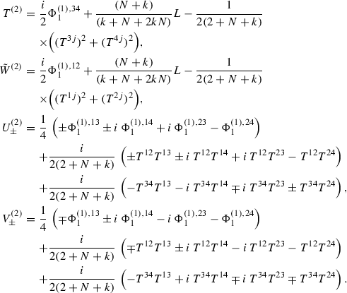
6.4 Eigenvalue equation of higher spin 2, 3, 4 currents
Let us obtain the eigenvalue equations for the higher spin 2 current (5.8) acting on the states \( |(f;0)>_{\pm }\). Only the \(Q^a(z)\) independent terms can contribute to the zero mode eigenvalue equations [16, 22]. The zero mode of the spin 1 current \(V^a(z)\) plays the role of the generator \(T_{a^{*}}\) of \(\mathrm{SU}(N+2)\) where \([T_a, T_b]= f_{ab}^{\,\,\,\,\,\,c} T_c\). See also footnote 6. We summarize the eigenvalue equations as follows:
For the second simplest representation, the eigenvalue equations can be obtained by calculating the OPE between the higher spin current and the spin \(\frac{1}{2}\) current \(Q^{\bar{A}*}\) in (6.3) and reading off the highest order pole [16, 22]. The terms containing the spin 1 current \(V^a(z)\) do not contribute to the highest order pole. We summarize the eigenvalue equations as follows:
Therefore, by using (6.24), (5.8) and (5.10), the eigenvalue equations of the zero mode of the higher spin 2 current (the more general expression) acting on the states \( |(f;0)>_{\pm }\) are given by
Similarly, the eigenvalue equations of the zero mode of the higher spin 2 current acting on the states \( |(0;f)>_{\pm }\), from (5.8), (5.10) and (6.25), are given by
The overall factors inside of the bracket have \(N \leftrightarrow k\) symmetry in (6.26) and (6.27).
By assuming that the two eigenvalues have the \(N \leftrightarrow k\) symmetryFootnote 19
where the large N ’t Hooft limit is taken, one can determine the two undetermined coefficients as follows:Footnote 20
The relations of the zero modes of the higher spin 3 currents (which are not described explicitly in this paper but we do have them for several N values explicitly) acting on the states \(|(f;0)>_{\pm }\) are, together with (6.26), given by
The first and last one in (6.33) satisfy eigenvalue equations. Furthermore, the zero modes of the higher spin 3 currents acting on the states \(|(0;f)>_{\pm }\), together with (6.27), satisfy
In this case, the first and the last one in (6.34) satisfy the eigenvalue equations.
The behaviors of (6.33) and (6.34) look similar to (6.8) and (6.9), respectively. The signs are the same.
Finally, the zero modes of the higher spin 4 current (which is not described explicitly in this paper but we do have this for several N values explicitly) acting on the states \(|(f;0)>_{\pm }\) and \(|(0;f)>_{\pm }\) are given by
There is \(N \leftrightarrow k\) symmetry. Note that the extra factors in the brackets in (6.35) behave as \(\frac{12}{5}(2+\lambda )\) (which is proportional to \((1+\lambda )\) plus one) and \(-\frac{12}{5}(3-\lambda )\) (which is proportional to \((2-\lambda )\) plus one) in the large N ’t Hooft limit, respectively. During this calculation, the contributions come from the coefficients of in k, N in the first factor of denominator, and kN in the second factor of denominator and the coefficients of \(k^2 N\), and \(k N^2\) in the numerator (they are given by 1, 1, 30, 12 and 18). This implies that the above large N behavior in (6.30) is reasonable because one observes \((2+\lambda )\) and \((3-\lambda )\) respectively. The above eigenvalues are very similar to the ones in the orthogonal Wolf space coset case in [42] under the large N ’t Hooft limit. For the different choice in (6.31), the signs are coincident with each other.
Then the three-point functions with these two scalars from (6.33), (6.34) and (6.35) can be written as
The overall behavior of (6.36) looks similar to the previous ones in (6.12) in the sense that the three-point functions of the higher spin 3 currents have simple form where the overall coefficients do not depend on N and k explicitly. Of course, the other three-point functions for the higher spin 3 currents vanish.
6.5 Eigenvalue equation of higher spin 2, 3, 4 currents in the extension of the large \(\mathcal{N}=4\) linear superconformal algebra
In order to obtain the three-point functions of the higher spin currents in the linear version, one should determine the lowest higher spin 2 current in terms of the currents of \(\mathcal{N}=4\) linear superconformal algebra and the corresponding higher spin currents only. Now one describes the previous higher spin 2 current (5.11) by substituting L(z) and \(T^{\mu \nu }(z)\) into the linear ones using the relations (4.1) (the higher spin currents \(\Phi _0^{(1)}(z)\) and \(\Phi _0^{(2)}(z)\) remain the same)
Let us emphasize that the field contents in \(\hat{\Phi }_0^{(2)}(z)\) in the nonlinear version is the same as the ones \({\hat{\varvec{\Phi }}_0^{(2)}}(z)\) in the linear version. At the level of \(V^a(z)\) and \(Q^a(z)\), they are exactly the same quantities. We have checked that starting from the most general spin 2 current in (6.37), we can construct the remaining 15 higher spin currents and the resulting 16 higher spin currents satisfy the \(\mathcal{N}=4\) primary conditions characterized by Appendix A.2 for generic \(\hat{a}_1\) and \(\hat{a}_2\). Then one has Eqs. (4.7) with hat notation.
One can evaluate the relevant equations for the zero mode of the higher spin 3 currents acting on the state (again the \(c_1\) term in (4.7) does not contribute the eigenvalue equations)
Furthermore, the other relevant equations lead to the following results:
In this case, the first and the last one in (6.39) satisfy the eigenvalue equations. They are the same as (6.33) and (6.34), respectively.
Finally, the zero modes of the ‘nonprimary’ higher spin 4 currents acting on the states \(|(f;0)>_{\pm }\) and \(|(0;f)>_{\pm }\) are given byFootnote 21
As in (6.17), all the N and k dependence in the combinations of the coefficients and the eigenvalues in (6.40) and (6.41) disappear.
On the other hand, in the primary basis, using (6.18) with hat, (6.42), (6.40) and (6.41), the following relations hold:
As described before, this reduces to (6.42) for \(k=N\). In this case, the results in (6.43) coincide with the ones in (6.35) in the large N ’t Hooft limit.Footnote 22 Again the large N ’t Hooft limit behavior of (6.43) looks similar to the ones in the orthogonal coset case in [42].
Let us summarize the three-point functions of the higher spin 2, 3, 4 currents from (6.38), (6.39), (6.42) and (6.43) as follows:
Therefore, the three-point functions in (6.45) have simple forms which are multiples of the eigenvalues of the higher spin 2 current in (6.26) and (6.27) even at finite N and k except of the last two. The other three-point functions for the higher spin 3 currents vanish. Compared to the nonlinear case (6.36), the only last two in (6.45) are different from each other at finite N and k.
7 Higher spin extension of \(\mathrm{SO}(\mathcal{N}=4)\) Knizhnik Bershadsky algebra in the Wolf space
As an application of the OPEs between the 16 currents described in previous sections, the extension of \(\mathrm{SO}(\mathcal{N}=4)\) Knizhnik Bershadsky algebra is analyzed.
7.1 \(\mathrm{SO}(\mathcal{N}=4)\) Knizhnik Bershadsky algebra from the large \(\mathcal{N}=4\) nonlinear superconformal algebra with the condition \(k=N\)
The Knizhnik Bershadsky algebra [36, 37] generated by the stress energy tensor \(T_{\mathrm{KB}}(z)\) of spin 2, the four spin \(\frac{3}{2}\) currents \(G^{\mu }_{\mathrm{KB}}(z)\) where the vector index \(\mu =1,2, \ldots , \mathcal{N}=4\), and the spin 1 currents \(J_{\mathrm{KB}}^a(z)\) where the adjoint index \(a=1,2, \ldots , \frac{1}{2}\mathcal{N}(\mathcal{N}-1)=6\) can be described as
The explicit \(\mathrm{SO}(\mathcal{N}=4)\) generators \(T_{\mu \nu }^a\) are given in Appendix C. The central charge is given by \(c=3k\) (or \(c=3N\)) where \(k =1, 2, \ldots \). The Wolf space central charge \(c_\mathrm{W}=\frac{3k^2}{(k+1)}\). Then it is straightforward to check that by identifying the following relations:
one sees that the above Knizhnik Bershadsky algebra (7.1) leads to the previous large \(\mathcal{N}=4\) nonlinear superconformal algebra. In Appendix D, we present the corresponding Appendix A in this case.
7.2 Higher spin extension of \(\mathrm{SO}(\mathcal{N}=4)\) Knizhnik Bershadsky algebra in the Wolf space
Then one obtains the higher spin extension of \(\mathrm{SO}(\mathcal{N}=4)\) Knizhnik Bershadsky algebra in the Wolf space and they are described in Appendix B together with (7.2) and \(k=N\). In Appendix E, the various coefficients in terms of k are given explicitly.
7.3 The \(\mathrm{SO}(\mathcal{N}=3)\) Knizhnik Bershadsky algebra and its extension
By taking the following choices from the currents in the linear version:
one obtains the \(\mathrm{SO}(\mathcal{N}=3)\) Knizhnik Bershadsky algebra [36, 37]. By adding the fermion \(\mathbf{\Gamma ^4}(z)\) to (7.3), one obtains the \(\mathcal{N}=3\) linear superconformal algebra [44,45,46]. The central term coming from the fourth order term in the OPE between the \(\hat{T}(z)\) and \(\hat{T}(w)\) is given by \(\frac{1}{4}(5+3k+3N)\).
Then one can see that the previous results in [6] provide the higher spin extension of the \(\mathrm{SO}(\mathcal{N}=3)\) Knizhnik Bershadsky algebra.
8 Conclusions and outlook
First of all, we have obtained the OPEs in Appendix A.2 which were necessary to calculate the higher spin \(\frac{5}{2}, 3, \frac{7}{2}, 4\) currents in the next 16 higher spin currents. For the bosonic higher spin 3, 4 currents, their expressions in terms of WZW currents for several N can be read off from the defining relations in Appendix A.2.
Secondly, we also have determined the OPEs between the lowest 16 higher spin currents in Appendix B. One of the motivations to obtain these is to describe the marginal deformation which breaks the higher spin symmetry and determine the mass for the higher spin currents in the large (N, k) ’t Hooft limit. The coset model we consider here has \(\mathcal{N}=4\) supersymmetry and there should be a marginal deformation [47]. It would be interesting to determine the mass for the higher spin currents with the help of the explicit symmetry algebra found in this paper. According to the observation of [48,49,50], the \(\mathrm{SO}(2)_R\) doublet rather than \(\mathrm{SO}(2)_R\) singlet can have nonzero mass contribution. See also the relevant work in [51]. It is well known that the divergence of higher spin-s currents contains some operator which breaks the higher spin symmetry [52]. Although the explicit form for the perturbing marginal operator which transforms as a nontrivial primary state from the denominator of the coset is not determined yet, one can analyze further by assuming that there exist the eigenvalue equations for the zeromodes of the spins \(s=1,2,3\) acting on the state associated with the perturbing operator [53]. The anormalous dimension of the higher spin current at the leading order corresponds to the norm of the above divergence of the corresponding higher spin current [48]. Then from our result, one obtains the commutation relations \([\Phi _{1,m}^{(1),\mu \nu },\Phi _{1,n}^{(1),\rho \sigma }]\) and \([\Phi _{1,m}^{(2)},\Phi _{1,n}^{(2)}]\) as well as the standard commutators \([L_m,L_n]\), \([L_m, \Phi _{1,n}^{(1),\mu \nu }]\) and \([L_m, \Phi _{1,n}^{(2)}]\). Then one can write down the various modes between the states from the higher spin symmetry breaking terms. By moving the positive modes to the right in the corresponding terms, and using the commutators and the eigenvalue equations, we will obtain the coefficient of the norm of perturbing marginal operator which depends on the eigenvalues. It would be interesting to find the perturbing marginal operator explicitly and describe the mass terms with the explicit eigenvalues further.
Thirdly, the lowest higher spin 2 current (5.8) or (5.11) in the next 16 higher spin currents was found explicitly in terms of WZW currents. The sixth and ninth terms having the quadratic \(d^{0}_{\bar{a}\bar{b}}\) tensors (3.5) are new compared to the orthogonal case [42]. They come from the quadratic higher spin 1 currents in (3.4). It would be interesting to obtain the remaining higher spin \(\frac{5}{2}, 3, \frac{7}{2}, 4\) currents in (1.1) in terms of spin 1 and spin \(\frac{1}{2}\) currents for generic N and k. This can be done manually by using Appendix A.2 along the line of [15] or one can read off the relative coefficients appearing in the possible terms from the explicit results for several N cases. For the latter, it is nontrivial to obtain the possible terms completely.
Fourthly, the three-point functions in (6.36) and (6.45) were obtained. For the \(\mathrm{SO}(4)\) adjoint higher spin 3 currents, the three-point functions are the same in nonlinear and linear versions. For the spin 4 current, the \(N \leftrightarrow k\) symmetry appears in the nonlinear version as in the stress energy tensor of spin 2 in (6.4). As described before, these three-point functions look similar to the ones in [42] in the sense that the \(\lambda \) dependence appearing in the three-point functions coincides with each other.
It is straightforward to apply the work of [6] and the presentation of this paper to the orthogonal case [54] in the context of [55,56,57,58,59]. The lowest 16 higher spin currents contains the higher spin 2 current as its lowest component. The complete OPEs between the lowest higher spin 2 currents can be constructed and it turns out that there are next 16 higher spin currents containing the higher spin 3 current as its lowest component in the right hand sides of the OPEs. Moreover, there are three different next 16 higher spin currents. They transform as \(\mathrm{SO}(3)\) triplet inside of \(\mathrm{SO}(4)\) rather than a singlet. Furthermore, the third 16 higher spin currents containing the higher spin 4 current as its lowest component appear in the right hand sides of the OPEs. It would be interesting to describe this orthogonal case in detail.
Recently, the other type of large \(\mathcal{N}=4\) holography is studied in [60]. It is an open problem to study this holography in the context of \(\mathcal{N}=4\) coset model.
One can also consider (i) the fermionic higher spin current-scalar-spinor three-point functions as well as the three-point functions, given by (ii) the bosonic higher spin current-scalar-spinor, (iii) the bosonic higher spin current-spinor-spinor, (iv) the fermionic higher spin current-scalar-scalar, and (v) the fermionic higher spin current-spinor-spinor. The states corresponding to the spinors can be obtained by acting the spin \(\frac{3}{2}\) currents \(G^{\mu }\) on the states \(|(f;0)>\) or \(|(0;f)>\) [61, 62]. For example, one should calculate the four-point functions \(<{\overline{\mathcal{O}}}_{\pm } \mathcal{O}_{\pm } \, G^{\mu } \, \Phi ^{(1),\nu }_{\frac{1}{2}}>\) for case (i) when we take the simplest fermionic higher spin-\(\frac{3}{2}\) currents. The corresponding OPE \(G^{\mu }(z_1) \, \Phi ^{(1),\nu }_{\frac{1}{2}}(z_2)\) in this four-point function is given in Appendix A.2. The normal ordered product \((G^{\mu } \, \Phi ^{(1),\nu }_{\frac{1}{2}})(z_2)\) appears in the zeroth order [39] and the positive power of \((z_1-z_2)\) has the form of \( \sum _{n=1}^{\infty } \frac{1}{n!} \, (z_1-z_2)^n \, (\partial ^n G^{\mu } \, \Phi ^{(1),\nu }_{\frac{1}{2}})(z_2)\). By analyzing the contributions of zero modes in the field dependent parts (appearing in the singular and regular terms) in the states, the above four-point functions can be determined together with \(z_1\) and \(z_2\) dependences as in Sect. 6.
For case (ii), one can use the OPE \(G^{\mu }(z_1) \, \Phi ^{(1)}_{0}(z_2)\), for example, when one considers the simplest bosonic higher spin current. The previous analysis for case (i) can be done.
For case (iii), one should analyze the five-point functions \(<{\overline{\mathcal{O}}}_{\pm } \mathcal{O}_{\pm } \, G^{\mu } \, \Phi ^{(1)}_{0} \, G^{\nu }>\) where the \(\mu \) and \(\nu \) indices are complex conjugated to each other. We take the simplest higher spin-1 current here. The operator \( G^{\mu }(z_1) \, \Phi ^{(1)}_{0}(z_2) \, G^{\nu }(z_3) \) consists of four pieces [63]. That is,
where the notation \(:A(z_1) \, B(z_2):\) means all the regular (or nonsingular) terms of the OPE \(A(z_1) \, B(z_2)\) [63]. One has all the three OPEs, \( G^{\mu }(z_1) \, \Phi ^{(1)}_{0}(z_2)\), \(\Phi ^{(1)}_{0}(z_2) \, G^{\nu }(z_3)\) and \(G^{\mu }(z_1) \, G^{\nu }(z_3)\) from Appendices A.1 and A.2. In the first term of (8.1), one should take the regular terms in the OPE \( G^{\mu }(z_1)\) and the \(z_3\) dependent fields in the OPE of \( \Phi ^{(1)}_{0}(z_2) \, G^{\nu }(z_3)\). Similarly, for the second term, one should take the regular terms in the OPE between the \(z_2\) dependent fields appearing in the OPE \(G^{\mu }(z_1) \, \Phi ^{(1)}_{0}(z_2)\) and \(G^{\nu }(z_3)\). One can also extract the nontrivial \(z_3\) dependent terms in the remaining third and fourth terms of (8.1). After that, one should calculate the OPEs with the first factors. By analyzing the contributions of zero modes in the field dependent parts appearing in the singular and regular terms in the states, one can calculate the five-point functions including the \(z_1, z_2\) and \(z_3\) dependences.
For case (iv), one should examine the zero mode contributions in the fermionic higher spin currents as in Sect. 6.
For case (v), one should analyze the five-point functions \(<{\overline{\mathcal{O}}}_{\pm } \mathcal{O}_{\pm } \, G^{\mu } \, \Phi ^{(1), \nu }_{\frac{1}{2}} \, G^{\rho }>\) with simplest higher spin-\(\frac{3}{2}\) currents. This can be done as in previous case (iii).
What happens for the three-point and four-point functions between the higher spin currents with vacuum \(|0>\)? For example, one can easily see that the two-point function in the higher spin-1 current is
from the result of Appendix B.1. Note that \(z_{12} \equiv (z_1-z_2)\). One sees that the three-point function in the higher spin-1 current \( <0| \Phi _0^{(1)}(z_1) \, \Phi _0^{(1)}(z_2) \, \Phi _0^{(1)}(z_3)|0> \) vanishes by analyzing the four contributions in the vacuum as in (8.1). For the four-point function, one can use the equation (2.64) of [63] where the difference between the OPE and the vacuum expectation value of the OPE is introduced in (2.59) of [63]. Then it is easy to see that this quantity corresponding to the above OPE \(\Phi _0^{(1)}(z_1) \, \Phi _0^{(1)}(z_2)\) vanishes. Then the four-point function can be reduced to three contributions from the product of two-point functions. It turns out that
For the four-point functions having other higher spin currents, the similar analysis (after further OPEs can be found) can be done.
Recall that the state \(| (0;f)>\) contains the vacuum \(|0>\) in (6.3). The four-point function \(<{\overline{\mathcal{O}}}_{-} \mathcal{O}_{-} \, \Phi _0^{(1)} \, \Phi ^{(1),\mu \nu }_{1}>\) can be related to \(<0| Q^{a}(z_1) \, \Phi _0^{(1)}(z_2) \, \Phi ^{(1),\mu \nu }_{1}(z_3) \, Q^{\bar{b}}(z_4) |0>\). Because the OPEs between the higher spin currents and spin-\(\frac{1}{2}\) currents are known explicitly, one can calculate the four-point functions.
Notes
The terminology ‘large’ here (we do not take any limit) is nothing to do with the one in the large N ’t Hooft like limit later.
The higher spin currents (with boldface notation) in the ‘linear’ version are defined as the ones in the extension of the large \(\mathcal{N}=4\) ‘linear’ superconformal algebra while the higher spin currents in the ‘nonlinear’ version are defined as the ones in the extension of the large \(\mathcal{N}=4\) ‘nonlinear’ superconformal algebra. The OPEs between the higher spin currents in the linear (and nonlinear) version are nonlinear.
One can also try to obtain these OPEs from the results of [14] by introducing the arbitrary coefficients in the right hand sides of the OPEs and using the Jacobi identities.
There is also another consistency check which can be described as the matching of BPS spectrum in both sides. Recently, in [17], by analyzing the BPS spectrum of string theory and supergravity theory on \(AdS_3 \times \mathbf{S}^3 \times \mathbf{S}^3 \times \mathbf{S}^1\), it has been found that the BPS spectra of both descriptions agree. It would be interesting to obtain the BPS spectrum in the \(\mathcal{N}=4\) coset theories and see whether this matches with the findings in [17]. See also [18].
In the linear version there are additional terms also: the quadratic in the spin 1 current, the product of spin 1 current and the two spin \(\frac{1}{2}\) currents with \(\mathrm{SO}(4)\) Kronecker deltas, the product of spin 1 current and the two spin \(\frac{1}{2}\) currents with \(\mathrm{SO}(4)\) epsilon tensor, the quartic terms in the spin \(\frac{1}{2}\) currents with \(\mathrm{SO}(4)\) epsilon tensor and the quadratic terms in the spin \(\frac{1}{2}\) currents with a derivative. See also Eq. (6.37). Note that the higher spin 2 current living in the next 16 higher spin currents in the nonlinear version is the same as the one in the linear version. They have the same WZW currents.
Let us emphasize that there is a summation over index c in the spin 1 current \(A^{+i}(z)\) and this c runs over \(c=1, 2, \ldots , \frac{1}{2}[(N+2)^2-1], 1^{*}, 2^{*}, \ldots , \frac{1}{2}[(N+2)^2-1]^{*}\) along the line of (2.2). This behavior also occurs in the spin 2 stress energy tensor T(z). The remaining summations run over the coset indices where \(\bar{a}, \bar{b}, \ldots = 1, 2, \ldots , 2N, 1^{*}, 2^{*}, \ldots , 2N^{*}\) with (2.3). Note that one obtains \( [V^a_m, V^b_n] = k m g^{ab} \delta _{m+n,0} - f^{ab}_{\,\,\,\,\,\,c} V^c_{m+n} \) from (2.5). For the indices \(m=0=n\), this leads to \([V^a_0, V^b_0] = - f^{ab}_{\,\,\,\,\,\,c} V^c_0\), which is related to the commutation relations of the underlying finite dimensional Lie algebra \(\mathrm{SU}(N+2)\).
The explicit relations between the 11 currents in two bases are given by
$$\begin{aligned}T(z) \rightarrow L(z), \quad G^0(z) \rightarrow G^2(z), \quad G^1(z) \rightarrow G^3(z), \quad \nonumber \\ G^2(z) \rightarrow -G^4(z), \quad G^3(z) \rightarrow G^1(z), \nonumber \\ A^{\pm 1}(z)\rightarrow {} \frac{i}{2} \left( T^{14} \mp T^{23}\right) (z) = \frac{i}{2} \, \alpha _{\mu \nu }^{\pm 1} \, T^{\mu \nu }(z), \quad \nonumber \\ A^{\pm 2}(z)\rightarrow {} \frac{i}{2} \left( T^{13} \pm T^{24}\right) (z) =\frac{i}{2} \, \alpha _{\mu \nu }^{\pm 2} \, T^{\mu \nu }(z), \nonumber \\ A^{\pm 3}(z)\rightarrow {} \pm \frac{i}{2} \left( T^{12} \mp T^{34}\right) (z)= \frac{i}{2} \, \alpha _{\mu \nu }^{\pm 3} \, T^{\mu \nu }(z), \end{aligned}$$(2.9)where the previous quantity in (2.8) with the renaming of the indices is changed into
$$\begin{aligned} \alpha ^{\pm 1}_{\mu \nu }= & {} \left( \begin{array}{llll} 0 &{}\quad \!\! 0 &{}\quad \!\! 0 &{}\quad \!\! \frac{1}{2} \\ 0 &{}\quad \!\! 0 &{}\quad \!\! \mp \frac{1}{2} &{}\quad \!\! 0 \\ 0 &{}\quad \!\! \pm \frac{1}{2} &{}\quad \!\! 0 &{}\quad \!\! 0 \\ -\frac{1}{2} &{}\quad \!\! 0 &{}\quad \!\! 0 &{}\quad \!\! 0 \\ \end{array} \right) ,\quad \alpha ^{\pm 2}_{\mu \nu } = \left( \begin{array}{cccc} 0 &{}\quad \!\! 0 &{}\quad \!\! \frac{1}{2} &{}\quad \!\! 0 \\ 0 &{}\quad \!\! 0 &{}\quad \!\! 0 &{}\quad \!\! \pm \frac{1}{2} \\ - \frac{1}{2} &{}\quad \!\! 0 &{}\quad \!\! 0 &{}\quad \!\! 0 \\ 0 &{}\quad \!\! \mp \frac{1}{2} &{}\quad \!\! 0 &{}\quad \!\! 0 \\ \end{array} \right) ,\quad \alpha ^{\pm 3}_{\mu \nu } = \left( \begin{array}{cccc} 0 &{}\quad \!\! \pm \frac{1}{2} &{}\quad \!\! 0 &{}\quad \!\! 0 \\ \mp \frac{1}{2} &{}\quad \!\! 0 &{}\quad \!\! 0 &{}\quad \!\! 0 \\ 0 &{}\quad \!\! 0 &{}\quad \!\! 0 &{}\quad \!\! - \frac{1}{2} \\ 0 &{}\quad \!\! 0 &{}\quad \!\! \frac{1}{2} &{}\quad \!\! 0 \\ \end{array} \right) . \end{aligned}$$(2.10)One can consider this 16 higher spin currents (3.1) in \(\mathrm{SU}(2) \times SU(2)\) basis [12] and their precise relations are given as follows:
$$\begin{aligned}&V_0^{(s)}(z) = -i \, \Phi _0^{(s)}(z), \quad V_{\frac{1}{2}}^{(s),1}(z) = i \, \Phi _{\frac{1}{2}}^{(s),1}(z), \quad V_{\frac{1}{2}}^{(s),2}(z) = -i \, \Phi _{\frac{1}{2}}^{(s),2}(z),\quad V_{\frac{1}{2}}^{(s),3}(z) = -i \, \Phi _{\frac{1}{2}}^{(s),3}(z),\quad V_{\frac{1}{2}}^{(s),4}(z) = -i \, \Phi _{\frac{1}{2}}^{(s),4}(z), \quad \nonumber \\&V_{1}^{(s), \pm i}=\mp i \alpha ^{\pm i}_{\mu \nu }\,\Phi _{1}^{(s),\mu \nu },\quad V_{\frac{3}{2}}^{(s), 1}(z) = -2 i \, \Phi _{\frac{3}{2}}^{(s), 1}(z), \quad V_{\frac{3}{2}}^{(s), 2}(z) = 2 i \, \Phi _{\frac{3}{2}}^{(s), 2} (z), V_{\frac{3}{2}}^{(s), 3}(z) = 2 i \, \Phi _{\frac{3}{2}}^{(s), 3}(z), \quad V_{\frac{3}{2}}^{(s), 4}(z) = 2 i \, \Phi _{\frac{3}{2}}^{(s), 4} (z), \nonumber \\&V_{2}^{(s)}(z) = 2i\,\Bigg [\,\Phi _{2}^{(s)} \,{-}\, \frac{24 i (k \,{-}\, N) s (1 \,{+}\, s)}{3 k \,{+}\, 3 N \,{+}\, 6 k N \,{-}\, 20 s \,{-}\, 4 k s \,{-}\, 4 N s \,{+}\, 12 k N s \,{+}\, 32 s^2 \,{+}\, 16 k s^2 \,{+}\, 16 N s^2}\,L\Phi _{0}^{(s)} \nonumber \\&\,{+}\, \frac{36 i (k \,{-}\, N) s (1 \,{+}\, s)}{(1 \,{+}\, 2 s) (3 k \,{+}\, 3 N \,{+}\, 6 k N \,{-}\, 20 s \,{-}\, 4 k s \,{-}\, 4 N s \,{+}\, 12 k N s \,{+}\, 32 s^2 \,{+}\, 16 k s^2 \,{+}\, 16 N s^2)}\partial ^2 \Phi _{0}^{(s)}\,\Bigg ](z), \end{aligned}$$(3.2)where the \(\alpha _{\mu \nu }^{\pm i}\) tensor can be obtained from the ones in [12] by changing the sign of index 1 appearing in the row or column of \(\alpha _{\mu \nu }^{\pm i}\) in [12],
$$\begin{aligned} \alpha ^{\pm 1}_{\mu \nu }= & {} \left( \begin{array}{cccc} 0 &{} 0 &{} 0 &{} \mp \frac{1}{2} \\ 0 &{} 0 &{} \frac{1}{2} &{} 0 \\ 0 &{} - \frac{1}{2} &{} 0 &{} 0 \\ \pm \frac{1}{2} &{} 0 &{} 0 &{} 0 \\ \end{array} \right) ,\quad \alpha ^{\pm 2}_{\mu \nu } = \left( \begin{array}{cccc} 0 &{} 0 &{} \frac{1}{2} &{} 0 \\ 0 &{} 0 &{} 0 &{} \pm \frac{1}{2} \\ - \frac{1}{2} &{} 0 &{} 0 &{} 0 \\ 0 &{} \mp \frac{1}{2} &{} 0 &{} 0 \\ \end{array} \right) , \alpha ^{\pm 3}_{\mu \nu } = \left( \begin{array}{cccc} 0 &{} - \frac{1}{2} &{} 0 &{} 0 \\ \frac{1}{2} &{} 0 &{} 0 &{} 0 \\ 0 &{} 0 &{} 0 &{} \pm \frac{1}{2} \\ 0 &{} 0 &{} \mp \frac{1}{2} &{} 0 \\ \end{array} \right) . \end{aligned}$$(3.3)The locations for the nonzero elements in (3.3) are the same as the previous ones (2.10). There are \((\mathbf{1},\mathbf{1})\) for \(V_0^{(s)}(z)\), \((\mathbf{2},\mathbf{2})\) for \(V_{\frac{1}{2}}^{(s),\mu }(z)\), \((\mathbf{3},\mathbf{1}) \oplus (\mathbf{1},\mathbf{3})\) for \(V_1^{(s), \pm i}(z)\), \((\mathbf{2},\mathbf{2})\) for \(V_{\frac{3}{2}}^{(s),\mu }(z)\), and \((\mathbf{1},\mathbf{1})\) for \(V_2^{(s)}(z)\) under the \(\mathrm{SU}(2) \times \mathrm{SU}(2)\).
One should change the index structures as follows: \(\mathbf{\Gamma ^0} \rightarrow -i \mathbf{\Gamma ^2}\), \(\mathbf{\Gamma ^1} \rightarrow -i \mathbf{\Gamma ^3}\), \(\mathbf{\Gamma ^2} \rightarrow i \mathbf{\Gamma ^4}\) and \(\mathbf{\Gamma ^3} \rightarrow -i \mathbf{\Gamma ^1}\) in order to use (4.1) from (4.2). We introduce the coset \(\frac{G}{H}=\frac{\mathrm{SU}(N+2)}{\mathrm{SU}(N)}\) notation \(\tilde{a}=(\bar{a}, \hat{a})\) where the \(\bar{a}\) index runs over 4N values as before and the index \(\hat{a}\) associates with the \(2 \times 2\) matrix corresponding to \(\mathrm{SU}(2)\times U(1)\) and runs over 4 values. Let us represent the \(4 \times 4\) matrices \(h^{i}_{\hat{a} \hat{b}}\) appearing in (4.2) as follows [22]:
 (4.3)
(4.3)where the quantity A in (4.3) which depends on N is given by
 (4.4)
(4.4)The \(\hat{a}\) indices are given by \((2N+1)\), \(\frac{1}{2}[(N+2)^2-1]\), \((2N+1)^*\) and \(\frac{1}{2}[(N+2)^2-1]^{*}\) of (2.4). The N dependence in (4.4) can be fixed by the several N cases.
The relations between the spin 1 currents in two different bases are given by
 (4.10)
Or one can express these in (4.10) as \(\mathbf{T^{\mu \nu }}(z) = -2i \, \alpha _{\mu \nu }^{+i} \, \mathbf{A^{+i}}-2i \, \alpha _{\mu \nu }^{-i} \, \mathbf{A^{-i}}\) where \(\alpha _{\mu \nu }^{\pm i}\) are given in (2.10).
In the description of \(\mathcal{N}=2\) superspace multiplets [22], one has explicit relations between the higher spin 2 currents as follows:
 (6.7)
(6.7)It is straightforward to obtain the eigenvalue equations [22] of the left hand sides of (6.7) by using the expressions of the right hand sides of (6.7), the Eqs. (6.8) and (6.9) and other relevant relations.
One has the following explicit relation between the higher spin 3 currents:
$$\begin{aligned} W^{(3)}(z)= & {} -\frac{1}{2}\,\Phi _2^{(1)}(z)+\frac{1}{(2+N+k)} \Bigg [\,\frac{i}{2}\,\partial \Phi _{1}^{(1),12}-i\,T^{12}\Phi _{1}^{(1),12}\nonumber \\&+2i\,T^{34}\Phi _{1}^{(1),34} + \frac{i}{2}\left( \,T^{1j}\Phi _{1}^{(1),1j}+\,T^{2j}\Phi _{1}^{(1),2j}\right) \nonumber \\&+\frac{1}{2}\left( \,T^{1j}\Phi _{1}^{(1),2j}-\,T^{2j}\Phi _{1}^{(1),1j}\right) \nonumber \\&-\left( T^{34}\partial \Phi _{0}^{(1)}-\partial T^{34}\Phi _{0}^{(1)}\right) \nonumber \\&-2i\, G^{1}G^{2}+\frac{16(1+N+k)}{(4+5k+5N+6kN)}\,T^{12}L\nonumber \\&-\frac{4(k-N)}{(4+5k+5N+6kN)}\,T^{34}L \,\Bigg ](z)+ \frac{1}{(2+N+k)^{2}}\, \nonumber \\&\Bigg [\, 2\,(T^{12})^{3}-\Big (T^{12}(T^{1j})^{2}+ T^{12}(T^{2j})^{2}\Big )-4\,T^{12}(T^{34})^{2} \nonumber \\&+2\,\varepsilon ^{12ij}\,T^{1i}T^{2j}T^{34}+ (N-k)\,\left( T^{12}\partial T^{34}-\partial T^{12}T^{34}\right) \nonumber \\&+\frac{i(N-k)}{2}\,\left( T^{1j}\partial \tilde{T}^{2j}-T^{2j}\partial \tilde{T}^{1j}\right) \nonumber \\&-\frac{i(-8+N+k)}{2}\,T^{1j}\partial T^{2j}+\frac{i(N+k)}{2}\,\partial T^{1j}T^{2j}\nonumber \\&+\frac{(-12+5N+5k)}{6}\,\partial ^{2}T^{12}+\frac{4(-N+k)}{3}\,\partial ^{2}T^{34} \,\Bigg ](z).\nonumber \\ \end{aligned}$$(6.10)Moreover, one can check the eigenvalue equations of the higher spin 3 current \(W^{(3)}(z)\) [22] by using the relation (6.10) and other relevant relations including (6.11).
One can calculate the eigenvalue equations for the extra terms in (4.7).:
 (6.15)
Similarly, one has the following eigenvalue equations:
 (6.16)
The precise relations between the higher spin currents in two different bases are given by
 (6.21)
One can obtain the corresponding eigenvalue equations for the higher spin currents appearing in the left hand sides of (6.21) by using these relations.
One can calculate the eigenvalue equations for the extra terms in (4.7)
 (6.40)
Similarly, one has the following eigenvalue equations:
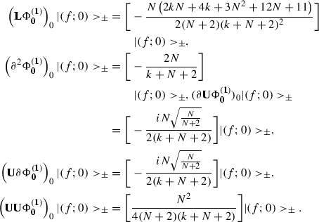
$$\begin{aligned}&\left( {\mathbf{L} \hat{\varvec{\Phi }}_{\mathbf{0}}^{(\mathbf{2})}}\right) _0 |(0;f)>_{\pm }\nonumber \\&\quad = \Bigg [ \frac{(5 k N+4 N^2+10 N+1)}{2 N (k+N+2)} \Bigg ] ( \hat{\phi }_0^{(2)})_{(0;f)} |(0;f)>_{\pm }, \nonumber \\&\left( \partial ^{2} {\hat{\varvec{\Phi }}_{\mathbf{0}}^{(\mathbf{2})}}\right) _0 |(0;f)>_{\pm } = \Bigg [ 6 \Bigg ] ( \hat{\phi }_0^{(2)})_{(0;f)} |(0;f)>_{\pm }, \nonumber \\&\left( \partial {\mathbf{U} \hat{\varvec{\Phi }}_{\mathbf{0}}^{(\mathbf{2})}}\right) _0 |(0;f)>_{\pm } = \Bigg [ \frac{1}{2} i \sqrt{\frac{(N+2)}{N}} \Bigg ] ( \hat{\phi }_0^{(2)})_{(0;f)} |(0;f)>_{\pm }, \nonumber \\&\left( \mathbf{U } \partial {\hat{\varvec{\Phi }}_{\mathbf{0}}^{(\mathbf{2})}} \right) _0 |(0;f)>_{\pm } = \Bigg [ i \sqrt{\frac{(N+2)}{N}} \Bigg ] ( \hat{\phi }_0^{(2)})_{(0;f)} |(0;f)>_{\pm }, \nonumber \\&\left( {\mathbf{U U} \hat{\varvec{\Phi }}_{\mathbf{0}}^{(\mathbf{2})}}\right) _0 |(0;f)>_{\pm } = \Bigg [ -\frac{(N+2)}{4 N} \Bigg ] ( \hat{\phi }_0^{(2)})_{(0;f)} |(0;f)>_{\pm },\nonumber \\ \end{aligned}$$(6.41)It is easy to check that the extra terms vanish under the large N ’t Hooft limit. One obtains the differences of each eigenvalue as follows:
 (6.44)
Then in the large N ’t Hooft limit, these (6.44) vanish.


References
A. Sevrin, W. Troost, A. Van Proeyen, Superconformal algebras in two-dimensions with N = 4. Phys. Lett. B 208, 447 (1988). doi:10.1016/0370-2693(88)90645-4
A. Sevrin, W. Troost, A. Van Proeyen, P. Spindel, Extended supersymmetric sigma models on group manifolds. 2. Current algebras. Nucl. Phys. B 311, 465 (1988). doi:10.1016/0550-3213(88)90070-3
K. Schoutens, O(n) extended superconformal field theory in superspace. Nucl. Phys. B 295, 634 (1988). doi:10.1016/0550-3213(88)90539-1
A. Sevrin, G. Theodoridis, N = 4 superconformal coset theories. Nucl. Phys. B 332, 380 (1990). doi:10.1016/0550-3213(90)90100-R
N. Saulina, Geometric interpretation of the large N = 4 index. Nucl. Phys. B 706, 491 (2005). doi:10.1016/j.nuclphysb.2004.11.049. arXiv:hep-th/0409175
C. Ahn, M.H. Kim, The operator product expansion between the 16 lowest higher spin currents in the \({\cal{N}}=4\) superspace. Eur. Phys. J. C 76(7), 389 (2016). doi:10.1140/epjc/s10052-016-4234-2. arXiv:1509.01908 [hep-th]
C. Ahn, Higher spin currents in Wolf space: III. Class. Quantum Gravity 32(18), 185001 (2015). doi:10.1088/0264-9381/32/18/185001. arXiv:1504.00070 [hep-th]
P. Goddard, A. Schwimmer, Factoring out free fermions and superconformal algebras. Phys. Lett. B 214, 209 (1988). doi:10.1016/0370-2693(88)91470-0
A. Van Proeyen, Realizations of \(N=4\) superconformal algebras on wolf spaces. Class. Quantum Gravity 6, 1501 (1989). doi:10.1088/0264-9381/6/10/018
M. Gunaydin, J.L. Petersen, A. Taormina, A. Van Proeyen, On the unitary representations of a class of \(N=4\) superconformal algebras. Nucl. Phys. B 322, 402 (1989). doi:10.1016/0550-3213(89)90421-5
S.J. Gates Jr., S.V. Ketov, No N = 4 strings on wolf spaces. Phys. Rev. D 52, 2278 (1995). doi:10.1103/PhysRevD.52.2278. arXiv:hep-th/9501140
M. Beccaria, C. Candu, M.R. Gaberdiel, The large N = 4 superconformal \(W_{\infty }\) algebra. JHEP 1406, 117 (2014). doi:10.1007/JHEP06(2014)117. arXiv:1404.1694 [hep-th]
C. Ahn, Higher spin currents in wolf space. Part I. JHEP 1403, 091 (2014). doi:10.1007/JHEP03(2014)091. arXiv:1311.6205 [hep-th]
C. Ahn, Higher spin currents in wolf space: part II. Class. Quantum Gravity 32(1), 015023 (2015). doi:10.1088/0264-9381/32/1/015023. arXiv:1408.0655 [hep-th]
C. Ahn, H. Kim, Higher spin currents in wolf space for generic N. JHEP 1412, 109 (2014). doi:10.1007/JHEP12(2014)109. arXiv:1411.0356 [hep-th]
M.R. Gaberdiel, R. Gopakumar, Large N = 4 holography. JHEP 1309, 036 (2013). doi:10.1007/JHEP09(2013)036. arXiv:1305.4181 [hep-th]
L. Eberhardt, M.R. Gaberdiel, R. Gopakumar, W. Li, BPS spectrum on AdS\(_3\times \)S\(^3 \times \)S\(^3 \times \)S\(^1\). arXiv:1701.03552 [hep-th]
Gaberdiel’s talk at the conference, The First Mandalstam Theoretical Physics School and Workshop: Recent Advances in AdS/CFT, January 11–17, 2017, Durban, South Africa (2017)
M.R. Gaberdiel, R. Gopakumar, Higher spins & strings. JHEP 1411, 044 (2014). doi:10.1007/JHEP11(2014)044. arXiv:1406.6103 [hep-th]
M.R. Gaberdiel, R. Gopakumar, Stringy symmetries and the higher spin square. J. Phys. A 48(18), 185402 (2015). doi:10.1088/1751-8113/48/18/185402. arXiv:1501.07236 [hep-th]
M.R. Gaberdiel, R. Gopakumar, String theory as a higher spin theory. JHEP 1609, 085 (2016). doi:10.1007/JHEP09(2016)085. arXiv:1512.07237 [hep-th]
C. Ahn, H. Kim, Three point functions in the large \( \cal{N}=4 \) holography. JHEP 1510, 111 (2015). doi:10.1007/JHEP10(2015)111. arXiv:1506.00357 [hep-th]
M.R. Gaberdiel, T. Hartman, Symmetries of holographic minimal models. JHEP 1105, 031 (2011). doi:10.1007/JHEP05(2011)031. arXiv:1101.2910 [hep-th]
M.R. Gaberdiel, R. Gopakumar, T. Hartman, S. Raju, Partition functions of holographic minimal models. JHEP 1108, 077 (2011). doi:10.1007/JHEP08(2011)077. arXiv:1106.1897 [hep-th]
C. Ahn, The coset spin-4 casimir operator and its three-point functions with scalars. JHEP 1202, 027 (2012). doi:10.1007/JHEP02(2012)027. arXiv:1111.0091 [hep-th]
C. Ahn, The primary spin-4 casimir operators in the holographic SO(N) coset minimal models. JHEP 1205, 040 (2012). doi:10.1007/JHEP05(2012)040. arXiv:1202.0074 [hep-th]
C. Ahn, The higher spin currents in the N = 1 stringy coset minimal model. JHEP 1304, 033 (2013). doi:10.1007/JHEP04(2013)033. arXiv:1211.2589 [hep-th]
C. Ahn, Higher spin currents with arbitrary N in the \({\cal{N}} = 1\) stringy coset minimal model. JHEP 1307, 141 (2013). doi:10.1007/JHEP07(2013)141. arXiv:1305.5892 [hep-th]
C. Ahn, H. Kim, Spin-5 Casimir operator and its three-point functions with two scalars. JHEP 1401, 012 (2014). Erratum: [JHEP 1401, 174 (2014)]. doi:10.1007/JHEP01(2014)012, doi:10.1007/JHEP01(2014)174. arXiv:1308.1726 [hep-th]
C. Ahn, Higher spin currents in the orthogonal coset theory. arXiv:1701.02410 [hep-th]
M.R. Gaberdiel, R. Gopakumar, An \(AdS_3\) dual for minimal model CFTs. Phys. Rev. D 83, 066007 (2011). doi:10.1103/PhysRevD.83.066007. arXiv:1011.2986 [hep-th]
M.R. Gaberdiel, R. Gopakumar, Triality in minimal model holography. JHEP 1207, 127 (2012). doi:10.1007/JHEP07(2012)127. arXiv:1205.2472 [hep-th]
M.R. Gaberdiel, R. Gopakumar, Minimal model holography. J. Phys. A 46, 214002 (2013). doi:10.1088/1751-8113/46/21/214002. arXiv:1207.6697 [hep-th]
K. Thielemans, A mathematica package for computing operator product expansions. Int. J. Mod. Phys. C 2, 787 (1991). doi:10.1142/S0129183191001001
Wolfram Research, Inc., Mathematica, Version 11.0, Champaign (2016)
V.G. Knizhnik, Superconformal algebras in two-dimensions. Theor. Math. Phys. 66, 68 (1986). [Teor. Mat. Fiz. 66, 102 (1986)]. doi:10.1007/BF01028940
M.A. Bershadsky, Superconformal algebras in two-dimensions with arbitrary \(N\). Phys. Lett. B 174, 285 (1986). doi:10.1016/0370-2693(86)91100-7
V.G. Kac, I.T. Todorov, Superconformal current algebras and their unitary representations. Commun. Math. Phys. 102, 337 (1985). doi:10.1007/BF01229384
F.A. Bais, P. Bouwknegt, M. Surridge, K. Schoutens, Extensions of the Virasoro algebra constructed from Kac-Moody algebras using higher order Casimir invariants. Nucl. Phys. B 304, 348 (1988). doi:10.1016/0550-3213(88)90631-1
F.A. Bais, P. Bouwknegt, M. Surridge, K. Schoutens, Coset construction for extended Virasoro algebras. Nucl. Phys. B 304, 371 (1988). doi:10.1016/0550-3213(88)90632-3
J. Fuchs, More on the super WZW theory. Nucl. Phys. B 318, 631 (1989). doi:10.1016/0550-3213(89)90634-2
C. Ahn, H. Kim, J. Paeng, Three-point functions in the N = 4 orthogonal coset theory. Int. J. Mod. Phys. A 31(16), 1650090 (2016). doi:10.1142/S0217751X16500901. arXiv:1510.03139 [hep-th]
C.M. Chang, X. Yin, Higher spin gravity with matter in \(AdS_3\) and its CFT dual. JHEP 1210, 024 (2012). doi:10.1007/JHEP10(2012)024. arXiv:1106.2580 [hep-th]
D. Chang, A. Kumar, Representations of \(N=3\) superconformal algebra. Phys. Lett. B 193, 181 (1987). doi:10.1016/0370-2693(87)91219-6
K. Schoutens, A nonlinear representation of the \(d=2\) SO(4) extended superconformal algebra. Phys. Lett. B 194, 75 (1987). doi:10.1016/0370-2693(87)90772-6
C. Ahn, H. Kim, Higher spin currents in the enhanced \( \cal{N}=3 \) Kazama-Suzuki model. JHEP 1612, 001 (2016). doi:10.1007/JHEP12(2016)001. arXiv:1607.00728 [hep-th]
S. Gukov, E. Martinec, G.W. Moore, A. Strominger, The search for a holographic dual to AdS(3) x S**3 x S**3 x S**1. Adv. Theor. Math. Phys. 9, 435 (2005). doi:10.4310/ATMP.2005.v9.n3.a3, doi:10.1142/9789812775344_0035. arXiv:hep-th/0403090
T. Creutzig, Y. Hikida, P.B. Ronne, Higher spin AdS\(_{3}\) holography with extended supersymmetry. JHEP 1410, 163 (2014). doi:10.1007/JHEP10(2014)163. arXiv:1406.1521 [hep-th]
Y. Hikida, P.B. Rnne, Marginal deformations and the Higgs phenomenon in higher spin AdS\(_{3}\) holography. JHEP 1507, 125 (2015). doi:10.1007/JHEP07(2015)125. arXiv:1503.03870 [hep-th]
T. Creutzig, Y. Hikida, Higgs phenomenon for higher spin fields on AdS\(_{3}\). JHEP 1510, 164 (2015). doi:10.1007/JHEP10(2015)164. arXiv:1506.04465 [hep-th]
M.R. Gaberdiel, C. Peng, I.G. Zadeh, Higgsing the stringy higher spin symmetry. JHEP 1510, 101 (2015). doi:10.1007/JHEP10(2015)101. arXiv:1506.02045 [hep-th]
M.R. Gaberdiel, K. Jin, W. Li, Perturbations of W(infinity) CFTs. JHEP 1310, 162 (2013). doi:10.1007/JHEP10(2013)162. arXiv:1307.4087 [hep-th]
C. Ahn, Higher spin currents in the N=2 stringy coset minimal model. Phys. Rev. D 94(12), 126014 (2016). doi:10.1103/PhysRevD.94.126014. arXiv:1604.00756 [hep-th]
C. Ahn and J. Paeng, “Higher Spin Currents in Orthogonal Wolf Space,” Class. Quant. Grav. 32, no. 4, 045011 (2015), doi:10.1088/0264-9381/32/4/045011. arXiv:1410.0080 [hep-th]
C. Ahn, The large N ’t Hooft limit of coset minimal models. JHEP 1110, 125 (2011). doi:10.1007/JHEP10(2011)125. arXiv:1106.0351 [hep-th]
M.R. Gaberdiel, C. Vollenweider, Minimal model holography for SO(2N). JHEP 1108, 104 (2011). doi:10.1007/JHEP08(2011)104. arXiv:1106.2634 [hep-th]
C. Ahn, J. Paeng, The OPEs of spin-4 Casimir currents in the holographic \(SO(N)\) coset minimal models. Class. Quantum Gravity 30, 175004 (2013). doi:10.1088/0264-9381/30/17/175004. arXiv:1301.0208 [hep-th]
C. Ahn, J. Paeng, Higher spin currents in the holographic \(\cal{N} = 1\) coset minimal model. JHEP 1401, 007 (2014). doi:10.1007/JHEP01(2014)007. arXiv:1310.6185 [hep-th]
C. Candu, M.R. Gaberdiel, M. Kelm, C. Vollenweider, Even spin minimal model holography. JHEP 1301, 185 (2013). doi:10.1007/JHEP01(2013)185. arXiv:1211.3113 [hep-th]
K. Ferreira, Even spin \({\cal{N}}=4\) holography. arXiv:1702.02641 [hep-th]
H. Moradi, K. Zoubos, Three-point functions in N = 2 higher-spin holography. JHEP 1304, 018 (2013). doi:10.1007/JHEP04(2013)018. arXiv:1211.2239 [hep-th]
T. Creutzig, Y. Hikida, P.B. Ronne, Three point functions in higher spin \(AdS_3\) supergravity. JHEP 1301, 171 (2013). doi:10.1007/JHEP01(2013)171. arXiv:1211.2237 [hep-th]
E. Ragoucy, F. Thuillier, Wick theorems for local chiral conformal fields. LAPP-TH-283/90, April 1990
Acknowledgements
This research was supported by Kyungpook National University Bokhyeon Research Fund, 2015. Part of the results (Appendices B and E) in this paper is based on the Master thesis of Dong-gyu Kim. CA acknowledges warm hospitality from the School of Liberal Arts (and Institute of Convergence Fundamental Studies), Seoul National University of Science and Technology.
Author information
Authors and Affiliations
Corresponding author
Appendices
Appendix A: The OPEs between the 11 currents and the 16 higher spin currents
Let us present the \(\mathcal{N}=4\) nonlinear superconformal algebra and the OPEs between the 11 currents and the 16 higher spin currents.
1.1 A.1: The \(\mathcal{N}=4\) nonlinear superconformal algebra
The large \(\mathcal{N}=4\) nonlinear superconformal algebra appearing in (2.7) from the 11 currents can be written in \(\mathrm{SO}(4)\) manifest way and using the relations in the (2.9) the corresponding OPEs are described by
The nonlinearity from the OPEs between the spin \(\frac{3}{2}\) currents occurs. We introduce the notation \(\widetilde{T}^{\mu \nu }(z) \equiv \frac{1}{2} \varepsilon ^{\mu \nu \rho \sigma } T^{\rho \sigma }(z)\) in (A.1).
1.2 A.2: The OPEs between the generators of \(\mathcal{N}=4\) nonlinear superconformal algebra and the 16 higher spin currents
One describes the OPEs between the 11 currents and the 16 higher spin currents (as far as we know, there is no explicit form in the literature so far) as follows:
where we introduce
and \(\widetilde{\Phi }_1^{(s),\mu \nu }(z) \equiv \frac{1}{2} \varepsilon ^{\mu \nu \rho \sigma } \Phi _1^{(s),\rho \sigma }(z)\). Compared to the linear version, the higher spin currents are primary under the stress energy tensor from the first equation of (A.2).
Appendix B: The OPEs between the lowest 16 higher spin currents and itself for generic N and k
In the right hand sides of these OPEs, there are indices summed over 1, 2, 3, 4 denoted by primed ones, \(\mu ', \nu ', \rho ', \cdots \). The unprimed indices \(\mu , \nu , \rho , \cdots \) are not summed.
1.1 B.1: The OPEs between the higher spin 1 current and the 16 higher spin currents
The OPE between the higher spin 1 current and itself is given by
where
The OPE between the higher spin 1 current and the higher spin \(\frac{3}{2}\) currents is given by
The OPE (B.2) also appeared in (5.3) before.
The OPE between the higher spin 1 current and the higher spin 2 currents is given by
where
The OPE between the higher spin 1 current and the higher spin \(\frac{5}{2}\) currents is given by
where
The OPE between the higher spin 1 current and the higher spin 3 current is given by
where
1.2 B.2: The OPEs between the higher spin \(\frac{3}{2}\) currents and the remaining 15 higher spin currents
The OPE between the higher spin \(\frac{3}{2}\) currents and the higher spin \(\frac{3}{2}\) currents is given by
where
The OPE between the higher spin \(\frac{3}{2}\) currents and the higher spin 2 currents is given by
where
The OPE between the higher spin \(\frac{3}{2}\) currents and the higher spin \(\frac{5}{2}\) currents is given by
where
The OPE between the higher spin \(\frac{3}{2}\) currents and the higher spin 3 current is given by
where
1.3 B.3: The OPEs between the higher spin 2 currents and the other 11 higher spin currents
The OPE between the higher spin 2 currents and the higher spin 2 currents is given by
where
The OPE between the higher spin 2 currents and the higher spin \(\frac{5}{2}\) currents is given by
where
The OPE between the higher spin 2 currents and the higher spin 3 current is given by
where
1.4 B.4: The OPEs between the higher spin \(\frac{5}{2}\) currents and the remaining 5 higher spin currents
The OPE between the higher spin \(\frac{5}{2}\) currents and the higher spin \(\frac{5}{2}\) currents is given by
where
The OPE between the higher spin \(\frac{5}{2}\) currents and the higher spin 3 current is given by
where
1.5 B.5: The OPE between the higher spin 3 current and itself
The OPE between the higher spin 3 current and itself is given by
where
Appendix C: The \(\mathrm{SO}(4)\) generators in the description of \(\mathrm{SO}(\mathcal{N}=4)\) Knizhnik Bershadsky algebra
The \(\mathrm{SO}(4)\) generators are given by
The structure constant is given by \(f^{abc} = -\frac{1}{2} \text{ Tr } (T^c [T^a, T^b])\) with (C.1). Furthermore, one has \(\text{ Tr } (T^a T^b) =-2 \delta ^{ab}\), \(f^{abc} f^{abd} = 4 \delta ^{cd}\), \([T^a, T^b] =f^{abc} T^c\) and \( T^a_{\mu \nu } T^a_{\rho \sigma } = \delta _{\mu \rho } \delta _{\nu \sigma }- \delta _{\mu \sigma } \delta _{\nu \rho }\).
*
Appendix D: The OPEs between the generators of \(\mathrm{SO}(\mathcal{N}=4)\) Knizhnik Bershadsky algebra and the 16 higher spin currents
We present the OPEs in Appendix 1 for the \(N=k\) condition as follows:
For the \(k \rightarrow \infty \) limit with fixed spin s, the nonlinear terms in (D.1) vanish.
Appendix E: The structure constants appearing in the OPEs between the lowest 16 higher spin currents for \(k=N\)
For convenience, we present the previous coefficients appearing in Appendix B for \(k=N\).
-
The coefficient in the OPE between the higher spin 1 current and itself. The coefficient appearing in Appendix B.1 reduces to
$$\begin{aligned} c_ {1} = \frac{k^2}{(k+1)}. \end{aligned}$$ -
The coefficients in the OPE between the higher spin 1 current and the higher spin 2 currents. The coefficients appearing in Appendix B.3 reduce to
$$\begin{aligned} c_ {1} = 0, \quad c_ {2} = \frac{2 i k}{(k+1)}. \end{aligned}$$ -
The coefficients in the OPE between the higher spin 1 current and the higher spin \(\frac{5}{2}\) currents. The coefficients appearing in Appendix B.4 reduce to
$$\begin{aligned} c_ {1}= & {} 0,\quad c_ {2} = -\frac{1}{2}, \quad c_ {3} = \frac{3 (13 k+10)}{4 (k+2)}, \\ c_ {4}= & {} -\frac{i (13 k+10)}{4 (k+1) (k+2)}, \\ c_ {5}= & {} -\frac{2 i}{(k+2)}, \quad c_ {6} = -\frac{i (k-1) (13 k+10)}{128 (k+1)}. \end{aligned}$$ -
The coefficient in the OPE between the higher spin 1 current and the higher spin 3 current. The coefficients appearing in Appendix B.5 reduce to
$$\begin{aligned} c_{1}= & {} 2, \quad c_{2} = -\frac{3 (13 k+10)}{2 (k+2)}, \quad c_{3} = \frac{(13 k+10)}{(k+1)}, \\ c_{4}= & {} -\frac{(13 k+10)}{4 (k+1) (k+2)},\\ c_{5}= & {} -\frac{k}{(k+1) (k+2)}. \end{aligned}$$ -
The coefficient in the OPE between the higher spin \(\frac{3}{2}\) currents and the higher spin \(\frac{3}{2}\) currents. The coefficients appearing in Appendix B.6 become
$$\begin{aligned} c_{1}= & {} -\frac{2 k^2}{(k+1)}, \quad c_{2} = \frac{2 i k}{(k+1)}, \quad c_{3} = 0, \\ c_{4}= & {} -2, \quad c_{5} = \frac{1}{(k+1)}, \\ c_{6}= & {} i, \quad c_{7} = 0. \end{aligned}$$ -
The coefficients in the OPE between the higher spin \(\frac{3}{2}\) currents and the higher spin 2 currents. The coefficients appearing in Appendix B.7 become
$$\begin{aligned} c_{1}= & {} 0, \quad c_{2} = \frac{(3 k+1)}{(k+1)},\quad c_{3} = \frac{1}{2}, \\ c_{4}= & {} -\frac{3 (13 k+10)}{4 (k+2)}, \quad c_{5} = \frac{(k-1) (13 k+10)}{4 (k+1) (k+2)}, \\ c_{6}= & {} \frac{i (13 k+10)}{4 (k+1) (k+2)}, \quad c_{7} = \frac{i (3 k+2)}{(k+1) (k+2)}, \\ c_{8}= & {} \frac{i}{(k+1)}, \quad c_{9} = \frac{(k-1)}{(k+1)}. \end{aligned}$$ -
The coefficients in the OPE between the higher spin \(\frac{3}{2}\) currents and the higher spin \(\frac{5}{2}\) currents. The coefficients appearing in Appendix B.8 become
$$\begin{aligned} c_{1}= & {} 0, \quad c_{2}=-\frac{8 i k}{(k+1)}, \quad c_{3}=-2,\\ c_{4}= & {} \frac{3 (13 k+10)}{2 (k+2)}, \quad c_{5} = -\frac{(13 k+10)}{(k+1)}, \\ c_{6}= & {} \frac{(13 k+10)}{8 (k+1) (k+2)}, \quad c_{7} = \frac{(13 k+10)}{2 (k+1) (k+2)},\\ c_{8}= & {} \frac{8 k}{(k+1)(k+2)}, \\ c_{9}= & {} 0, \quad c_{10}=0, \quad c_{11} = \frac{(3 k+4) (13 k+10)}{4 (k+1) (k+2)}, \\ c_{12}= & {} \frac{2}{(k+1)},\\ c_{13}= & {} -\frac{(3 k+4) (13 k+10)}{4 (k+1)^2 (k+2)}, \quad c_{14} = \frac{3 (13 k+10)}{4 (k+2)}, \\\ c_{15}= & {} -\frac{i (13 k+10)}{2 (k+1) (k+2)}, \\ c_{16}= & {} -\frac{8 i}{(k+2)}, \quad c_{17} = -\frac{(13 k+10)}{4 (k+1) (k+2)},\\ c_{18}= & {} -\frac{i (13 k+10) (k^2-k-3)}{4 (k+1)^2 (k+2)}, \\ c_{19}= & {} \frac{4 i (k+3)}{(k+1) (k+2)}, \quad c_{20} = -\frac{4 i}{(k+1) (k+2)}, \\ c_{21}= & {} \frac{4 i}{(k+1) (k+2)}, \\ c_{22}= & {} \frac{4 i}{(k+1) (k+2)}, \quad c_{23} = \frac{(2 k+1) (13 k+10)}{4 (k+1)^2 (k+2)}, \\ c_{24}= & {} \frac{(k+3) (13 k+10)}{4 (k+1)^2 (k+2)},\\ c_{25}= & {} -\frac{4 (k-1)}{(k+1) (k+2)},\quad c_{26} = -\frac{12}{(k+1) (k+2)}, \\ c_{27}= & {} \frac{1}{4}, \\ c_{28}= & {} -\frac{3 (13 k+10)}{8 (k+2)}, \quad c_{29} = -\frac{1}{(k+1)}, \\ c_{30}= & {} \frac{(3 k+2)}{(k+1) (k+2)},\\ c_{31}= & {} -\frac{2 i}{(k+1) (k+2)}, \quad c_{32} = \frac{i (13 k+10)}{8 (k+1)^2 (k+2)}. \end{aligned}$$ -
The coefficients in the OPE between the higher spin \(\frac{3}{2}\) currents and the higher spin 3 current. The coefficients appearing in Appendix B.9 become
$$\begin{aligned} c_ {1}= & {} 0, \quad c_ {2} = \frac{5}{2}, \quad c_ {3} = -\frac{15 (13 k+10)}{4 (k+2)}, \\ c_ {4}= & {} \frac{5 i (13 k+10)}{4 (k+1) (k+2)}, \\ c_ {5}= & {} \frac{4 i (3 k+1)}{(k+1) (k+2)}, \quad c_ {6} = \frac{5 (k-1) (13 k+10)}{4 (k+1) (k+2)}, \\ c_ {7}= & {} 0, \quad c_ {8} = 0, \\ c_ {9}= & {} 0, \quad c_ {10} = -\frac{12 i}{5 (k+1)}, \\ c_ {11}= & {} \frac{8 i}{5 (k+1)}, \quad c_ {12} = 0. \end{aligned}$$ -
The coefficients in the OPE between the higher spin 2 currents and the higher spin 2 currents. The coefficients appearing in Appendix B.10 lead to
$$\begin{aligned} c_{1}= & {} -\frac{2 k^2 (3 k+1)}{(k+1)^2}, \quad c_{2}=0, \quad c_{3}=\frac{2 i k (3 k+1)}{(k+1)^2}, \\ c_{4}= & {} 0, \quad c_{5} = -\frac{8 k}{(k+1)}, \\ c_{6}= & {} -\frac{2}{(k+1)}, \quad c_{7} = \frac{2}{(k+1)}, \quad c_{8}= \frac{k}{(k+1)^2}, \\ c_{9}= & {} \frac{k}{(k+1)^2}, \quad c_{10} = 0, \\ c_{11}= & {} 0, \quad c_{12} = \frac{(k+2)}{(k+1)^2}, \quad c_{13} = 0, \\ c_{14}= & {} -\frac{(k+2)}{(k+1)^2}, \quad c_{15} = \frac{i (3 k^2+3 k+2)}{(k+1)^2},\\ c_{16}= & {} 0, \quad c_{17} = 2, \quad c_{18} = -\frac{3 (13 k+10)}{2 (k+2)}, \\ c_{19}= & {} \frac{(13 k+10)}{(k+1)}, \quad c_{20} = 0,\\ c_{21}= & {} -\frac{(13 k+10)}{4 (k+1) (k+2)}, \quad c_{22} = -\frac{k (3 k+2)}{2 (k+1)^2 (k+2)}, \\ c_{23}= & {} \frac{2 k}{(k+1)^2}, \\ c_{24}= & {} \frac{8 k}{(k+1) (k+2)},\quad c_{25} = -\frac{4 k}{(k+1)^2 (k+2)},\\ c_{26}= & {} -\frac{4 k}{(k+1)^2 (k+2)},\\ c_{27}= & {} -\frac{1}{2}, \quad c_{28} = \frac{3 (13 k+10)}{4 (k+2)}, \quad c_{29} = -\frac{1}{(k+1)}, \\ c_{30}= & {} \frac{i (13 k+10)}{2 (k+1) (k+2)}, \\ c_{31}= & {} \frac{8 i}{(k+2)}, \quad c_{32} = -\frac{3 (13 k+10)}{8 (k+2)}, \\ c_{33}= & {} \frac{(13 k+10)}{8 (k+1) (k+2)}, \\ c_{34}= & {} -\frac{(5 k+2)}{(k+1) (k+2)}, \quad c_{35}=\frac{2 i k}{(k+1)^2 (k+2)}, \\ c_{36}= & {} -\frac{i (13 k+10)}{4 (k+1)^2 (k+2)}, \\ c_{37}= & {} -\frac{i (3 k+2)}{2 (k+1)^2 (k+2)}, \quad c_{38}= \frac{2 i k}{(k+1)^2 (k+2)}, \\ c_{39}= & {} \frac{(k-2) (13 k+10)}{8 (k+1)^2 (k+2)}, \\ c_{40}= & {} -\frac{(k-2) (13 k+10)}{8 (k+1)^2 (k+2)}, \quad c_{41} = \frac{(5 k^2+4 k-4)}{2 (k+1)^2 (k+2)}, \\ c_{42}= & {} -\frac{(k-2) (5 k+2)}{2 (k+1)^2 (k+2)}, \\ c_{43}= & {} \frac{(5 k^2-4 k-4)}{2 (k+1)^2 (k+2)}, \quad c_{44} = -\frac{(5 k^2+4 k-4)}{2 (k+1)^2 (k+2)}, \\ c_{45}= & {} -\frac{i (k^3+12 k^2+14 k+8)}{2 (k+1)^2 (k+2)}, \\ c_{46}= & {} \frac{i (13 k+10) (2 k^2+k-2)}{8 (k+1)^2 (k+2)}, \\ c_{47}= & {} -\frac{2}{(k+1)}. \end{aligned}$$ -
The coefficients in the OPE between the higher spin 2 currents and the higher spin \(\frac{5}{2}\) currents. The coefficients appearing in Appendix B.11 lead to
$$\begin{aligned} c_{1}= & {} \frac{4 (3 k+1)}{(k+1)}, \quad c_{2}=0, \quad c_{3}= 0, \quad c_{4} = \frac{4}{(k+1)}, \quad \\ c_{5}= & {} \frac{4 (k-1) k}{(k+1)^2}, \\ c_{6}= & {} \frac{4 i k}{(k+1)^2}, \quad c_{7} = 0, \quad c_{8} = 0, \quad c_{9} = -\frac{5}{2}, \quad \\ c_{10}= & {} \frac{15 (13 k+10)}{4 (k+2)}, \\ c_{11}= & {} \frac{4 i (3 k+1)}{(k+1) (k+2)}, \quad c_{12} = \frac{5 i (13 k+10)}{4 (k+1) (k+2)}, \quad \\ c_{13}= & {} -\frac{5 (k-1) (13 k+10)}{4 (k+1) (k+2)}, \\ c_{14}= & {} -\frac{1}{2}, \quad c_{15} = -\frac{3 (13 k+10)}{8 (k+2)}, \quad c_{16} = \frac{3 (13 k+10)}{4 (k+2)},\\ c_{17}= & {} \frac{3 (2535 k^3+6419 k^2+5336 k+1436)}{80 (k+1) (k+2)^2}, \quad \\ c_{18}= & {} \frac{(7605 k^3+19337 k^2+16328 k+4628)}{80 (k+1) (k+2)^2}, \\ c_{19}= & {} \frac{6 (3 k+2)}{(k+1) (k+2)}, \quad c_{20} = -\frac{2 i (7 k+6)}{(k+1)^2 (k+2)}, \\ c_{21}= & {} -\frac{(2583 k^4+4444 k^3+1845 k^2+1188 k+740)}{80 (k+1)^2 (k+2)^2},\quad \\ c_{22}= & {} \frac{4 (2 k+1)}{(k+1)^2 (k+2)},\\ c_{23}= & {} -\frac{(13 k+10)}{4 (k+1)^2 (k+2)},\quad c_{24} = -\frac{4 (3 k+2)}{(k+1)^2 (k+2)}, \quad \\ c_{25}= & {} -\frac{i}{2 (k+1)}, \\ c_{26}= & {} -\frac{3 (13 k+10)}{4 (k+2)}, \quad c_{27} = -\frac{1}{(k+1)}, \quad \\ c_{28}= & {} \frac{3 i (13 k+10)}{4 (k+1) (k+2)}, \\ c_{29}= & {} -\frac{i (2183 k^3+3427 k^2-808 k-1700)}{80 (k+1)^2 (k+2)^2}, \quad \\ c_{30}= & {} -\frac{i (3063 k^3+8627 k^2+8152 k+2460)}{80 (k+1)^2 (k+2)^2}, \\ c_{31}= & {} -\frac{i k (7 k+8) (13 k+10)}{4 (k+1)^2 (k+2)^2}, \quad \\ c_{32}= & {} -\frac{3 i (3 k+2) (13 k+10)}{4 (k+1) (k+2)^2}, \\ c_{33}= & {} -\frac{(3 k+2)}{(k+1)^2 (k+2)}, \quad c_{34} = -\frac{2 (5 k+4)}{(k+1)^2 (k+2)}, \quad \\ c_{35}= & {} -\frac{(13 k+10)}{4 (k+1)^2 (k+2)}, \quad c_{36} = -\frac{(7 k+6)}{(k+1)^2 (k+2)}, \end{aligned}$$$$\begin{aligned} c_{37}= & {} \frac{(13 k+10)}{4 (k+1)^2 (k+2)}, \quad c_{38} =\frac{3 (3 k+2)}{(k+1)^2 (k+2)}, \\ c_{39}= & {} -\frac{(5 k+2)}{(k+1)^2 (k+2)}, \quad c_{40}= -\frac{i}{2 (k+1)}, \quad \\ c_{41}= & {} \frac{2}{(k+1)},\quad c_{42} = -\frac{3 i (13 k+10)}{4 (k+1) (k+2)}, \\ c_{43}= & {} -\frac{4}{(k+1) (k+2)}, \quad c_{44} = -\frac{(13 k+10)}{4 (k+1)^2 (k+2)}, \\ c_{45}= & {} -\frac{(13 k+10)}{4 (k+1)^2 (k+2)}, \quad c_{46} = -\frac{2}{(k+1)^2}, \quad \\ c_{47}= & {} -\frac{2 k}{(k+1)^2 (k+2)},\quad c_{48} = \frac{i (13 k+10)}{4 (k+1)^2 (k+2)}, \\ c_{49}= & {} \frac{i k (13 k+10)}{4 (k+1)^2 (k+2)}, \quad c_{50} = \frac{8 i (2 k+9)}{5 (k+1) (k+2)}, \\ c_{51}= & {} -\frac{4 i (6 k+7)}{5 (k+1) (k+2)}, \quad c_{52}= \frac{i (13 k+10)}{2 (k+1)^2 (k+2)}, \quad \\ c_{53}= & {} -\frac{4 i (k^2+3 k+7)}{5 (k+1)^2 (k+2)}, \quad c_{54} = \frac{2 i (k+6) (3 k+1)}{5 (k+1)^2 (k+2)}, \\ c_{55}= & {} -\frac{1}{(k+1)}, \quad c_{56} = \frac{3 (13 k+10)}{2 (k+1) (k+2)}, \\ c_{57}= & {} \frac{3 (13 k+10)}{2 (k+1) (k+2)}, \quad c_{58} = -\frac{(k-1) (13 k+10)}{4 (k+1)^2 (k+2)}. \end{aligned}$$ -
The coefficients in the OPE between the higher spin 2 currents and the higher spin 3 current. The coefficients appearing in Appendix B.12 lead to
$$\begin{aligned} c_{1}= & {} -\frac{8 i k (3 k+1)}{(k+1)^2}, \quad c_{2} = 0, \quad c_{3} = 3, \quad \\ c_{4}= & {} -\frac{9 (13 k+10)}{2 (k+2)}, \quad c_{5} = \frac{3}{(k+1)}, \\ c_{6}= & {} -\frac{16 i (2 k+1)}{(k+1) (k+2)}, \quad c_{7} = -\frac{3 i (13 k+10)}{(k+1) (k+2)}, \quad \\ c_{8}= & {} \frac{3 (5 k+2)}{(k+1) (k+2)}, \\ c_{9}= & {} -\frac{8 i (2 k+1)}{(k+1)^2 (k+2)}, \quad c_{10}= \frac{8 i (k-1) k}{(k+1)^2 (k+2)}, \quad \\ c_{11}= & {} -\frac{3 i (13 k+10) (k^2+k-1)}{2 (k+1)^2 (k+2)}, \\ c_{12}= & {} \frac{8 i (2 k+1)}{(k+1)^2 (k+2)}, \quad c_{13} = \frac{8 i (2 k+1)}{(k+1)^2 (k+2)}, \quad \\ c_{14}= & {} -\frac{4 (3 k+1)}{(k+1)^2}, \\ c_{15}= & {} -\frac{3 k (13 k+10)}{4 (k+1)^2 (k+2)}, \quad c_{16} = \frac{9 (13 k+10)}{4 (k+2)}, \quad \\ c_{17}= & {} -\frac{3 (13 k+10)}{4 (k+1) (k+2)},\\ c_{18}= & {} -\frac{4 i (2 k+1)}{(k+1)^2 (k+2)}, \quad c_{19} = \frac{3 i (13 k+10)}{4 (k+1)^2 (k+2)}, \quad \\ c_{20}= & {} 0, \quad c_{21} = 0,\\ c_{22}= & {} \frac{32 i}{3 (k+1)}, \quad c_{23} = -\frac{16 i}{3 (k+1)}, \quad c_{24} = 0, \quad \\ c_{25}= & {} 0, \quad c_{26} = -\frac{4 i (6 k+7)}{9 (k+1)^2},\\ c_{27}= & {} 0, \quad c_{28} = \frac{4 i}{3 (k+1)^2}, \quad c_{29} = \frac{4 i}{3 (k+1)^2}, \quad \\ c_{30}= & {} -\frac{2}{3 (k+1)^2}, \\ c_{31}= & {} -\frac{4 i}{3 (k+1)^2},\quad c_{32} = \frac{2 i}{3 (k+1)^2}. \end{aligned}$$ -
The coefficients in the OPE between the higher spin \(\frac{5}{2}\) currents and the higher spin \(\frac{5}{2}\) currents. The coefficients appearing in Appendix B.13 reduce to
$$\begin{aligned} c_{1}= & {} \frac{8 k^2 (3 k+5)}{(k+1)^2}, \quad c_{2}=-\frac{8 i k (3 k+5)}{(k+1)^2}, \quad c_{3}= 0, \quad \\ c_{4}= & {} 0, \quad c_{5} = -\frac{8}{(k+1)}, \\ c_{6}= & {} \frac{8 (5 k^2+8 k+5)}{(k+1)^2}, \quad c_{7} = \frac{4 (3 k-1)}{(k+1)^2}, \quad \\ c_{8}= & {} 0, \quad c_{9} = -\frac{4 (5 k+3)}{(k+1)^2}, \\ c_{10}= & {} -\frac{4 i (k+3) (3 k+1)}{(k+1)^2}, \quad c_{11} = 0, \quad \\ c_{12}= & {} -\frac{4 (8 k^2+17 k+10)}{(k+1)^2 (k+2)}, \\ c_{13}= & {} \frac{4 (8 k^2+17 k+10)}{(k+1)^3 (k+2)}, \quad c_{14} = \frac{(3 k+4)}{(k+1)}, \quad \\ c_{15}= & {} 0, \quad c_{16} = -\frac{3 (3 k+4) (13 k+10)}{2 (k+1) (k+2)},\\ c_{17}= & {} \frac{4}{(k+1)}, \quad c_{18} = -\frac{2 (3 k+5)}{(k+1)^2}, \quad \\ c_{19}= & {} \frac{4 i}{(k+1)}, \quad c_{20} = -\frac{3 i (13 k+10)}{(k+1) (k+2)},\\ c_{21}= & {} -\frac{8 i (5 k^2+10 k+4)}{(k+1)^2 (k+2)}, \quad \\ c_{22}= & {} -\frac{i k (13 k+10)}{(k+1)^2 (k+2)}, \quad c_{23} = \frac{2 (13 k+10)}{(k+1) (k+2)},\\ c_{24}= & {} \frac{2 i (k^4+17 k^3+33 k^2+17 k-2)}{(k+1)^3 (k+2)}, \quad \\ c_{25}= & {} -\frac{i (13 k+10) (3 k^2+3 k-4)}{2 (k+1)^2 (k+2)},\\ c_{26}= & {} -\frac{16 i}{(k+1) (k+2)}, \quad c_{27} = \frac{i (13 k+10)}{(k+1)^2 (k+2)}, \quad \\ c_{28}= & {} \frac{16 i}{(k+1) (k+2)}, \\ c_{29}= & {} \frac{2 (9 k^2+5 k-10)}{(k+1)^2 (k+2)}, \quad c_{30} = -\frac{2 (9 k^2+12 k+5)}{(k+1)^3}, \quad \\ c_{31}= & {} -\frac{i (13 k+10)}{(k+1)^2 (k+2)},\\ c_{32}= & {} \frac{(13 k+10) (3 k^2+12 k+8)}{4 (k+1)^3 (k+2)}, \quad \\ c_{33}= & {} \frac{3 (3 k+4) (13 k+10)}{4 (k+1) (k+2)}, \\ c_{34}= & {} -\frac{(3 k+4) (13 k+10)}{4 (k+1)^2 (k+2)}, \quad \\ c_{35}= & {} \frac{i (3 k+4) (13 k+10)}{16 (k+1)^3 (k+2)}, \end{aligned}$$$$\begin{aligned} c_{36}= & {} -\frac{i (7 k^2+10 k+4)}{2 (k+1)^3 (k+2)}, \quad c_{37} = \frac{1}{2}, \quad \\ c_{38}= & {} \frac{3 (13 k+10)}{8 (k+2)}, \quad c_{39} = -\frac{3 (13 k+10)}{4 (k+2)}, \\ c_{40}= & {} -\frac{(1521 k^3+3893 k^2+3368 k+1028)}{16 (k+1) (k+2)^2}, \quad \\ c_{41}= & {} -\frac{(9 k+2) (169 k^2+379 k+226)}{16 (k+1) (k+2)^2}, \\ c_{42}= & {} 0, \quad c_{43} = 0, \quad c_{44} = \frac{1}{(k+1)}, \quad \\ c_{45}= & {} -\frac{3 (13 k+10)}{4 (k+2)}, \quad c_{46} = -\frac{(7 k+5)}{(k+1)^2}, \\ c_{47}= & {} \frac{i}{(k+1)}, \quad c_{48} = -\frac{3 i (13 k+10)}{2 (k+1) (k+2)}, \quad \\ c_{49}= & {} -\frac{2 i}{(k+1)^2}, \\ c_{50}= & {} -\frac{3 i (13 k+10)}{2 (k+1) (k+2)}, \quad c_{51} = -\frac{4 k}{(k+1)^2 (k+2)}, \quad \\ c_{52}= & {} \frac{(13 k+10)}{(k+1)^2 (k+2)}, \\ c_{53}= & {} \frac{(9 k^2+65 k+38)}{(k+1)^2 (k+2)}, \quad c_{54}= \frac{10 i (3 k+2)}{(k+1)^2 (k+2)}, \quad \\ c_{55}= & {} -\frac{(7 k+6)}{(k+1)^3 (k+2)}, \\ c_{56}= & {} -\frac{(13 k+10)}{(k+1)^3 (k+2)}, \quad \\ c_{57}= & {} -\frac{(443 k^4+1442 k^3+1055 k^2-860 k-724)}{16 (k+1)^3 (k+2)^2}, \\ c_{58}= & {} -\frac{(699 k^4+2498 k^3+2383 k^2-476 k-916)}{16 (k+1)^3 (k+2)^2}, \\ c_{59}= & {} -\frac{(443 k^4+1458 k^3+655 k^2-1948 k-1172)}{16 (k+1)^3 (k+2)^2}, \\ c_{60}= & {} -\frac{(699 k^4+2498 k^3+1903 k^2-1692 k-1428)}{16 (k+1)^3 (k+2)^2}, \\ c_{61}= & {} -\frac{(13 k+10) (4 k^3+7 k^2+10 k+12)}{4 (k+1)^3 (k+2)^2}, \\ c_{62}= & {} -\frac{(13 k+10) (9 k^3+18 k^2+7 k-10)}{4 (k+1)^3 (k+2)^2}, \\ c_{63}= & {} \frac{(13 k+10) (2 k^3+15 k^2+15 k-2)}{4 (k+1)^3 (k+2)^2}, \quad \\ c_{64}= & {} \frac{12 (3 k+2)}{(k+1) (k+2)}, \\ c_{65}= & {} \frac{(443 k^3+583 k^2-2024 k-1556)}{16 (k+1)^2 (k+2)}, \quad \\ c_{66}= & {} -\frac{(7 k+6)}{(k+1)^3 (k+2)}, \end{aligned}$$$$\begin{aligned} c_{67}= & {} \frac{5 (3 k+2)}{(k+1)^3 (k+2)}, \quad c_{68} = -\frac{(13 k+10)}{2 (k+1)^3 (k+2)}, \quad \\ c_{69}= & {} -\frac{3 (13 k+10)}{8 (k+2)}, \\ c_{70}= & {} -\frac{3 i (13 k+10)}{4 (k+1) (k+2)}, \quad c_{71} = -\frac{i}{(k+1)^2}, \quad \\ c_{72}= & {} -\frac{5 i (3 k+2)}{(k+1)^2 (k+2)}, \\ c_{73}= & {} \frac{i (2 k^2+47 k+38)}{(k+1)^3 (k+2)}, \quad c_{74} = -\frac{i (k-5) (13 k+10)}{4 (k+1)^3 (k+2)}, \quad \\ c_{75}= & {} -\frac{1}{2 (k+1)},\\ c_{76}= & {} \frac{3 (13 k+10)}{4 (k+1) (k+2)}, \quad c_{77} = \frac{2 (2 k+1)}{(k+1)^2}, \quad \\ c_{78}= & {} -\frac{4}{(k+1)},\\ c_{79}= & {} -\frac{4 i k}{(k+1)^2 (k+2)}, \quad c_{80} = \frac{i (13 k+10)}{2 (k+1)^2 (k+2)}, \quad \\ c_{81}= & {} \frac{8 i}{(k+1) (k+2)},\\ c_{82}= & {} -\frac{2 (2 k^2+15 k+10)}{(k+1)^2 (k+2)}, \quad c_{83} = \frac{4 (k+4)}{(k+1) (k+2)}, \quad \\ c_{84}= & {} -\frac{12 i}{(k+1)^2 (k+2)},\\ c_{85}= & {} \frac{2 i (3 k+2)}{(k+1)^3 (k+2)},\quad c_{86} = \frac{2 i (3 k+4)}{(k+1)^3 (k+2)}, \quad \\ c_{87}= & {} \frac{i (13 k+10)}{4 (k+1)^3 (k+2)},\\ c_{88}= & {} \frac{i (3 k^4+26 k^3+55 k^2+34 k-4)}{3 (k+1)^3 (k+2)}, \quad \\ c_{89}= & {} \frac{i (13 k+10) (9 k^2+7 k-6)}{24 (k+1)^3 (k+2)},\\ c_{90}= & {} -\frac{i}{2 (k+1)}, \quad c_{91} = -\frac{1}{(k+1)}, \quad \\ c_{92}= & {} \frac{3 i (13 k+10)}{4 (k+1) (k+2)}, \quad c_{93} = \frac{i}{(k+1)^2}, \\ c_{94}= & {} -\frac{4 (3 k+2)}{(k+1)^2 (k+2)}, \quad c_{95} = -\frac{i (13 k+10)}{4 (k+1)^2 (k+2)}, \quad \\ c_{96}= & {} -\frac{i (7 k+6)}{(k+1)^2 (k+2)}, \\ c_{97}= & {} \frac{(7 k+6)}{(k+1)^3 (k+2)}, \quad c_{98} = \frac{(13 k+10)}{2 (k+1)^3 (k+2)}, \quad \\ c_{99}= & {} -\frac{i (k^2+30 k+24)}{(k+1)^3 (k+2)}, \\ c_{100}= & {} \frac{i (k^2+18 k+16)}{(k+1)^3 (k+2)}, \quad c_{101} = \frac{i (k^2+28 k+24)}{(k+1)^3 (k+2)}, \quad \\ c_{102}= & {} -\frac{i (k^2+6 k+4)}{(k+1)^3 (k+2)},\quad c_{103} = -\frac{i (k+3) (13 k+10)}{4 (k+1)^3 (k+2)}, \end{aligned}$$$$\begin{aligned} c_{104}= & {} \frac{i (13 k+10)}{4 (k+1)^2 (k+2)}, \quad c_{105} = \frac{i (13 k+10)}{4 (k+1)^3}, \\ c_{106}= & {} -\frac{12 i}{(k+1)^2 (k+2)}, \quad c_{107} = -\frac{i (k^2+8 k+8)}{(k+1)^3 (k+2)}, \quad \\ c_{108}= & {} -\frac{i (k^2+12 k+8)}{(k+1)^3 (k+2)}, \\ c_{109}= & {} -\frac{i (k+4) (13 k+10)}{4 (k+1)^3 (k+2)}, \quad \\ c_{110}= & {} -\frac{(k^3-5 k^2-3 k+6)}{(k+1)^3 (k+2)}, \\ c_{111}= & {} -\frac{(k^3-2 k^2-18 k-12)}{(k+1)^3 (k+2)}, \quad \\ c_{112}= & {} -\frac{(13 k+10)}{4 (k+1) (k+2)}, \\ c_{113}= & {} -\frac{(13 k+10) (k^2+3 k+1)}{4 (k+1)^3 (k+2)}, \quad \\ c_{114}= & {} \frac{(13 k^3+48 k^2+98 k+52)}{(k+1)^3 (k+2)}, \\ c_{115}= & {} \frac{(7 k+6)}{(k+1)^3 (k+2)}, \quad c_{116} = -\frac{3 (13 k+10)}{4 (k+1) (k+2)}, \quad \\ c_{117}= & {} \frac{(13 k+10)}{4 (k+1)^2 (k+2)}, \\ c_{118}= & {} \frac{i (13 k+10)}{4 (k+1)^3 (k+2)}. \end{aligned}$$ -
The coefficients in the OPE between the higher spin \(\frac{5}{2}\) currents and the higher spin 3 current. The coefficients appearing in Appendix B.14 reduce to
$$\begin{aligned} c_{1}= & {} -\frac{4 (15 k+1)}{(k+1)}, \quad c_{2} = 0, \quad c_{3} = \frac{8}{(k+1)}, \quad \\ c_{4}= & {} -\frac{8 i (k+2)}{(k+1)^2}, \quad c_{5} = 0, \\ c_{6}= & {} -\frac{4 (k-1) (5 k+7)}{(k+1)^2}, \quad c_{7} = \frac{7}{2}, \quad \quad \\ c_{8}= & {} \frac{21 (13 k+10)}{8 (k+2)}, \quad c_{9} = -\frac{21 (13 k+10)}{4 (k+2)}, \\ c_{10}= & {} -\frac{3 (3549 k^3+9041 k^2+7688 k+2228)}{16 (k+1) (k+2)^2}, \\ c_{11}= & {} -\frac{(10647 k^3+26755 k^2+21592 k+5212)}{16 (k+1) (k+2)^2}, \\ c_{12}= & {} \frac{21 (13 k+10)}{4 (k+2)}, \quad c_{13} = \frac{(7 k+6)}{(k+1)^2 (k+2)}, \\ c_{14}= & {} \frac{i (3949 k^3+10497 k^2+8968 k+2164)}{16 (k+1)^2 (k+2)^2}, \\ c_{15}= & {} \frac{i (3197 k^3+5809 k^2+1416 k-204)}{16 (k+1)^2 (k+2)^2},\\ c_{16}= & {} \frac{(49 k+22)}{(k+1)^2 (k+2)}, \quad c_{17} = \frac{1}{2 (k+1)}, \quad \\ c_{18}= & {} \frac{i}{2 (k+1)}, \quad c_{19} = -\frac{3 i (13 k+10)}{4 (k+1) (k+2)}, \\ c_{20}= & {} \frac{(13 k+10)}{4 (k+1)^2 (k+2)},\\ c_{21}= & {} \frac{i (13 k+10) (63 k^2+103 k+38)}{8 (k+1)^2 (k+2)^2}, \quad \\ c_{22}= & {} \frac{i (11 k+1) (13 k+10)}{2 (k+1) (k+2)^2}, \\ c_{23}= & {} -\frac{2 (55 k+26)}{(k+1) (k+2)}, \quad \\ c_{24}= & {} \frac{(3469 k^4+5492 k^3+1335 k^2+716 k+652)}{16 (k+1)^2 (k+2)^2},\\ c_{26}= & {} 0, \quad c_{27} = 0, \quad c_{28} = 0, \quad c_{29} = -\frac{40}{7 (k+1)}, \quad \\ c_{30}= & {} \frac{12}{7 (k+1)}, \\ c_{31}= & {} \frac{4}{7 (k+1)}, \quad c_{32} = 0, \quad c_{33} = 0, \quad c_{34} = \frac{64}{7 (k+1)}, \quad \\ c_{35}= & {} -\frac{48}{7 (k+1)}, \\ c_{36}= & {} \frac{4 (6 k^2-11 k-11)}{21 (k+1)^2}, \quad c_{37} = 0, \quad \\ c_{38}= & {} -\frac{4 i (k^2+16 k+16)}{7 (k+1)^2 (k+2)}, \\ c_{39}= & {} \frac{8 i (5 k+14)}{7 (k+1)^2}, \quad c_{40} = -\frac{12 i (k^2+2 k+4)}{7 (k+1)^2 (k+2)}, \quad \\ c_{41}= & {} \frac{48}{7 (k+1)^2 (k+2)},\quad c_{42} = -\frac{32}{7 (k+1)^2 (k+2)}, \end{aligned}$$$$\begin{aligned} c_{43}= & {} -\frac{32}{7 (k+1)^2 (k+2)}, \quad c_{44} = \frac{32}{7 (k+1)^2 (k+2)}, \\ c_{45}= & {} -\frac{8 (7 k+10)}{7 (k+1)^2 (k+2)}, \quad \\ c_{46}= & {} \frac{8 (7 k+4)}{7 (k+1)^2 (k+2)}, \quad c_{47} = \frac{16}{7 (k+1)},\\ c_{48}= & {} -\frac{12}{7 (k+1)}, \quad c_{49} = -\frac{5 i}{7 (k+1)}, \quad \\ c_{50}= & {} \frac{2 i}{7 (k+1)}, \quad c_{51} = -\frac{3 i (13 k+10)}{7 (k+1) (k+2)}, \\ c_{52}= & {} 0, \quad c_{53} = \frac{(13 k+10)}{7 (k+1)^2 (k+2)}, \quad \\ c_{54}= & {} \frac{i (2 k-5) (13 k+10)}{14 (k+1)^2 (k+2)}, \\ c_{55}= & {} -\frac{i (5 k-7) (13 k+10)}{14 (k+1)^2 (k+2)}, \quad \\ c_{56}= & {} -\frac{(13 k+10)}{(k+1)^2 (k+2)}, \quad c_{57} = -\frac{i (13 k+10)}{7 (k+1)^2 (k+2)}. \end{aligned}$$ -
The coefficients in the OPE between the higher spin 3 current and the higher spin 3 current. The coefficients appearing in Appendix B.15 reduce to
$$\begin{aligned} c_{1}= & {} \frac{8 k^2 (15 k+1)}{(k+1)^2}, \quad c_{2} = 0, \quad c_{3} = -\frac{24}{(k+1)}, \quad \\ c_{4}= & {} \frac{16 (15 k^2+8 k-4)}{(k+1)^2}, \\ c_{5}= & {} -\frac{4 (3 k-2)}{(k+1)^2}, \quad c_{6} = 0, \quad c_{7} = 4, \quad \\ c_{8}= & {} \frac{3 (13 k+10)}{k+2}, \\ c_{9}= & {} -\frac{6 (13 k+10)}{(k+2)}, \quad c_{10} = -\frac{6 (13 k+10)}{(k+2)}, \quad \\ c_{11}= & {} -\frac{3 (13 k+10)}{4 (k+2)}, \quad c_{12} = \frac{24}{(k+1)}, \\ c_{13}= & {} -\frac{(1521 k^3+3901 k^2+3400 k+1060)}{2 (k+1) (k+2)^2}, \quad \\ c_{14}= & {} -\frac{3 (507 k^3+1279 k^2+1048 k+268)}{2 (k+1) (k+2)^2}, \\ c_{15}= & {} 0, \quad c_{16} = 0, \quad c_{17} = -\frac{3 i (13 k+10)}{(k+1) (k+2)}, \quad \\ c_{18}= & {} \frac{128 (2 k+1)}{(k+1) (k+2)},\\ c_{19}= & {} -\frac{32 (2 k+1)}{(k+1)^2 (k+2)}, \quad c_{20} = 0, \quad \\ c_{21}= & {} \frac{3 (193 k^3+413 k^2-56 k-92)}{2 (k+1)^2 (k+2)},\\ c_{22}= & {} \frac{32 i (2 k+1)}{(k+1)^2 (k+2)}, \quad c_{23} = \frac{8 (7 k^2+33 k+14)}{(k+1)^2 (k+2)}, \quad \\ c_{24}= & {} \frac{2 (2 k+1)}{(k+1)^3 (k+2)},\\ c_{25}= & {} -\frac{(483 k^4+1562 k^3+1103 k^2-796 k-468)}{4 (k+1)^3 (k+2)^2},\\ c_{26}= & {} -\frac{(579 k^4+1946 k^3+1839 k^2+36 k-212)}{4 (k+1)^3 (k+2)^2}, \quad \\ c_{27}= & {} -\frac{3 k^2 (13 k+10)}{(k+1)^2 (k+2)^2}, \\ c_{28}= & {} -\frac{3 k (3 k+2) (13 k+10)}{2 (k+1)^2 (k+2)^2}, \quad c_{29} = 0, \quad \\ c_{30}= & {} \frac{1}{(k+1)}, \quad c_{31} = -\frac{2 (15 k^2+8 k-4)}{3 (k+1)^2}, \\ c_{32}= & {} \frac{(3 k-2)}{6 (k+1)^2}, \quad c_{33} = 0. \end{aligned}$$One can analyze these coefficients in the \(k \rightarrow \infty \) limit.
Rights and permissions
Open Access This article is distributed under the terms of the Creative Commons Attribution 4.0 International License (http://creativecommons.org/licenses/by/4.0/), which permits unrestricted use, distribution, and reproduction in any medium, provided you give appropriate credit to the original author(s) and the source, provide a link to the Creative Commons license, and indicate if changes were made.
Funded by SCOAP3
About this article

Cite this article
Ahn, C., Kim, Dg. & Kim, M.H. The next 16 higher spin currents and three-point functions in the large \(\mathcal{N}=4\) holography. Eur. Phys. J. C 77, 523 (2017). https://doi.org/10.1140/epjc/s10052-017-5064-6
Received:
Accepted:
Published:
DOI: https://doi.org/10.1140/epjc/s10052-017-5064-6