Remarks on the mixed Ramond–Ramond, open string scattering amplitudes of BPS, non-BPS and brane–anti-brane

Abstract

From the world-sheet point of view we compute three, four and five point BPS and non-BPS scattering amplitudes of type IIA and IIB superstring theory. All these mixed S-matrix elements including a Ramond–Ramond closed string (RR) in the bulk and a scalar/gauge or tachyons with all different pictures (including an RR in asymmetric and symmetric pictures) have been carried out. We have also shown that in asymmetric pictures various equations must be kept fixed. More importantly, by direct calculations on the upper half plane, it is realised that some of the equations (which must be true) for BPS branes cannot be necessarily applied to non-BPS amplitudes. We also derive the S-matrix elements of $\langle V_C^{-2} V_{\phi }^{0}V _A^{0} V_T^{0} \rangle$ and clarify the fact that in the presence of the scalar field and an RR, the terms carrying momentum of an RR in the transverse directions play an important role in the entire form of the S-matrix and their presence is needed in order to have gauge invariance for the entire S-matrix elements of type IIA (IIB) superstring theory.

1 Introduction

In a very important paper [1], it has been extensively clarified that the sources for all different kinds of D-branes are Ramond–Ramond (RR) fields. It is worthwhile looking at some concrete references regarding RR fields [2, 3]. Besides them, RR fields play a very crucial effect in understanding the phenomenon of dielectric branes which was first demonstrated by Myers in [4]. Having employed several RR couplings of [5], we could explore and interpret the $N^3$ entropy of M5 branes as well.

It is also well known that if one wants to work with the effective actions of type IIA, IIB string theory, then one needs to deal with DBI and Chern–Simons effective actions, which can be accordingly found in [6–9].¹

By making use of the scattering theory of D-branes in the world volume of BPS branes in type II string theory we have also explored various new Chern–Simons couplings including their all order $\alpha '$ corrections to the low energy effective actions of D-branes. In fact it is explained in detail that for BPS (non-BPS) branes all the corrections to D-brane effective actions can just be derived by having the entire form of S-matrix and not by any other tools like T-duality transformation. The reason for this sharp conclusion is that by having the S-matrix we are able to actually fix all the coefficients of the effective field theory couplings (and also their higher order $\alpha '$ corrections) without any ambiguities (see [11, 12] for BPS and [13, 14] for non-BPS branes). In fact, all the three different ways of obtaining the couplings in the effective field theory involving pull-back, Taylor expansions and new Wess–Zumino terms (the generalisation to Myers action) have also been explained in [11].

It is emphasised in [15–17] that to get to the effective theory of non-supersymmetric cases or non-BPS branes one has to integrate out all the massive modes and needs to effectively work just with the massless strings such as scalar and gauge fields and also employ the real components of tachyon fields.

There are various motivations to perform scattering theory of all BPS and non-BPS branes; basically one of the main reasons to employ it, is to actually have the entire form of S-matrix elements which is a physical quantity; and the other motivation would be to deal with its strong potential of gaining new terms including their corrections (of course without any ambiguity) to string theory’s effective actions.

Having set up this formalism, one may end up obtaining several new couplings for all BPS branes in the RNS formalism [18–23] and eventually one could investigate a proposal for the corrections to some of the couplings [24]. In particular it is shown that some of these couplings must be employed to be able to work with some of the applications of either M-theory [25, 26] or gauge–gravity duality [27].

One might look for various applications in the world volume of non-BPS branes as some of them were comprehensively pointed out in [13, 14], but for concreteness we highlight some of them again.

As an instance in [28] it has been illustrated that as long as the effective field theory description holds, in the large volume case (despite having the non-supersymmetric cases), the AdS minima are indeed stable vacua. Not only the phenomena of the production of the branes are investigated in [29–34] but also inflation in the language of D-brane and anti-D-brane systems in string theory was shown to occur [35–38]. It is also worth mentioning that tachyons of type IIA (IIB) superstring theory (with odd-parity) have been taken into account to gain various insights in some holographic QCD models [39, 40] as well.

In [41] various issues on the scattering amplitudes have been extensively discussed, however, one has to be concerned about some other issues on the mixed amplitudes involving an RR and some other open strings for which some of them have been empirically addressed in [24]. The content of this paper is beyond what has been appeared in those references. Indeed we would like to understand in the presence of a symmetric and an asymmetric picture of an RR, a scalar field and some other open strings what happens to the terms that carry momentum of an RR in the transverse directions, arguing that the S-matrices that satisfy the Ward identity do involve all the contact interactions, which are definitely the correct S-matrices.

The paper organised as follows. In the next section, first we try address the full details of a three point² scattering computations of an RR in an asymmetric picture $(C^{-2}$ picture, in terms of its potential; not its field strength) and a scalar field. Then we carry out the same S-matrix in a symmetric picture of an RR (the $C^{-1}$ picture, in terms of the RR’s field strength) and the scalar picture in the $(-1)$ picture. Finally, we compare both S-matrices and make remarks on a Bianchi identity that must be true to get to picture independent result. For completeness we address CT, CA amplitudes as well.

The four point correlation function of $\langle T^{(0)}T^{(0)} C^{(-2)} \rangle$ in the world volume of a D-brane–anti-D-brane system has also been carried out to show that the result is the same as $\langle T^{(-1)}T^{(0)} C^{(-1)} \rangle$ [42]. This clearly confirms that there is not any issue as of the picture being dependent on the mixed closed string RR and strings that move on the world volume space, such as gauge fields or tachyons (but not scalar fields).³

Hence due to momentum conservation along the world volume of the branes and as long as we are dealing with world volume gauge fields and/or tachyons in the presence of an RR, there is not any issue about choosing the picture of an RR (in a symmetric or an asymmetric case).⁴

However, because there is a non-zero correlation function between an RR and scalar in the zero picture and also due to the fact that the terms carrying momentum of an RR in the transverse directions $(p^i,p^j)$ cannot be derived by any duality transformations [11, 13, 14, 43], one has to be concerned about various issues. In the following we leave various subtleties that have to be considered for the mixed amplitudes involving an RR, a scalar and some arbitrary numbers of gauges or tachyons in the world volume of BPS, brane–anti-brane and non-BPS systems.

We then start calculating all the four point non-BPS functions of type II in their all different pictures $\langle T^{(-1)}\phi ^{(0)} C^{(-1)}\rangle$, $\langle T^{(0)}\phi ^{(-1)} C^{(-1)}\rangle$, and $\langle T^{(0)}\phi ^{(0)} C^{(-2)} \rangle$. In the case of $\langle T^{(-1)}\phi ^{(0)} C^{(-1)} \rangle$ we see the term that carries momentum of an RR in the transverse direction disappears after applying a Bianchi identity equation, however, we claim that one has to be careful about these transverse $(p^i,p^j)$ terms in higher point functions as their presence plays a crucial role in the gauge invariance of the higher point mixed amplitudes. There is a non-zero correlation function between an RR and the first part of the vertex operator of the scalar field in the zero picture and therefore one needs to think about those terms that carry momentum of an RR in the transverse direction ($p^i,p^j$) as they cannot be derived by any duality transformation [11]. Indeed by direct computations of scattering amplitudes of BPS branes, we observe that several Bianchi identities must hold for the BPS cases, whereas we show that these equations cannot be necessarily true for non-BPS branes (say for $\langle T^{(0)}T^{(0)}T^{(0)} C^{(-2)} \rangle$), otherwise the whole non-supersymmetric S-matrix vanishes. For completeness we perform $\langle \phi ^{(0)}A^{(0)} C^{(-2)} \rangle$, $\langle \phi ^{(-1)}A^{(0)} C^{(-1)} \rangle$ and $\langle \phi ^{(0)}A^{(-1)} C^{(-1)} \rangle$ as well.

We also would like to go over to some of the mixed RR, scalar and tachyon five point functions of either brane/anti-brane or non-BPS branes to see what happens, if we carry them out in both a symmetric and an asymmetric picture of an RR accordingly. In fact for a scattering amplitude of the brane–anti-brane system (including a scalar, tachyons and an RR), we have three different choices.⁵ Indeed for these particular amplitudes there is no Ward identity and a priori one does not know which specific picture gives us the correct S-matrix, where we claim and establish the fact that already at the level of S-matrix for a brane/anti-brane, one needs to know some generalised Bianchi identities to be able to produce all the effective field theory couplings.

Most importantly, we show that the terms that carry momentum of an RR in the transverse directions ($p^i,p^j$), which are singular in $\langle \phi ^{(0)} T^{(-1)} T^{(0)} C^{(-1)} \rangle$ and $\langle \phi ^{(0)} T^{(0)} T^{(0)}C^{(-2)} \rangle$ amplitudes remain after taking integrations properly on the upper half plane, while these terms are absent in $\langle \phi ^{(-1)} T^{(0)} T^{(0)} C^{(-1)} \rangle$. Hence in order to remove all the apparent singularities of the brane/anti-brane, we introduce new Bianchi identities at the level of the world-sheet.

We then move on to obtain the $\langle T^{(0)} T^{(0)} T^{(0)} C^{(-2)} \rangle$ S-matrix and determine the fact that if we apply some of the Bianchi identities of BPS branes to this non-BPS amplitude then the whole S-matrix disappears; so this clearly confirms that those Bianchi equations of BPS branes must not be true for non-BPS amplitudes. The reason is that there are non-zero field theory couplings in the world volume of non-BPS branes that have to be produced by a non-zero S-matrix of an RR and three tachyons. We will also mention several subtleties that potentially have something to do with some of the issues on the perturbative string theory that are left and have been pointed out in a series of papers by Witten [44–47].

The five point correlations of $\langle V_C^{-1} V_{\phi }^{-1} V_T^{0} V_A^{0} \rangle$ have been computed in [48]. In order to see what happens to the gauge invariance of the amplitudes we address the same amplitude but with a different picture of a scalar, $\langle V_C^{-1} V_{\phi }^{0} V_A^{-1} V_T^{0} \rangle$.

Given the fact that the vertex operator of a scalar field in the zero picture carries two different terms and in particular its first part has a non-zero correlation function with an RR, we see that here the terms carrying momentum of an RR (all $p.\xi$ terms) survive after performing an integration on the upper half plane. In fact due to all non-vanishing $p.\xi$ terms the final form of the S-matrix does not satisfy the Ward identity associated to gauge field unless we introduce new Bianchi identities. Since we cannot give up gauge invariance of the S-matrix, we need to come up with some ideas. That is why we look at the same S-matrix in an asymmetric picture of an RR $\langle V_C^{-2} V_{\phi }^{0} V_T^{0} V_A^{0} \rangle$, where in this picture upon considering the known Bianchi identities not only will we observe that the amplitude respects the Ward identity associated to the gauge field, but also we are able to obtain the whole contact interactions of the related S-matrix.

We may wonder why we cannot see the term that carries momentum of an RR in the transverse direction in four point functions, say $\langle V_C^{-1} V_{\phi }^{0} V_A^{-1} \rangle$. The answer is that in these functions we do have that particular term, however, after gauge fixing the integral should be taken on the whole space-time (from $-\infty$ to $\infty$) and since the integrand (including the $p^i$ term) is odd, the final result naturally is zero. But this does not happen for five point functions any more; basically, for five and higher point functions after fixing SL(2, R) invariance we need to take the integrals on the position of closed string and the remaining terms involving ($p^i,p^j$) terms are not vanishing. Even these terms might not satisfy the Ward identity. The resolution to this is to either introduce some new Bianchi identities or calculate all of the mixed S-matrices in symmetric/asymmetric pictures. Let us address the technical parts by computing three point functions.

2 The $\phi ^{(0)}-C^{(-2)}$ amplitude

In this section we are going to derive the full S-matrix elements of one scalar field and one RR in type IIA (IIB) string theory, where for some reasons we would like to keep an RR in its asymmetric picture. That is, we consider its vertex operator in terms of its potential (not its field strength) so we deal with an RR in the $C^{-3/2,-1/2}$ picture.

The motivation for doing this computation in different pictures is that there is no Ward identity for the mixed RR and a scalar field, and one might wonder what happens in higher point functions of all mixed amplitudes including an RR, scalar field and tachyons (but not gauge fields), or one might ask which particular picture is going to give us the complete S-matrix elements including all the infinite contact interactions of string theory.

Note that our notations are such that $\mu ,\nu ,\ldots$ run over the whole space-time, $a,b,c,\ldots$ and $i,j,k,\ldots$ are world volume and transverse directions, respectively.

Thus, this four point function from the world-sheet point of view (three point function, from the space-time point of view) of one scalar and an asymmetric RR closed string is given by the following correlation function:

$$\begin{aligned} {\mathcal A}^ {C^{(-2)}\phi ^{(0)}}\sim & {} \int \mathrm{d}x\mathrm{d}z \mathrm{d}\bar{z} \langle V_{\mathrm{RR}}^{(-2)}(z,\bar{z}) V_\phi ^{(0)}(x)\rangle . \end{aligned}$$

(1)

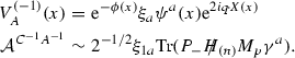
Note that the vertex of an RR in an asymmetric picture has been first proposed by [49] so the vertices can be read off as follows:

$$\begin{aligned}&V_{\phi }^{(0)}(x)=\xi _{1i}(\partial ^i X(x)+i\alpha 'k.\psi \psi ^i(x))\mathrm{e}^{\alpha 'ik.X(x)},\\&V_{\mathrm{RR}}^{(-2)}(z,\bar{z})=(P_{-}C\!\!\!\!/\,_{(n-1)}M_p)^{\alpha \beta }\mathrm{e}^{-3\phi (z)/2},\\&\quad S_{\alpha }(z)\mathrm{e}^{i\frac{\alpha '}{2}p{\cdot }X(z)}\mathrm{e}^{-\phi (\bar{z})/2} S_{\beta }(\bar{z}) \mathrm{e}^{i\frac{\alpha '}{2}p{\cdot }D {\cdot }X(\bar{z})}. \end{aligned}$$

We are considering the disk level amplitude so the RR has to be put in the middle of the disk, while the scalar field needs to be replaced just in its boundary. On-shell conditions for scalar and RR are⁶

$$\begin{aligned} k^2=p^2=0, \quad k.\xi _1=0. \end{aligned}$$

For simplicity it is really useful to just make use of the world-sheet’s holomorphic elements, which means that we employ some useful change of variables as follows:

$$\begin{aligned}&\tilde{X}^{\mu }(\bar{z}) \rightarrow D^{\mu }_{\nu }X^{\nu }(\bar{z}), \ \ \ \tilde{\psi }^{\mu }(\bar{z}) \rightarrow D^{\mu }_{\nu }\psi ^{\nu }(\bar{z}), \ \ \ \tilde{\phi }(\bar{z}) \rightarrow \phi (\bar{z}),\\&\quad \ \ \ \text{ and }\ \ \ \tilde{S}_{\alpha }(\bar{z}) \rightarrow M_{\alpha }{}^{\beta }{S}_{\beta }(\bar{z}). \end{aligned}$$

Some definitions might be important to highlight as well.⁷

Applying those vertex operators and the Wick theorem, our desired S-matrix can be written down:

$$\begin{aligned}&\int \mathrm{d}x_1 \mathrm{d}x_4 \mathrm{d}x_5 (P_{-}C\!\!\!\!/\,_{(n-1)}M_p)^{\alpha \beta } (x_{45})^{-3/4} \xi _{1i}\\&\quad \times \, (I_1+(2i k_{1a})I_2) I, \end{aligned}$$

so that $x_4=z=x+iy,x_5=\bar{z}=x-iy$ and

$$\begin{aligned} I=|x_{14}x_{15}|^{\frac{\alpha '^2}{2}k_1.p} |x_{45}|^{\frac{\alpha '^2}{4}p.D.p}, \end{aligned}$$

(3)

with

$$\begin{aligned} I_1= ip^{i}(x_{54})^{-5/4} C^{-1}_{\alpha \beta }\frac{x_{54}}{x_{14}x_{15} }. \end{aligned}$$

(4)

It is also important to address the following correlator, which can be obtained by generalising the Wick-like rule [50, 51]:

$$\begin{aligned} I_2= & {} \langle :S_{\alpha }(x_4): S_{\beta }(x_5):\psi ^{a}\psi ^{i}(x_1): \rangle \\= & {} 2^{-1}(x_{14}x_{15})^{-1}(x_{45})^{-1/4}(\Gamma ^{ia} C^{-1})_{\alpha \beta }. \end{aligned}$$

If we would replace the above correlators inside the amplitude then we could see that our S-matrix does respect the SL(2, R) invariance. We gauge fix it as $(x_1,z,\bar{z})=(\infty ,i,-i)$, so that the final result of our S-matrix in this certain picture is

(5)

As can be seen from the above S-matrix, it seems to have two different terms in our amplitude, while below we show that some crucial subtleties are needed. Note that after the derivation of the S-matrix, one could start writing all its field theory couplings to be compared with the amplitude, while before doing so, we claim that one has to know the correct form of the S-matrix. Hence let us carry out this amplitude in the other picture $\langle C^{(-1)}\phi ^{(-1)} \rangle$ in the next section and get back to the subtlety associated to Eq. (5) afterwards.

It is also worth to derive the S-matrix of one RR and a gauge field in the asymmetric picture of an RR.⁸

3 The $C^{-1}- \phi ^{-1}$ amplitude

The three point function from the world-sheet perspective (two point function from the space-time point of view) of one RR and a real tachyon of type II super string in their different pictures has been done.⁹

This three point function from the world-sheet perspective with both RR and scalar field in the $(-1)$ picture is given by

$$\begin{aligned} {\mathcal A}^{\phi ,\mathrm{RR}}\sim & {} \int \mathrm{d}x\mathrm{d}^2z \langle V_\phi ^{(-1)}(x) V_{\mathrm{RR}}^{(-1)}(z,\bar{z})\rangle . \end{aligned}$$

(6)

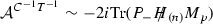
The vertices are written down so that an RR is considered in terms of its field strength in the symmetric picture. They are presented as follows:

$$\begin{aligned}&V_\phi ^{(-1)}(x)=\mathrm{e}^{-\phi (x)}\xi _i\psi ^i(x)\mathrm{e}^{2iq\!\cdot \!X(x)}, \\&V_{\mathrm{RR}}^{(-1)}(z,\bar{z})=(P_{-}H\!\!\!\!/\,_{(n)}M_p)^{\alpha \beta }\mathrm{e}^{-\phi (z)/2},\\&\quad S_{\alpha }(z)\mathrm{e}^{i\frac{\alpha '}{2}p{\cdot }X(z)}\mathrm{e}^{-\phi (\bar{z})/2} S_{\beta }(\bar{z}) \mathrm{e}^{i\frac{\alpha '}{2}p{\cdot }D {\cdot }X(\bar{z})}. \end{aligned}$$

Obviously all the previous definitions of the first section for projector, holomorphic components and the other field contents have been kept here as well. Once more we substitute the defined vertex operators into Eq. (6) and the amplitude reduces to

$$\begin{aligned}&\int \mathrm{d}x_1 \mathrm{d}x_4 \mathrm{d}x_5 (P_{-}H\!\!\!\!/\,_{(n)}M_p)^{\alpha \beta }(x_{14}x_{15})^{-1/2} (x_{45})^{-1/4} \xi _{1i} I\\&\quad \times \langle :S_{\alpha }(x_4): S_{\beta }(x_5):\psi ^{i}(x_1): \rangle \end{aligned}$$

where the result for the following correlation function is needed:

$$\begin{aligned}&\langle :S_{\alpha }(x_4): S_{\beta }(x_5):\psi ^{i}(x_1):\rangle =2^{-1/2}(x_{14}x_{15})^{-1/2}\\&\quad (x_{45})^{-3/4}(\gamma ^{i} C^{-1})_{\alpha \beta }. \end{aligned}$$

The SL(2, R) invariance of the S-matrix can be readily checked and we did gauge fixing as $(\infty ,i,-i)$.¹⁰ The final result of the S-matrix of one scalar and one RR closed string in this symmetric picture is

(7)

One should pay particular attention to the conservation of momentum along the world volume of the brane as $k_1^{a} + p^{a} =0$. Let us first reproduce the field theory of the above S-matrix. The amplitude might be normalised by a coefficient of $(2^{1/2}\pi \mu _p/8)$ such that $\mu _p$ is the Ramond–Ramond charge of the brane. The trace is done as follows¹¹:

Eventually this S-matrix (7) can be precisely produced with the following field theory coupling:

(8)

where we have used the so-called Taylor expansion of a scalar field; meanwhile, in the other picture, the S-matrix was found to be

Let us compare Eq. (5) with (7). We know that $p^i C=H^i$, so up to a normalisation constant the first term of Eq. (5) does exactly produce the same S-matrix as the one of Eq. (7); therefore we claim that the second term of Eq. (5) has no contribution to the S-matrix of one scalar and one RR at all. Hence the prescription for removing or getting rid of the second term of Eq. (5) is as follows.

We first apply the momentum conservation along the world volume of the brane to the second term ($k_1^{a} + p^{a} =0$) and then extract its trace as follows:

and more importantly, in order to get to the same S-matrix as ${\mathcal A}^{\phi ^{-1},C^{-1}}$, we understand that the following Bianchi identity must hold for the BPS branes:

$$\begin{aligned} p^a\epsilon ^{a_{0}\cdots a_{p-1}a} =0. \end{aligned}$$

(9)

However, this is not the full story; as we will see in the next sections for the higher point functions of string amplitudes, one has to generalise all the Bianchi identities.¹² Let us now turn to some of the four point functions and obtain new Bianchi identities.

4 The $T^{-1}-\phi ^{0}-C^{-1}$ amplitude

The four point function from the world-sheet perspective (three point function from the space-time point of view) of one closed string RR and two real tachyons of type II super string with their all different pictures can been done.¹³

The four point function of one tachyon, a scalar and one RR from the world-sheet point of view has been performed in detail in [48]. Indeed both the S-matrix and its field theory part in the following picture $T^{0}-\phi ^{-1}-C^{-1}$ have already been computed. Truly, after carrying out the gauge fixing as $(x_1,x_2,z,\bar{z})=(x,-x,i,-i)$ the S-matrix is given by¹⁴

$$\begin{aligned}&4k_{1a} \xi _i\int _{-\infty }^{\infty } \mathrm{d}x (2x)^{-2u-1/2} ((1+x^{2}))^{-1/2 +2 u}\\&\quad (\text{ Tr }(P_{-}H\!\!\!\!/\,_{(n)}M_p\Gamma ^{ia})). \end{aligned}$$

Thus the result of this non-supersymmetric amplitude is read off as

$$\begin{aligned}&{\mathcal A}^{T^{0},\phi ^{-1},C^{-1}}=(\pi \beta '\mu _p')2\sqrt{\pi } \frac{\Gamma [-u+1/4]}{\Gamma [3/4-u]}\nonumber \\&\quad \text{ Tr }(P_{-}H\!\!\!\!/\,_{(n)}M_p\Gamma ^{ai})k_{1a}\xi _i\text{ Tr }(\lambda _1\lambda _2), \end{aligned}$$

(11)

where $(\pi \beta '\mu _p'/2)$, $\beta '$ and $\mu _p'$ are defined as normalisation constants, WZ and the RR charge of the brane. In effective field theory it was shown that this S-matrix can be precisely reproduced by the following coupling of type II string theory:

$$\begin{aligned} 2i\beta '\mu '_p (2\pi \alpha ')^2\int _{\Sigma _{p+1}} (\text{ Tr }(\partial _{i}C_{p}\wedge DT\phi ^i)), \end{aligned}$$

(12)

and all its infinite corrections were derived in [48].¹⁵

Let us carry it out in the other picture so if we use the above vertex operators and perform all the correlators with the same techniques as have been explained in the previous section, then one explores the final form of the S-matrix in this picture thus:

$$\begin{aligned}&{\mathcal A}^{C^{-1}\phi ^{0}T^{-1}} \sim 4 \xi _{1i}\int _{-\infty }^{\infty } \mathrm{d}x (2x)^{-2u-1/2} ((1+x^{2}))^{2u-1/2} \nonumber \\&\quad \times \, [k_{1a}\text{ Tr }(P_{-}H\!\!\!\!/\,_{(n)}M_p\Gamma ^{ia})-p^i\text{ Tr }(P_{-}H\!\!\!\!/\,_{(n)}M_p)]. \end{aligned}$$

(14)

Now in order to get to the same S-matrix element for this four point world-sheet amplitude as appeared in Eq. (11), one has to apply the momentum conservation $(k_1+k_2+p)^a=0$ and keep in mind the following Bianchi identity as well:

$$\begin{aligned} p^i \epsilon ^{a_{0}...a_{p}}H_{a_{0}...a_{p}}+p^a \epsilon ^{a_{0}...a_{p-1}a}H^{i}_{a_{0}...a_{p-1}}= & {} 0. \end{aligned}$$

(15)

Finally let us calculate this S-matrix in an asymmetric picture of an RR and make some essential comments about this four point function.

Notice that there is a non-zero coupling between two gauge fields and one RR in the world volume of BPS branes of type II string theory.¹⁶

5 The $T^{0}-\phi ^{0}-C^{-2}$ amplitude

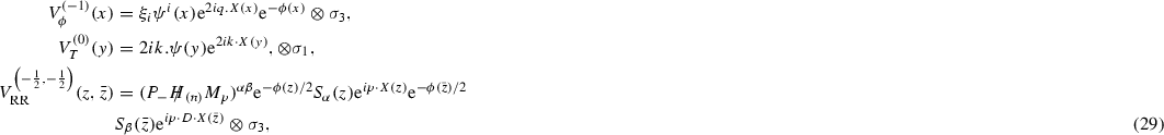
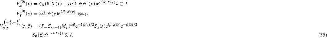
The four point function of an asymmetric RR, a scalar and an open string tachyon can be investigated by the following correlation function:

$$\begin{aligned} {\mathcal A}^ {T^{0}\phi ^{0}C^{-2}}\sim & {} \int \mathrm{d}x_1 \mathrm{d}x_2 \mathrm{d}^2z \langle V_\phi ^{(0)}(x_1)V_T^{(0)}(x_2) V_{\mathrm{RR}}^{(-2)}(z,\bar{z})\rangle \nonumber \\ \end{aligned}$$

(16)

where the tachyon, scalar field and RR vertex operators are given as¹⁷

$$\begin{aligned}&V_{T}^{(0)}(y)=\alpha 'ik_1{\cdot }\psi (y) \mathrm{e}^{\alpha 'ik_1{\cdot }X(y)}\lambda \otimes \sigma _1 ,\\&V_{\phi }^{(0)}(x)=\xi _{1i}(\partial ^i X(x)+i\alpha 'k.\psi \psi ^i(x))\mathrm{e}^{\alpha 'ik.X(x)}\lambda \otimes I ,\\&V_{\mathrm{RR}}^{(-2)}(z,\bar{z})=(P_{-}C\!\!\!\!/\,_{(n-1)}M_p)^{\alpha \beta }\mathrm{e}^{-3\phi (z)/2} S_{\alpha }(z)\mathrm{e}^{i\frac{\alpha '}{2}p{\cdot }X(z)}\\&\quad \mathrm{e}^{-\phi (\bar{z})/2}S_{\beta }(\bar{z}) \mathrm{e}^{i\frac{\alpha '}{2}p{\cdot }D {\cdot }X(\bar{z})}\lambda \otimes \sigma _3\sigma _1. \end{aligned}$$

Applying the Wick theorem, the amplitude can be explored as follows:

$$\begin{aligned}&\int \mathrm{d}x_1 \mathrm{d}x_2 \mathrm{d}x_4 \mathrm{d}x_5 (P_{-}C\!\!\!\!/\,_{(n-1)}M_p)^{\alpha \beta } (x_{45})^{-3/4} (4ik_{2a}) \xi _{1i}\\&\quad \times \, (I_3+(2i k_{1c})I_4) I_5 \end{aligned}$$

with

$$\begin{aligned} I_5= & {} |x_{12}|^{\alpha '^2 k_1.k_2}|x_{14}x_{15}|^{\frac{\alpha '^2}{2}k_1.p} |x_{24}x_{25}|^{\frac{\alpha '^2}{2}k_2.p}|x_{45}|^{\frac{\alpha '^2}{4}p.D.p},\nonumber \\ I_3= & {} ip^{i} 2^{-1/2} (x_{24}x_{25})^{-1/2} (x_{45})^{-3/4} (\gamma ^a C^{-1})_{\alpha \beta }\frac{x_{54}}{x_{14}x_{15} }.\nonumber \\ \end{aligned}$$

(17)

Now using Wick-like rule one gets to the following correlator:

$$\begin{aligned} I_4= & {} \langle :S_{\alpha }(x_4): S_{\beta }(x_5):\psi ^{c}\psi ^{i}(x_1):\psi ^{a}(x_2):\rangle \\= & {} 2^{-3/2}(x_{24}x_{25})^{-1/2}(x_{14}x_{15})^{-1}(x_{45})^{1/4} \\&\times \,\bigg [(\Gamma ^{aic} C^{-1})_{\alpha \beta } +2 \frac{\mathrm{Re}[x_{14}x_{25}]}{x_{12}x_{45}}\eta ^{ac}(\gamma ^{i} C^{-1})_{\alpha \beta }\bigg ]. \end{aligned}$$

By applying the above correlators to this four point amplitude we can easily observe that the integrand or S-matrix is SL(2, R) invariant. We do the proper gauge fixing as $(x_1,x_2,z,\bar{z})=(x,-x,i,-i)$, and taking $u=- \frac{\alpha '}{2} (k_1+k_2)^2$ we obtain the S-matrix as

$$\begin{aligned} {\mathcal A}^{T^{0}\phi ^{0}C^{-2}}={\mathcal A}_1+\mathcal{A}_2, \end{aligned}$$

such that

$$\begin{aligned}&{\mathcal A}_{1}^{T^{0}\phi ^{0}C^{-2}}=2^{3/2}\xi _{1i} k_{2a} p^i \text{ Tr }(C\!\!\!\!/\,_{(n-1)}M_p \gamma ^{a})\nonumber \\&\qquad \times \int _{-\infty }^{\infty } (2x)^{-2t-1/2} (x^2+1)^{2t-1/2}\nonumber \\&\quad = 2^{3/2}\xi _{1i} 4k_{2a} p^i \text{ Tr }(C\!\!\!\!/\,_{(n-1)}M_p \gamma ^{a})\sqrt{\pi } \frac{\Gamma [-u+1/4]}{\Gamma [3/4-u]}.\nonumber \\ \end{aligned}$$

(18)

Now if we use the momentum conservation $(k_1+k_2+p)^a=0$ and the Bianchi identity $p^a\epsilon ^{a_{0}\cdots a_{p-1}a} =0$, then we come to the point that up to a coefficient of $2^{3/2}$ this part of the S-matrix exactly produces (11). The second part of the S-matrix is found to be

$$\begin{aligned}&{\mathcal A}_{2}^{T^{0}\phi ^{0}C^{-2}}=2^{3/2}\xi _{1i} k_{1c} k_{2a} \int _{-\infty }^{\infty } (2x)^{-2t-1/2} (x^2+1)^{2t-1/2}\nonumber \\&\quad \times \bigg [2\eta ^{ac}\text{ Tr }(C\!\!\!\!/\,_{(n-1)}M_p \gamma ^{i})\frac{1-x^2}{4xi}+\text{ Tr }(C\!\!\!\!/\,_{(n-1)}M_p \Gamma ^{aic})\bigg ]\nonumber \\ \end{aligned}$$

(19)

where the first term in (19) is indeed zero, because the integration is taken over the whole space, while the integrand is odd, so naturally the answer for the first term of Eq. (19) is zero¹⁸

However, clearly, the result for the second term of Eq. (19) is non-zero, that is,

$$\begin{aligned} {\mathcal A}_{2}^{T^{0}\phi ^{0}C^{-2}}= & {} 2^{3/2}\xi _{1i} 4k_{1c} k_{2a} \text{ Tr }(C\!\!\!\!/\,_{(n-1)}M_p\Gamma ^{aic})\nonumber \\&\times \,\sqrt{\pi } \frac{\Gamma [-u+1/4]}{\Gamma [3/4-u]}. \end{aligned}$$

(21)

Therefore we might think of this term as the extra contact interaction to the S-matrix; however, after applying momentum conservation along the world volume of the brane and using Bianchi identities,¹⁹ it becomes clear for us that this term has a zero contribution to the S-matrix of an asymmetric RR, a scalar and a tachyon.²⁰

6 The $\phi ^{0}-A^{0}-C^{-2}$ amplitude

The four point function of an asymmetric RR, a scalar and a gauge field can be carried out by the following correlation function:

$$\begin{aligned} {\mathcal A}^ {\phi ^{0} A^{0}C^{-2}}\sim & {} \int \mathrm{d}x_1 \mathrm{d}x_2 \mathrm{d}^2z \langle V_\phi ^{(0)}(x_1)V_A^{(0)}(x_2) V_{\mathrm{RR}}^{(-2)}(z,\bar{z})\rangle \nonumber \\ \end{aligned}$$

(22)

where the scalar field and RR vertex operators are given in the previous sections, and for the gauge field we have

$$\begin{aligned} V_{A}^{(0)}(x)= & {} \xi _{2a}(\partial ^a X(x)+i\alpha 'k.\psi \psi ^a(x))\mathrm{e}^{\alpha 'ik.X(x)}. \end{aligned}$$

Having set the Wick theorem, the amplitude may have been written down as

$$\begin{aligned}&\int \mathrm{d}x_1 \mathrm{d}x_2 \mathrm{d}x_4 \mathrm{d}x_5 (P_{-}C\!\!\!\!/\,_{(n-1)}M_p)^{\alpha \beta } (x_{45})^{-3/4} \xi _{1i}\xi _{2a}\\&\quad \times (J_1+J_2+J_3+J_4) I_5 \end{aligned}$$

and also

$$\begin{aligned} I_5= & {} |x_{12}|^{\alpha '^2 k_1.k_2}|x_{14}x_{15}|^{\frac{\alpha '^2}{2}k_1.p} |x_{24}x_{25}|^{\frac{\alpha '^2}{2}k_2.p}|x_{45}|^{\frac{\alpha '^2}{4}p.D.p},\nonumber \\ \end{aligned}$$

(23)

where by applying the generalisation of a Wick-like rule one can obtain all the correlators as follows:

$$\begin{aligned} J_1= & {} ip^{i}\frac{x_{54}}{x_{14}x_{15}} (l_a) (x_{45})^{-5/4} ( C^{-1})_{\alpha \beta }\nonumber \\ l_a= & {} -ik_{1a}\bigg [\frac{x_{14}}{x_{12}x_{24}}+\frac{x_{15}}{x_{12}x_{25}}\bigg ]\nonumber \\ J_2= & {} -p^{i}k_{2c}\frac{x_{54}}{x_{14}x_{15}} (x_{24}x_{25})^{-1} (x_{45})^{-1/4} ( \Gamma ^{ac}C^{-1})_{\alpha \beta }\nonumber \\ J_3= & {} (l_a) ik_{1b} (x_{14}x_{15})^{-1} (x_{45})^{-1/4} ( \Gamma ^{ib}C^{-1})_{\alpha \beta }\nonumber \\ J_4= & {} -k_{1b}k_{2c} (x_{14}x_{15}x_{24}x_{25})^{-1} (x_{45})^{3/4} \nonumber \\&\times \bigg [ ( \Gamma ^{acib}C^{-1})_{\alpha \beta }+(2\eta ^{bc}(\Gamma ^{ai}C^{-1})_{\alpha \beta }\nonumber \\&-2\eta ^{ab}(\Gamma ^{ci}C^{-1})_{\alpha \beta })\frac{\mathrm{Re}[x_{14}x_{25}]}{x_{12}x_{45}}\bigg ]. \end{aligned}$$

(24)

If we now apply Eq. (24) into this four point amplitude we can easily determine that the S-matrix is SL(2, R) invariant. We do the proper gauge fixing as $(x_1,x_2,z,\bar{z})=(x,-x,i,-i)$, taking $t=- \frac{\alpha '}{2} (k_1+k_2)^2$ to actually get to the entire S-matrix as

$$\begin{aligned}&{\mathcal A}^{\phi ^{0}A^{0}C^{-2}}=-\xi _{1i}\xi _{2a}\int _{-\infty }^{\infty }\mathrm{d}x (1+x^2)^{2t-1} (2x)^{-2t}\nonumber \\&\quad \bigg [\frac{1-x^2}{x}(-ip^i k_{1a}\text{ Tr }(P_{-}C\!\!\!\!/\,_{(n-1)}M_p)\nonumber \\&\quad \quad +k_{1b}k_{1a}\text{ Tr }(P_{-}C\!\!\!\!/\,_{(n-1)}M_p\Gamma ^{ib}) \nonumber \\&\quad \quad +\,\eta ^{bc}\text{ Tr }(P_{-}C\!\!\!\!/\,_{(n-1)}M_p\Gamma ^{ai})\nonumber \\&\quad \quad -\,\eta ^{ab}\text{ Tr }(P_{-}C\!\!\!\!/\,_{(n-1)}M_p\Gamma ^{ci}))\nonumber \\&\quad \quad +\,2ik_{2c}p^i\text{ Tr }(P_{-}C\!\!\!\!/\,_{(n-1)}M_p\Gamma ^{ac}) \nonumber \\&\quad \quad -\,2ik_{1b}k_{2c}\text{ Tr }(P_{-}C\!\!\!\!/\,_{(n-1)}M_p\Gamma ^{acib})\bigg ] \end{aligned}$$

(25)

where the first, second, third and fourth term do not make any contribution to the S-matrix because the integration is taken on the whole space and the integrand is odd. If we use the momentum conservation $(k_1+k_2+p)^a=0$ and the Bianchi identity $p_b\epsilon ^{a_{0}\cdots a_{p-3}bac} =0$, then we see that the sixth term makes also no contribution to the amplitude, so only the fifth term has a non-zero contribution to the S-matrix of an asymmetric RR, a scalar and a gauge field.

Hence, the final result is

$$\begin{aligned}&{\mathcal A}^{\phi ^{0}A^{0}C^{-2}}=-\xi _{1i}\xi _{2a} 2ik_{2c}p^i\text{ Tr }(P_{-}C\!\!\!\!/\,_{(n-1)}M_p\Gamma ^{ac}) \pi ^{1/2}\nonumber \\&\quad \times \, \frac{\Gamma [-t+1/2]}{\Gamma [1-t]} \end{aligned}$$

(26)

where the expansion of the amplitude is non-zero for the $p=n$ case and it does not include any poles as is clear from Eq. (26), because the low energy expansion is the $t\rightarrow 0$ limit and all the infinite contact interactions of this S-matrix have already been derived in [43]. Given the closed form of the above correlation functions one can find ${\mathcal A}^{\phi ^{-1}A^{0}C^{-1}}$ as well;

$$\begin{aligned} {\mathcal A}^{\phi ^{-1}A^{0}C^{-1}}= & {} 2^{-3/2}\xi _{1i}\xi _{2a}\int _{-\infty }^{\infty }\mathrm{d}x (1+x^2)^{2t-1} (2x)^{-2t}\\&\times \,\bigg [\frac{1-x^2}{x}(k_{1a}\text{ Tr }(P_{-}H\!\!\!\!/\,_{(n)}M_p\gamma ^i)\\&-2ik_{2b}\text{ Tr }(P_{-}H\!\!\!\!/\,_{(n)}M_p\Gamma ^{abi})\bigg ] \end{aligned}$$

where again the first term makes no contribution and the second term (up to a coefficient of $2^{3/2}$) precisely produces (26). Finally one explores this amplitude in its last picture as follows:

$$\begin{aligned} {\mathcal A}^{\phi ^{0}A^{-1}C^{-1}}= & {} 2^{1/2}\xi _{1i}\xi _{2a}\int _{-\infty }^{\infty }\mathrm{d}x (1+x^2)^{2t-1} (2x)^{-2t}\nonumber \\&\times [k_{1b}\text{ Tr }(P_{-}H\!\!\!\!/\,_{(n)}M_p\Gamma ^{bai})\nonumber \\&-p^i\text{ Tr }(P_{-}H\!\!\!\!/\,_{(n)}M_p\gamma ^{a})] \end{aligned}$$

(27)

where in Eq. (27), one has to apply momentum conservation to its first term and use the Bianchi identity

$$\begin{aligned} p_b\epsilon ^{a_{0}\cdots a_{p-2}ba} H^i_{a_{0}\cdots a_{p-2}}+p^i\epsilon ^{a_{0}\cdots a_{p-1}a} H_{a_{0}\cdots a_{p-1}}= & {} 0 \end{aligned}$$

(28)

to actually get to the entire S-matrix as appeared in (26).

Therefore in this particular picture, again we are just left with one term for the final answer of the RR, a gauge and a scalar field and this term is necessary because this S-matrix has to be produced by a non-zero coupling, $(2\pi \alpha ')^2\mu _p\int _{H^{+}}\partial _{i}C_{a_{0}..a_{p-2}}, F_{a_{p-1}a_{p}} \phi ^i$ of effective field theory where the scalar field comes from a Taylor expansion.

Note that by comparing this S-matrix with field theory, we begin to understand that there should not be any other term in effective field theory coming from the pull-back of the brane.

Now in order to obtain the other non-trivial Bianchi identities, we are going to consider one of the simplest five point functions and deal with more subtleties as regards perturbative string theory.

7 The five point world-sheet S-matrix of the brane–anti-brane system

It is known that the world volume of the brane–anti-brane system must have two real tachyon fields.²¹ The complete form of the amplitude of a gauge, two real tachyons and an RR of a brane–anti-brane system for the various p, n cases $\langle V_{A}^{(-1)}{(x_{1})} V_{T}^{(0)}{(x_{2})}V_T^{(0)}{(x_{3})} V_{RR}^{(-\frac{1}{2},-\frac{1}{2})}(z,\bar{z})\rangle$ has been derived in [54].

For completeness we have done this amplitude in the following picture as well:

$$\begin{aligned} \langle V_{A}^{(0)}{(x_{1})} V_{T}^{(-1)}{(x_{2})}V_T^{(0)}{(x_{3})} V_{\mathrm{RR}}^{(-\frac{1}{2},-\frac{1}{2})}(z,\bar{z})\rangle , \end{aligned}$$

and the final result for the amplitude is exactly the same as appeared in [54] so that it satisfies the Ward identity associated to the gauge field. It is also worth explaining that the S-matrix elements of one RR field, one scalar field and two tachyons on the world volume brane–anti-brane system in the following picture have also been computed in detail in [55]²²

$$\begin{aligned} \langle V_{\phi }^{(-1)}{(x_{1})} V_{T}^{(0)}{(x_{2})}V_T^{(0)}{(x_{3})} V_{\mathrm{RR}}^{\left( -\frac{1}{2},-\frac{1}{2}\right) }(z,\bar{z})\rangle . \end{aligned}$$

(31)

The final form of this S-matrix in this particular picture is given as

$$\begin{aligned} {\mathcal A}^{C^{(-1)}\phi ^{(-1)} T^{(0)} T^{(0)}}= & {} {\mathcal A}_{1}+{\mathcal A}_{2} \end{aligned}$$

(32)

where

(33)

where $L_1,L_2$ are written down below just in terms of Gamma functions (no hypergeometric function is needed):

$$\begin{aligned}&L_1=(2)^{-2(t+s+u)-1}\pi \nonumber \\&\quad \times \, {\frac{\Gamma (-u) \Gamma (-s+\frac{1}{4})\Gamma (-t+\frac{1}{4})\Gamma (-t-s-u)}{\Gamma (-u-t+\frac{1}{4})\Gamma (-t-s+\frac{1}{2})\Gamma (-s-u+\frac{1}{4})}},\nonumber \\&L_2=(2)^{-2(t+s+u+1)}\pi \nonumber \\&\quad \times \, {\frac{\Gamma (-u+\frac{1}{2}) \Gamma (-s+\frac{3}{4})\Gamma (-t+\frac{3}{4})\Gamma (-t-s-u-\frac{1}{2})}{\Gamma (-u-t+\frac{1}{4})\Gamma (-t-s+\frac{1}{2})\Gamma (-s-u+\frac{1}{4})}}\nonumber \\ \end{aligned}$$

(34)

where in [55] all the infinite u channel gauge poles of $L_1$ and the $t+s'+u'$ channel scalar poles of this S-matrix have been precisely produced, in addition to all the infinite higher derivative corrections to two scalars–two tachyons of the world volume of the brane–anti-brane, which have also without any ambiguity been discovered.

Now let us deal with this S-matrix in the other pictures of both closed–open strings to see what happens to the complete form of the S-matrix and also explore all its contact interactions.

8 $C^{(-2)} \phi ^{(0)} T^{(0)} T^{(0)}$

The S-matrix element of an asymmetric RR field, one scalar field and two tachyons on the world volume of the brane–anti-brane system can be found as follows.²³ Replacing the vertex operators and performing all the correlators by using the Wick theorem, one can investigate the whole of the amplitudes as follows:

$$\begin{aligned}&{\mathcal A}^{C^{(-2)} \phi ^{(0)} T^{(0)} T^{(0)}} \sim \int \mathrm{d}x_{1}\mathrm{d}x_{2}\mathrm{d}x_{3}\mathrm{d}x_{4} \mathrm{d}x_{5}\, (P_{-}C\!\!\!\!/\,_{(n-1)}M_p)^{\alpha \beta }\nonumber \\&\xi _{1i}x_{45}^{-3/4}( -8 k_{2b}k_{3c}) I \bigg (\bigg (ip^i \frac{x_{54}}{x_{15}x_{14}}\bigg )I_1^{cb}+2i k_{1a}I_2^{cbia}\bigg )\nonumber \\ \end{aligned}$$

(36)

where $x_{ij}=x_i-x_j$,

$$\begin{aligned} I= & {} |x_{12}|^{4k_1.k_2}|x_{13}|^{4k_1.k_3}|x_{14}x_{15}|^{2k_1.p}|x_{23}|^{4k_2.k_3}\nonumber \\&\times \, |x_{24}x_{25}|^{2k_2.p}|x_{34}x_{35}|^{2k_3.p}|x_{45}|^{p.D.p}. \end{aligned}$$

(37)

Note that we have already generalised the Wick theorem to get to the fermionic correlations in the presence of currents so that one can find the following correlators:

$$\begin{aligned} I_1^{cb}= & {} \langle :S_{\alpha }(x_4):S_{\beta }(x_5):\psi ^b(x_2)::\psi ^c(x_3): \rangle \\= & {} 2^{-1}x_{45}^{-1/4} (x_{24}x_{25}x_{34}x_{35})^{-1/2}\\&\times \bigg ((\Gamma ^{cb}C^{-1})_{\alpha \beta }-2\eta ^{bc}\frac{\mathrm{Re}[x_{24}x_{35}]}{x_{23}x_{45}}(C^{-1})_{\alpha \beta }\bigg ) \end{aligned}$$

and also

$$\begin{aligned} I_2^{cbia}= & {} \langle :S_{\alpha }(x_4):S_{\beta }(x_5):\psi ^a \psi ^i(x_1):\psi ^b(x_2)::\psi ^c(x_3):\rangle \\&=2^{-2}x_{45}^{3/4} (x_{24}x_{25}x_{34}x_{35})^{-1/2} (x_{14}x_{15})^{-1}\\&\quad \times \, \bigg \{(\Gamma ^{cbia}C^{-1})_{\alpha \beta } +2\eta ^{ab}\frac{\mathrm{Re}[x_{14}x_{25}]}{x_{12}x_{45}}(\Gamma ^{ci}C^{-1})_{\alpha \beta }\\&\quad \quad -2\eta ^{ac}\frac{\mathrm{Re}[x_{14}x_{35}]}{x_{13}x_{45}}(\Gamma ^{bi}C^{-1})_{\alpha \beta }\\&\quad \quad -2\eta ^{bc}\frac{\mathrm{Re}[x_{24}x_{35}]}{x_{23}x_{45}}(\Gamma ^{ia}C^{-1})_{\alpha \beta } \bigg \}. \end{aligned}$$

If we substitute all the above correlations in the amplitude, then one can show that the property of SL(2, R) invariance is in order in our investigation. Here we are working with a five point function and to the best of our knowledge the best gauge fixing for this amplitude is to fix the locations of all three open strings as follows:

$$\begin{aligned} x_{1}=0 ,\quad x_{2}=1,\quad x_{3}\rightarrow \infty . \end{aligned}$$

If we do so, then we get the entire form of the S-matrix in terms of some integrations on the upper half plane, so that the following integrations for various cases need to be performed:

$$\begin{aligned} \int \mathrm{d}^2 \!z |1-z|^{a} |z|^{b} (z - \bar{z})^{c} (z + \bar{z})^{d}, \end{aligned}$$

(38)

with $d=0,1,2$, and a, b, c must be just given in terms of the Mandelstam variables. Notice that the result of the above integrations for $d=0,1$ is got from [54, 56], while for $d=2$ the result is given in [13, 14].

If we do gauge fixing, make use of various pure algebraic simplifications and most particularly make use of the results of the integrals that are pointed out in [13, 14, 54, 56] then we can write down the final result of the amplitude (36) in this asymmetric picture as follows:

$$\begin{aligned} {\mathcal A}^{C^{-2}\phi ^{0} T^{0} T^{0}}= & {} {\mathcal A}_{1}+{\mathcal A}_{2}+{\mathcal A}_{3}+{\mathcal A}_{4} \end{aligned}$$

(39)

where

$$\begin{aligned} {\mathcal A}_{1}&\!\!\!\sim \!\!\!&ip^i\xi _{1i}(4 k_{2b}k_{3c}) \text{ Tr }(P_{-}C\!\!\!\!/\,_{(n-1)}M_p\Gamma ^{cb})L_1, \nonumber \\ {\mathcal A}_{2}\sim & {} 4i p^i \xi _{1i} \{\text{ Tr }(P_{-}C\!\!\!\!/\,_{(n-1)}M_p)\} L_2, \nonumber \\ {\mathcal A}_{3}\sim & {} -4i \xi _{1i} k_{1a}k_{2b}k_{3c} \{\text{ Tr }(P_{-}C\!\!\!\!/\,_{(n-1)}M_p \Gamma ^{cbia})\} L_1, \nonumber \\ {\mathcal A}_{4}\sim & {} 4i \xi _{1i} \{\text{ Tr }(P_{-}C\!\!\!\!/\,_{(n-1)}M_p\Gamma ^{bi})\} L_2 (k_{1b}+k_{2b}+k_{3b})\nonumber \\ \end{aligned}$$

(40)

where the functions $L_1,L_2$ are given in (34).

Note that here in (40) we have dealt with the five point world-sheet scattering of the brane–anti-brane in an asymmetric picture and in this particular picture we found the terms that carry momentum of an RR in the transverse directions. These terms no longer vanish and indeed these terms potentially have something to do with some of the issues on the perturbative string theory on the upper half plane. We believe that these terms are related to taking the integration on different moduli space as has been pointed out in a series of papers [44–47].

Now if we compare the S-matrix in this asymmetric picture (40) with (33), then we might think of the fact that the last two terms of Eq. (40) are extra singularities. Indeed if we do not apply the Bianchi identity and momentum conservation along the brane to (40) as a matter of fact these two terms would be extra terms by themselves. However, if we compare (40) with (33), simultaneously extract the trace in the last term of Eq. (40) and make use of the momentum conservation along the world volume of the brane as follows:

$$\begin{aligned} (k_1+k_2+k_3)^a= & {} -p^a, \end{aligned}$$

(41)

we come to the conclusion that the last term in (40) is an apparent singularity and this should be removed, in the other words, upon applying the Bianchi identity

$$\begin{aligned} p^b\epsilon ^{a_{0}\cdots a_{p-1}b}C^{i}_{a_{0}\cdots a_{p-1}}=0 \end{aligned}$$

(42)

the last term of Eq. (40) vanishes.

Note that below we show that the above Bianchi identity cannot be applied to the correlators,

$$\begin{aligned} \langle V_{T}^{(0)}{(x_{1})}V_{T}^{(0)}{(x_{2})}V_T^{(0)}{(x_{3})} V_{\mathrm{RR}}^{\left( -\frac{3}{2},-\frac{1}{2}\right) }(z,\bar{z})\rangle , \end{aligned}$$

of non-BPS branes. Indeed after gauge fixing, $(x_1,x_2,z,\bar{z})=(0,1,\infty ,z,\bar{z})$, we obtain the following non-BPS amplitude:

$$\begin{aligned}&{\mathcal A}^{C^{-2}T^{0} T^{0} T^{0}}= -16i (2^{-3/2} k_{1a} k_{2b} k_{3c})(P_{-}C\!\!\!\!/\,_{(n)}M_p)^{\alpha \beta }\\&\quad \int \mathrm{d}^2z |1-z|^{2t+2u} |z|^{2t+2s} (z - \bar{z})^{-2(t+s+u+1)}\\&\quad \times \bigg [(\Gamma ^{cba} C^{-1})_{\alpha \beta }+\frac{(z + \bar{z})}{2(z - \bar{z})}\\&\quad \times \, ((2\eta ^{ac}(\gamma ^b C^{-1})_{\alpha \beta })-(2\eta ^{ab}(\gamma ^c C^{-1})_{\alpha \beta })\\&\quad -(2\eta ^{bc}(\gamma ^a C^{-1})_{\alpha \beta })) +(2\eta ^{bc}(\gamma ^a C^{-1})_{\alpha \beta })\frac{1}{(z - \bar{z})}\\&\quad +(2\eta ^{ab}(\gamma ^c C^{-1})_{\alpha \beta })\frac{|z|^{2}}{(z - \bar{z})}\bigg ]. \end{aligned}$$

We make use of various pure algebraic simplifications to write down the final result for the above amplitude in this asymmetric picture as follows:

$$\begin{aligned} {\mathcal A}^{C^{-2}T^{0} T^{0} T^{0}}= & {} {\mathcal A}_{1}+{\mathcal A}_{2} \end{aligned}$$

where

$$\begin{aligned} {\mathcal A}_{1}&\!\!\!\sim \!\!\!&-16i (2^{-3/2} k_{1a} k_{2b} k_{3c})\text{ Tr }(P_{-}C\!\!\!\!/\,_{(n-1)}M_p\Gamma ^{cba})N_1\\ {\mathcal A}_{2}\sim & {} -16i (2^{-3/2})\text{ Tr }(P_{-}C\!\!\!\!/\,_{(n-1)}M_p\gamma ^{a})N_2 (k_{1a}+k_{2a}+k_{3a}) \end{aligned}$$

where the functions $N_1,N_2$ are given as

$$\begin{aligned}&N_1=(2)^{-2(t+s+u+1)}\pi \nonumber \\&\quad {\frac{\Gamma (-u) \Gamma (-s)\Gamma (-t)\Gamma \left( -t-s-u-\frac{1}{2}\right) }{\Gamma (-u-t)\Gamma (-t-s)\Gamma (-s-u)}},\nonumber \\&N_2=(2)^{-2(t+s+u)-3}\pi \nonumber \\&\quad {\frac{\Gamma \left( -u+\frac{1}{2}\right) \Gamma \left( -s+\frac{1}{2}\right) \Gamma \left( -t+\frac{1}{2}\right) \Gamma (-t-s-u-1)}{\Gamma (-u-t)\Gamma (-t-s)\Gamma (-s-u)}}.\nonumber \\ \end{aligned}$$

(43)

Note that if we use momentum conservation $p^a=-(k_1+k_2+k_3)^a$ for both the first and the second part of the above non-BPS S-matrix we see that

$$\begin{aligned}&p^a\epsilon ^{a_{0}\cdots a_{p-3}cba}C_{a_{0}\cdots a_{p-3}}, p^c\epsilon ^{a_{0}\cdots a_{p-3}cba}C_{a_{0}\cdots a_{p-3}},\\&\quad p^a\epsilon ^{a_{0}\cdots a_{p-1}a}C_{a_{0}\cdots a_{p-1}} \end{aligned}$$

are not zero. In particular in order to make sense of non-supersymmetric amplitudes in the world volume of non-BPS branes, the equations

$$\begin{aligned} p^a\epsilon ^{a_{0}\cdots a_{p-3}cba},\quad p^a\epsilon ^{a_{0}\cdots a_{p-1}a} \end{aligned}$$

(44)

must be non-zero.

Hence for non-supersymmetric amplitudes first we must extract the traces and keep in mind the above points, that is, the equations that we found for some of the BPS branes cannot be applied to non-BPS amplitudes in the presence of a scalar field and an RR. Indeed we expect to see that behaviour because the equations that hold for the BPS cases not necessarily obtain for the non-supersymmetric cases, whereas for the BPS branes the equations seem to be more manifest, while this may have been changed after symmetry breaking. The lesson is that for scattering of the mixed scalars–tachyons in the presence of an RR (in its asymmetric picture), one needs to break several identities that necessary hold for BPS branes.

What about the third term of Eq. (40)? One might add it to the first term of Eq. (40) and find that

$$\begin{aligned} k_{2b}k_{3c}\xi _{1i}(p^i\epsilon ^{a_{0}\cdots a_{p-2}cb}C_{a_{0}\cdots a_{p-2}}+p^a\epsilon ^{a_{0}\cdots a_{p-3}cba}C^{i}_{a_{0}\cdots a_{p-3}}) \end{aligned}$$

should vanish; however, from (33) we know that the first term of Eq. (40) holds and plays a crucial role in effective field theory. Thus we need to explore a new Bianchi identity for the third term of Eq. (40). In fact if we actually apply momentum conservation to the third term of Eq. (40) and because of the antisymmetric property of $\epsilon$ we conclude that the equation $p^a\epsilon ^{a_{0}\cdots a_{p-3}cba}C^{i}_{a_{0}\cdots a_{p-3}}$ must vanish for brane–anti-brane amplitudes.

Therefore, the lesson we have learnt is as follows. In the presence of an asymmetric RR, a scalar and some tachyons, one needs to find new Bianchi identities to get the same S-matrix elements as obtained by a symmetric RR, a scalar and some tachyons. This is because we have no gauge field to check the gauge invariance of the amplitude and, more accurately, there is no Ward identity for the scalar field.

Now let us address the same S-matrix of a symmetric RR, two tachyons and a scalar field in the zero picture, $\langle C^{(-1)} \phi ^{(0)} T^{(-1)} T^{(0)} \rangle$.

9 $C^{(-1)} \phi ^{(0)} T^{(-1)} T^{(0)}$

Finally this S-matrix element of a symmetric RR field, one scalar in the zero picture and two tachyons on the world volume of the brane–anti-brane system can be written down:

$$\begin{aligned}&{\mathcal A}^ {C^{(-1)} \phi ^{(0)} T^{(-1)} T^{(0)}} \sim \int \mathrm{d}x_1 \mathrm{d}x_2 \mathrm{d}x_3 \mathrm{d}^2z\\&\quad \times \langle V_{\phi }^{(0)}{(x_{1})} V_{T}^{(-1)}{(x_{2})}V_T^{(0)}{(x_{3})} V_{\mathrm{RR}}^{\left( -\frac{1}{2},-\frac{1}{2}\right) }(z,\bar{z})\rangle \end{aligned}$$

with the following vertices

$$\begin{aligned}&V_{T}^{(-1)}(y) = \mathrm{e}^{-\phi (y)} \mathrm{e}^{2ik{\cdot }X(y)} \otimes \sigma _2\nonumber \\&V_{\mathrm{RR}}^{\left( -\frac{1}{2},-\frac{1}{2}\right) }(z,\bar{z})=(P_{-}H\!\!\!\!/\,_{(n)}M_p)^{\alpha \beta }\mathrm{e}^{-\phi (z)/2}\nonumber \\&\quad S_{\alpha }(z)\mathrm{e}^{ip{\cdot }X(z)}\mathrm{e}^{-\phi (\bar{z})/2} S_{\beta }(\bar{z}) \mathrm{e}^{ip{\cdot }D {\cdot }X(\bar{z})}\otimes \sigma _3; \end{aligned}$$

(45)

we just write down the amplitude in its compact form as

$$\begin{aligned}&{\mathcal A}^{C^{(-1)} \phi ^{(0)} T^{(-1)} T^{(0)}} \sim \int \mathrm{d}x_{1}\mathrm{d}x_{2}\mathrm{d}x_{3}\mathrm{d}x_{4} \mathrm{d}x_{5}\\&(P_{-}H\!\!\!\!/\,_{(n)}M_p)^{\alpha \beta }\xi _{1i}( 4 k_{3b}) x_{45}^{-1/4}(x_{24}x_{25})^{-1/2}I \\&\quad \times \bigg (\bigg (ip^i \frac{x_{54}}{x_{15}x_{14}}\bigg )I_1^{b}+2i k_{1a}I_2^{bia}\bigg ) \end{aligned}$$

where $x_{ij}=x_i-x_j$,

$$\begin{aligned}&I=|x_{12}|^{4k_1.k_2}|x_{13}|^{4k_1.k_3}|x_{14}x_{15}|^{2k_1.p}|x_{23}|^{4k_2.k_3}\\&\quad \times |x_{24}x_{25}|^{2k_2.p}|x_{34}x_{35}|^{2k_3.p}|x_{45}|^{p.D.p} \end{aligned}$$

where the following correlators need to be replaced inside the amplitude

$$\begin{aligned} I_1^{b}= & {} \langle :S_{\alpha }(x_4):S_{\beta }(x_5):\psi ^b(x_3):\rangle \\= & {} 2^{-1/2}x_{45}^{-3/4} (x_{34}x_{35})^{-1/2}(\gamma ^{b}C^{-1})_{\alpha \beta } \end{aligned}$$

and also

$$\begin{aligned} I_2^{bia}= & {} \langle :S_{\alpha }(x_4):S_{\beta }(x_5):\psi ^a \psi ^i(x_1):\psi ^b(x_3):\rangle \\= & {} 2^{-3/2}x_{45}^{1/4} (x_{34}x_{35})^{-1/2} (x_{14}x_{15})^{-1}\\&\times \bigg \{(\Gamma ^{bia}C^{-1})_{\alpha \beta }+2\eta ^{ab}\frac{\mathrm{Re}[x_{14}x_{35}]}{x_{13}x_{45}}(\gamma ^{i}C^{-1})_{\alpha \beta }\bigg \}. \end{aligned}$$

Notice that, given the above correlations, one may easily investigate the SL(2, R) transformation of the S-matrix. We performed gauge fixing by just fixing the location of the open strings so that the final integration needs to be done over the closed string RR ’s position on the upper half complex plane.²⁴

Once more after gauge fixing one finds the same sort of integration as we discussed earlier on.²⁵

Having calculated all the desired integrals, one could explore the result for the S-matrix in its particular picture as follows:

$$\begin{aligned} {\mathcal A}^{C^{(-1)} \phi ^{(0)} T^{(-1)} T^{(0)}}= & {} {\mathcal A}_{1}+{\mathcal A}_{2}+{\mathcal A}_{3} \end{aligned}$$

(47)

in such a way that all its components are given by

$$\begin{aligned} {\mathcal A}_{1}&\!\!\!\sim \!\!\!&-2i 2^{1/2} p^i\xi _{1i}k_{3b} \text{ Tr }(P_{-}H\!\!\!\!/\,_{(n)}M_p\gamma ^{b})L_1, \nonumber \\ {\mathcal A}_{2}\sim & {} -2i 2^{1/2}\xi _{1i} \{\text{ Tr }(P_{-}H\!\!\!\!/\,_{(n)}M_p \Gamma ^{bia})\}k_{1a} k_{3b} L_1 \nonumber \\ {\mathcal A}_{3}\sim & {} -2i 2^{1/2}\xi _{1i} \{\text{ Tr }(P_{-}H\!\!\!\!/\,_{(n)}M_p \gamma ^{i})\} L_2 \end{aligned}$$

(48)

where the $L_1,L_2$ functions are already given in (34). If we compare (48) with (33), then we might wonder whether the first term of ${\mathcal A}^{C^{(-1)} \phi ^{(0)} T^{(-1)} T^{(0)}}$ is an extra term, because it is also related to all infinite singularities. However, it is worthwhile pointing out that we have already produced all the infinite u channel gauge poles by taking into account the second term of Eq. (48). Therefore one has to find or generalise new Bianchi identities to actually remove the first extra term of Eq. (48). Hence we apply momentum conservation, $k_{1a}=-k_{2a}-k_{3a}-p_{a}$, to the second term of (48), extract the traces, use the antisymmetric property of the $\epsilon$ tensor and eventually add the first and second components of the amplitude to derive the following Bianchi identity:

$$\begin{aligned}&\xi _{1i} k_{3b}(-p_a\epsilon ^{a_{0}\cdots a_{p-2}ab}H^{i}_{a_{0}\cdots a_{p-2}}\nonumber \\&\quad +p^i\epsilon ^{a_{0}\cdots a_{p-1}b}H_{a_{0}\cdots a_{p-1}})=0. \end{aligned}$$

(49)

Thus by holding (49) and keeping in mind momentum conservation along the world volume of the brane we are precisely able to obtain the same S-matrix as appeared in (33), so we find the following crucial fact as regards this five point function of the brane–anti-brane system.

If we consider an RR in the asymmetric picture $C^{-3/2,-1/2}$ and a scalar field in the zero picture with some other open string tachyons then we must find all new Bianchi identities to be able to remove all the extra apparent singularities of asymmetric picture of the brane–anti-brane systems.

In the next section we will reveal some features for non-BPS branes to actually restore the Ward identity associated (gauge invariance) to the gauge field and also we derive all the precise contact interactions of mixed RR, scalar/gauge and tachyon string amplitudes. Namely we show that if we consider the scalar field in the zero picture and the RR in an asymmetric picture $(C^{-3/2,-1/2})$ then in this particular case there is no need to explore new Bianchi identities to the S-matrix of non-BPS amplitudes and more importantly those amplitudes independently respect the Ward identity associated to the gauge field.

10 $C^{-1}\phi ^{0}A^{-1}T^{0}$ S-matrix

In [48] the five point world-sheet amplitude of a symmetric RR with one scalar, a gauge field and a tachyon in the world volume of non-BPS branes of type II string theory $\langle C^{-1}\phi ^{-1}A^{0}T^{0} \rangle$ was achieved and all the correlators were found.²⁶

The final result in this symmetric picture was read off as

$$\begin{aligned} {\mathcal A}^{C^{-1}\phi ^{-1}A^{0}T^{0}}= & {} {\mathcal A}_{1}+{\mathcal A}_{2} \end{aligned}$$

(51)

where

$$\begin{aligned} {\mathcal A}_{1}&\!\!\!\sim \!\!\!&2\xi _{1i}\xi _{2a}k_{3c}k_{2d} \text{ Tr }(P_{-}H\!\!\!\!/\,_{(n)}M_p\Gamma ^{cadi} )L_1', \nonumber \\ {\mathcal A}_{2}\sim & {} (2L_3')\{-t\text{ Tr }(P_{-}H\!\!\!\!/\,_{(n)}M_p \gamma .\xi _2\gamma .\xi _{1})u'\nonumber \\&-2tk_3.\xi _2\text{ Tr }(P_{-}H\!\!\!\!/\,_{(n)}M_p \gamma .k_2\gamma .\xi _{1}) \nonumber \\&+\text{ Tr }(P_{-}H\!\!\!\!/\,_{(n)}M_p \gamma .k_3\gamma .\xi _{1})(-2t(k_3.\xi _2)+2u'k_1.\xi _2)\}.\nonumber \\ \end{aligned}$$

(52)

It was also shown that one needs to use the momentum conservation, $s+t+u=-p^ap_a-\frac{1}{4}$, applying $t \rightarrow 0, s \rightarrow -\frac{1}{4}, u \rightarrow -\frac{1}{4}$ to the S-matrix to be able to derive all infinite $u',t$ channel tachyon and scalar poles of the non-super symmetric amplitudes accordingly. Note that $L_1'$ has just infinite contact interactions.

It is of high importance to note that this particular ${\mathcal A}^{C^{-1}\phi ^{-1}A^{0}T^{0}}$ amplitude does respect all the symmetries and most importantly it does satisfy the Ward identity associated to the gauge field. Indeed if we replace $\xi _{2a}\rightarrow k_{2a}$ inside (52), then the first term of Eq. (52) is automatically zero because

$$\begin{aligned} k_{2a} k_{2d} k_{3c} \epsilon ^{a_{0}\cdots a_{p-2}cad}=0; \end{aligned}$$

replacing $\xi _{2a}\rightarrow k_{2a}$ inside the second, third, fourth and fifth term of Eq. (52) we also get a zero result for the whole S-matrix²⁷ so gauge invariance is satisfied. Thus based on just replacing $\xi _{2a}\rightarrow k_{2a}$ of the gauge field, the whole S-matrix vanishes.

Having explained all the needed ingredients of the S-matrices, in the following we would like to change the vertex of the scalar field and see what happens to the gauge invariance of a mixture of five point world-sheet amplitudes of a symmetric RR with one scalar in the zero picture, a gauge field and a tachyon in the world volume of non-BPS branes of type II string theory. This $\langle C^{-1}\phi ^{0}A^{-1}T^{0} \rangle$ amplitude is given by the following correlation functions:

$$\begin{aligned}&{\mathcal A}^{C^{-1}\phi ^{0}A^{-1}T^{0}} \sim \int \mathrm{d}x_{1}\mathrm{d}x_{2}\mathrm{d}x_{3}\mathrm{d}z\mathrm{d}\bar{z}\,\nonumber \\&\quad \times \langle V_{\phi }^{(0)}{(x_{1})}V_{A}^{(-1)}{(x_{2})}V_T^{(0)}{(x_{3})} V_{\mathrm{RR}}^{\left( -\frac{1}{2},-\frac{1}{2}\right) }(z,\bar{z})\rangle . \end{aligned}$$

(53)

Let us write down the rest of the vertex operators, including their CP factors,

$$\begin{aligned} V_{A}^{(-1)}(y)= & {} \xi _{2a}\psi ^a(y)\mathrm{e}^{\alpha 'iq.X(y)}\mathrm{e}^{-\phi (y)}\otimes \sigma _3 ,\nonumber \\ V_{\phi }^{(0)}(x)= & {} \xi _{1i}(\partial ^i X(x)+i\alpha 'k.\psi \psi ^i(x))\mathrm{e}^{\alpha 'ik.X(x)}\otimes I \end{aligned}$$

(54)

where the on-shell conditions for scalar, gauge, RR and tachyon hold.²⁸

Once more we deal with just the holomorphic elements of all fields involving $X^{\mu }\psi ^\mu , \phi$, so that the S-matrix is now given by

$$\begin{aligned}&{\mathcal A}^{C^{-1}\phi ^{0}A^{-1}T^{0}} \sim \int \mathrm{d}x_{1}\mathrm{d}x_{2}\mathrm{d}x_{3}\mathrm{d}x_{4} \mathrm{d}x_{5}\, (P_{-}H\!\!\!\!/\,_{(n)}M_p)^{\alpha \beta }\nonumber \\&\quad \times \, \xi _{1i}\xi _{2a}(\alpha 'ik_{3c})x_{45}^{-1/4}(x_{24}x_{25})^{-1/2}\nonumber \\&\quad \times \, (I_1+I_2)I\text{ Tr }(\lambda _1\lambda _2\lambda _3)\text{ Tr }(\sigma _3\sigma _1I\sigma _3\sigma _1), \end{aligned}$$

(55)

where²⁹ $x_{ij}=x_i-x_j$. Let us find all the fermionic and bosonic correlators:

$$\begin{aligned}&I_1=\langle :\partial X^i{(x_1)}\mathrm{e}^{\alpha 'ik_1.X(x_1)}: \mathrm{e}^{\alpha 'ik_2.X(x_2)}:\mathrm{e}^{\alpha 'ik_3.X(x_3)}\nonumber \\&\quad :\mathrm{e}^{\frac{\alpha '}{2}ip.X(x_4)}:\mathrm{e}^{\frac{\alpha '}{2}ip.D.X(x_5)}: \rangle \nonumber \\&\quad \times {\langle :S_{\alpha }(x_4):S_{\beta }(x_5):\psi ^a(x_2):\psi ^c(x_3) \rangle },\nonumber \\&I_2=\langle :\mathrm{e}^{\alpha 'ik_1.X(x_1)}: \mathrm{e}^{\alpha 'ik_2.X(x_2)}:\mathrm{e}^{\alpha 'ik_3.X(x_3)}\nonumber \\&\quad :\mathrm{e}^{\frac{\alpha '}{2}ip.X(x_4)}:\mathrm{e}^{\frac{\alpha '}{2}ip.D.X(x_5)}: \rangle \nonumber \\&\quad \alpha 'ik_{1d} {\langle :S_{\alpha }(x_4):S_{\beta }(x_5):\psi ^d\psi ^{i}(x_1):\psi ^a(x_2)::\psi ^c(x_3):\rangle }.\nonumber \\ \end{aligned}$$

(57)

We need to use the Wick-like rule [50] to get all the generalisations of the correlation functions of two spin and two fermion operators such as the following:

$$\begin{aligned} I_5^{ca}= & {} \langle :S_{\alpha }(x_4):S_{\beta }(x_5):\psi ^a(x_2):\psi ^c(x_3):\rangle \\= & {} 2^{-1}x_{45}^{-1/4} (x_{24}x_{25}x_{34}x_{35})^{-1/2}\\&\times \,\bigg \{(\Gamma ^{ca}C^{-1})_{\alpha \beta }-2\frac{\mathrm{Re}[x_{24}x_{35}]}{x_{23}x_{45}}\eta ^{ac}(C^{-1})_{{\alpha \beta }}\bigg \}. \end{aligned}$$

Now we need to make use of [12] to obtain the final answer of the correlation function in ten dimensions,

$$\begin{aligned}&I_6^{caid}=\langle :S_{\alpha }(x_4):S_{\beta }(x_5):\psi ^d\psi ^{i}(x_1):\psi ^a(x_2)::\psi ^c(x_3):\rangle \nonumber \\&\quad =\bigg \{(\Gamma ^{caid}C^{-1})_{{\alpha \beta }}+\frac{\mathrm{Re}[x_{14}x_{25}]}{x_{12}x_{45}}(2\eta ^{da}(\Gamma ^{ci}C^{-1})_{{\alpha \beta }})\nonumber \\&\qquad -2\frac{\mathrm{Re}[x_{14}x_{35}]}{x_{13}x_{45}}\eta ^{dc}(\Gamma ^{ai}C^{-1})_{{\alpha \beta }}\nonumber \\&\qquad -2\frac{\mathrm{Re}[x_{24}x_{35}]}{x_{23}x_{45}}\eta ^{ac}(\Gamma ^{id}C^{-1})_{{\alpha \beta }}\bigg \} 2^{-2}x_{45}^{3/4}\nonumber \\&\quad \quad \times \,(x_{24}x_{25}x_{34}x_{35})^{-1/2}(x_{14}x_{15})^{-1}. \end{aligned}$$

(58)

Now we are allowed to replace all the correlators inside (55) to obtain the compact form of the desired S-matrix as follows:

$$\begin{aligned}&{\mathcal A}^{C^{-1}\phi ^{0}A^{-1}T^{0}} \!\!\!\!\sim \!\! \int \mathrm{d}x_{1}\mathrm{d}x_{2} \mathrm{d}x_{3}\mathrm{d}x_{4}\mathrm{d}x_{5}(P_{-}H\!\!\!\!/\,_{(n)}M_p)^{\alpha \beta }I\xi _{1i}\xi _{2a}\nonumber \\&\quad \times \, (-2\alpha 'ik_{3c}) x_{45}^{-1/4}(x_{24}x_{25})^{-1/2}\nonumber \\&\quad \times \, (a^i_2 I_5^{ca} +\alpha 'ik_{1d}I_6^{caid})\text{ Tr }(\lambda _1\lambda _2\lambda _3), \end{aligned}$$

(59)

so that

$$\begin{aligned} a^i_2= & {} ip^{i}\bigg (\frac{x_{54}}{x_{14}x_{15}}\bigg ). \end{aligned}$$

(60)

We are now able to investigate whether the amplitude satisfies the SL(2, R) invariance, and we also did gauge fixing by just fixing the positions of three open strings.³⁰

The solutions for all the integrals on the upper half plane have been released and the ultimate result of the S-matrix will be obtained as

$$\begin{aligned} {\mathcal A}^{C^{-1}\phi ^{0}A^{-1}T^{0}}= & {} {\mathcal A}_{1}+{\mathcal A}_{2}, \end{aligned}$$

(63)

where

$$\begin{aligned}&{\mathcal A}_{1} \!\sim \! (2\xi _{1i}\xi _{2a}k_{3c}k_{1d} \text{ Tr }(P_{-}H\!\!\!\!/\,_{(n)}M_p\Gamma ^{caid})\nonumber \\&\quad -\xi _1.p(2k_{3c}\xi _{2a}) \text{ Tr }(P_{-}H\!\!\!\!/\,_{(n)}M_p\Gamma ^{ca}) )L_1',\nonumber \\&{\mathcal A}_{2} \sim \bigg \{t\xi _1.p (4k_{3}.\xi _2)\text{ Tr }(P_{-}H\!\!\!\!/\,_{(n)}M_p )\nonumber \\&\quad +\, 4\left( u+\frac{1}{4}\right) k_{3c}\xi _{1i}\text{ Tr }(P_{-}H\!\!\!\!/\,_{(n)}M_p\Gamma ^{ci})k_1.\xi _2\nonumber \\&\quad -\,4tk_{3}.\xi _{2} k_{1b}\xi _{1i}\text{ Tr }(P_{-}H\!\!\!\!/\,_{(n)}M_p\Gamma ^{ib})\nonumber \\&\quad -2t\left( u+\frac{1}{4}\right) \xi _{1i}\xi _{2a}\text{ Tr }(P_{-}H\!\!\!\!/\,_{(n)}M_p\Gamma ^{ai}) \bigg \}L_3'. \end{aligned}$$

(64)

Note that we have already analysed all infinite $u'$ tachyon and massless t channel scalar poles of the amplitude in [48].

In this picture after replacing $\xi _{2a}\rightarrow k_{2a}$ (due to the terms $\xi _1.p$) the amplitude does not satisfy the Ward identity associated to the gauge field and indeed the second and third terms would remain whereas $L_3'$ cannot be removed by $L_1'$. Let us compare the result of this amplitude (63) with (52) to make a statement on mixed closed and open string amplitudes including one scalar and one RR and some other open tachyons. The last term in (64) is exactly the second term of Eq. (52), the fourth term in (64) is exactly the last term of Eq. (52). Note that if we add the third and fourth term of (52) and use the momentum conservation along the world volume of the brane, then the result is precisely equivalent with the fifth term of Eq. (64). Once more by using momentum conservation in the world volume direction the first term of Eq. (64) is exactly equivalent with the first term in (52).

However, the second and the third terms of Eq. (64) are extra terms and in particular if we use anti-commutator relation of $\gamma$ matrices these two terms cannot cancel each other due to the fact that $L_3'$ is different from $L_1'$.

Indeed if we replace $\xi _{2a}\rightarrow k_{2a}$ inside (64) and use momentum conservation along the brane, the first term is automatically zero because

$$\begin{aligned} k_{2a} k_{3c} k_{1d} \epsilon ^{a_{0}\cdots a_{p-2}cad}=0 \end{aligned}$$

By replacing $\xi _{2a}\rightarrow k_{2a}$ inside the fourth, fifth and sixth terms of Eq. (64) appropriately we also get zero result as follows

$$\begin{aligned} -2tu' \xi _{1i} (k_{2a}+ k_{1a}+k_{3a})\epsilon ^{a_{0}\cdots a_{p-1}a}=0 \end{aligned}$$

Thus the second and third terms give rise the amplitude not to be gauge invariant unless one finds some new Bianchi identities.³¹

In the next section we show that by considering the asymmetric RR and a scalar, a gauge and one tachyon in the zero picture of non-BPS branes, the S-matrix automatically satisfies a Ward identity without the need to introduce any new Bianchi identities.

10.1 $C^{-2}\phi ^{0}A^{0}T^{0}$ S-matrix

One can do the same CFT methods to actually derive the entire S-matrix of the above strings in the asymmetric picture. Hence the final answer for the five point world-sheet amplitude of a RR (in an asymmetric picture) with one scalar, a gauge field and a tachyon in the world volume of non-BPS branes of type II string theory $\langle C^{-2}\phi ^{0}A^{0}T^{0} \rangle$ is

$$\begin{aligned} {\mathcal A}^{C^{-2}\phi ^{0}A^{0}T^{0}}= & {} {\mathcal A}_{1}+{\mathcal A}_{2}+{\mathcal A}_{3}+{\mathcal A}_{4} \end{aligned}$$

(66)

where

$$\begin{aligned}&{\mathcal A}_{1} \sim 2^{3/2}i\xi _{1i}\xi _{2a}k_{3c}k_{2b}L_1' (p^i\text{ Tr }(P_{-}C\!\!\!\!/\,_{(n)}M_p\Gamma ^{cab})\nonumber \\&\qquad \quad -k_{1d}\text{ Tr }(P_{-}C\!\!\!\!/\,_{(n)}M_p\Gamma ^{cabid}) \nonumber \\&{\mathcal A}_{2} \sim 2^{3/2}i\xi _1.p L_3' \text{ Tr }(P_{-}C\!\!\!\!/\,_{(n)}M_p \gamma ^c)(2tk_3.\xi _2 [-k_{3c}-k_{2c}]\nonumber \\&\quad \quad +2k_1.\xi _2u'k_{3c}-tu'\xi _{2c})\nonumber \\&{\mathcal A}_{3} \sim 2^{3/2}i\xi _{1i}L_3' \text{ Tr }(P_{-}C\!\!\!\!/\,_{(n)}M_p \Gamma ^{cid})\nonumber \\&\qquad \quad \times \,[-2k_1.\xi _2 u'k_{3c}(k_{1d}+k_{2d})+2tk_3.\xi _2 k_{1d}(k_{3c}+k_{2c})] \nonumber \\&{\mathcal A}_{4} \sim 2^{3/2}i\xi _{1i}L_3't u' \xi _{2a} \text{ Tr }(P_{-}C\!\!\!\!/\,_{(n)}M_p \Gamma ^{cai})\nonumber \\&\qquad \quad \times \,(k_{3c}+k_{1c}+k_{2c}) \end{aligned}$$

(67)

with $u'=(-u-\frac{1}{4})$ and the same introduced $L_1',L_3'$. $L_1'$ has infinite contact interactions and $L_3'$ has infinite $t,u'$ scalar–tachyon channel poles accordingly.

The nice thing about this asymmetric S-matrix is that without introducing any further Bianchi identity this amplitude automatically satisfies the Ward identity associated to the gauge field, which means that if we replace $\xi _{2a}\rightarrow k_{2a}$ the whole S-matrix vanishes where the following points are needed. In the first term of ${\mathcal A}_{2}$ one has to apply momentum conservation along the world volume of the brane $-k_{3c}-k_{2c}=p_c+k_{1c}$ and apply the following identity:

$$\begin{aligned} p_c \epsilon ^{a_{0}...a_{p-1}c}= & {} 0. \end{aligned}$$

We need to apply momentum conservation in ${\mathcal A}_{3}$’s first term, that is, $-k_{1d}-k_{2d}=p_d+k_{3d}$ and then draw particular attention to the fact that this part of the S-matrix involves $k_{3d} k_{3c}\epsilon ^{a_{0}...a_{p-2}dc} C^{i}_{a_{0}...a_{p-2}}$, which is zero because of the antisymmetric property of the $\epsilon$ tensor. Likewise, we need to replace $k_{3c}+k_{2c}=-p_c-k_{1c}$ and $k_{1d} k_{1c}\epsilon ^{a_{0}...a_{p-2}dc} C^{i}_{a_{0}...a_{p-2}}=0$. Finally, we apply momentum conservation to the last term of Eq. (67) and note that $p_c \epsilon ^{a_{0}...a_{p-2}ca} C^{i}_{a_{0}...a_{p-2}}=0$ plays the crucial role in checking the Ward identity.

The last remark about the asymmetric picture of the S-matrices is that one finds all the entire contact interactions of string theory amplitudes properly. For instance this amplitude includes several contact interaction terms like the first term and the last terms of Eq. (67), which could be missed in its symmetric picture of (64).

11 Conclusion

We have derived scattering amplitudes of all three, four and five point BPS and non-BPS mixture of a closed string Ramond–Ramond, a scalar field, gauge and tachyons in all their different pictures of both world volume and transverse directions (for the general p, n cases) of type IIA (IIB) string theory.

In particular we have shown that if we carry out the calculations of higher point functions in an asymmetric picture of Ramond–Ramond (taking its vertex operator in terms of its potential $C^{-2}$) and scalar field in the zero picture, then various equations must be kept fixed for BPS branes, the entire contact interactions can be definitely obtained and, most importantly, the Ward identity associated to the gauge field is also satisfied.

More accurately, by direct calculations on the upper half plane, we have also observed that some of the Bianchi identities (which must be true) for BPS branes cannot be necessarily applied to non-BPS amplitudes, otherwise the whole S-matrix might vanish. Indeed in the presence of the scalar field and RR, the terms carrying momentum of an RR in the transverse directions $(p^i,p^j)$ play an important role in the entire form of the S-matrix and one has to keep them in five point functions.

We expect it to be true for higher point functions of string theory amplitudes and it would be nice to check it directly. It would also be important to deal with some other subtleties of perturbative string theory [44–47].

References

J. Polchinski, Dirichlet branes and Ramond–Ramond charges. Phys. Rev. Lett. 75, 4724 (1995). arXiv:hep-th/9510017
E. Witten, Bound states of strings and p-branes. Nucl. Phys. B 460, 335 (1996). arXiv:hep-th/9510135
J. Polchinski, Tasi lectures on D-branes. arXiv:hep-th/9611050
R.C. Myers, Dielectric branes. JHEP 9912, 022 (1999). arXiv:hep-th/9910053
E. Hatefi, A.J. Nurmagambetov, I.Y. Park, \(N^3\) entropy of \(M5\) branes from dielectric effect. Nucl. Phys. B 866, 58 (2013).arXiv:1204.2711 [hep-th]
C. Bachas, D-Brane dynamics. Phys. Lett. B 374, 37 (1996). arXiv:hep-th/9511043
M. Li, Boundary states of D-branes and Dy strings. Nucl. Phys. B 460, 351 (1996). arXiv:hep-th/9510161
M.R. Douglas, Branes within branes. In Strings, Branes and Dualities, ed. by Cargese (1997), pp. 267–275. arXiv:hep-th/9512077
M.B. Green, J.A. Harvey, G.W. Moore, I-Brane inflow and anomalous couplings on d-branes. Class. Quant. Grav. 14, 47 (1997). arXiv:hep-th/9605033
D. Junghans, G. Shiu, Brane Curvature Corrections to the \(\cal N =1\) Type II/F-Theory Effective Action. arXiv:1407.0019 [hep-th]
E. Hatefi, Shedding light on new Wess–Zumino couplings with their corrections to all orders in alpha-prime. JHEP 1304, 070 (2013).arXiv:1211.2413 [hep-th]
E. Hatefi, On effective actions of BPS branes and their higher derivative corrections. JHEP 1005, 080 (2010).arXiv:1003.0314 [hep-th]
E. Hatefi, On higher derivative corrections to Wess–Zumino and Tachyonic actions in type II super string theory. Phys. Rev. D 86, 046003 (2012).arXiv:1203.1329 [hep-th]
E. Hatefi, All order \(\alpha ^{\prime }\) higher derivative corrections to non-BPS branes of type IIB super string theory. JHEP 1307, 002 (2013).arXiv:1304.3711 [hep-th]
A. Sen, NonBPS states and branes in string theory. arXiv:hep-th/9904207
N.D. Lambert, H. Liu, J.M. Maldacena, Closed strings from decaying D-branes. JHEP 0703, 014 (2007). arXiv:hep-th/0303139
A. Sen, Tachyon dynamics in open string theory. Int. J. Mod. Phys. A 20, 5513 (2005). arXiv:hep-th/0410103
E. Hatefi, Closed string Ramond–Ramond proposed higher derivative interactions on fermionic amplitudes in IIB. Nucl. Phys. B 880, 1 (2014).arXiv:1302.5024 [hep-th]
E. Hatefi, Super-Yang–Mills, Chern–Simons couplings and their all order \(\alpha ^{\prime }\) corrections in IIB superstring theory. Eur. Phys. J. C 74(8), 3003 (2014). arXiv:1310.8308 [hep-th]
E. Hatefi, SYM, Chern–Simons, Wess–Zumino couplings and their higher derivative corrections in IIA superstring theory. Eur. Phys. J. C 74, 2949 (2014).arXiv:1403.1238 [hep-th]
E. Hatefi, More on Ramond–Ramond, SYM, WZ couplings and their corrections in IIA. Eur. Phys. J. C 74(10), 3116 (2014). arXiv:1403.7167 [hep-th]
L.A. Barreiro, R. Medina, RNS derivation of N-point disk amplitudes from the revisited S-matrix approach. Nucl. Phys. B 886, 870 (2014).arXiv:1310.5942 [hep-th]
L.A. Barreiro, R. Medina, Revisiting the S-matrix approach to the open superstring low energy effective lagrangian. JHEP 1210, 108 (2012).arXiv:1208.6066 [hep-th]
E. Hatefi, I.Y. Park, Universality in all-order \(\alpha ^{\prime }\) corrections to BPS/non-BPS brane world volume theories. Nucl. Phys. B 864, 640 (2012).arXiv:1205.5079 [hep-th]
T. Maxfield, J. McOrist, D. Robbins, S. Sethi, JHEP 1312, 032 (2013). arXiv:1309.2577 [hep-th]
E. Hatefi, A.J. Nurmagambetov, I.Y. Park, Near-extremal black-branes with n*3 entropy growth. Int. J. Mod. Phys. A 27, 1250182 (2012).arXiv:1204.6303 [hep-th]
E. Hatefi, A.J. Nurmagambetov, I.Y. Park, ADM reduction of IIB on \({\cal H}^{p,q}\) to dS braneworld. JHEP 1304, 170 (2013). arXiv:1210.3825 [hep-th]
S. de Alwis, R. Gupta, E. Hatefi, F. Quevedo, Stability, tunneling and flux changing de Sitter transitions in the large volume string scenario. JHEP 1311, 179 (2013). arXiv:1308.1222 [hep-th]
O. Bergman, M.R. Gaberdiel, Stable nonBPS D particles. Phys. Lett. B 441, 133 (1998). arXiv:hep-th/9806155
M. Frau, L. Gallot, A. Lerda, P. Strigazzi, Stable nonBPS D-branes in type I string theory. Nucl. Phys. B 564, 60 (2000). arXiv:hep-th/9903123
E. Dudas, J. Mourad, A. Sagnotti, Charged and uncharged D-branes in various string theories. Nucl. Phys. B 620, 109 (2002). arXiv:hep-th/0107081
E. Eyras, S. Panda, The space-time life of a nonBPS D particle. Nucl. Phys. B 584, 251 (2000). arXiv:hep-th/0003033
E. Eyras, S. Panda, NonBPS branes in a type I orbifold. JHEP 0105, 056 (2001). arXiv:hep-th/0009224
E. Witten, D-Branes and K theory. JHEP 9812, 019 (1998). arXiv:hep-th/9810188
G.R. Dvali, S.H.H. Tye, Brane inflation. Phys. Lett. B 450, 72 (1999). arXiv:hep-ph/9812483
C.P. Burgess, M. Majumdar, D. Nolte, F. Quevedo, G. Rajesh, R.-J. Zhang, The inflationary brane anti-brane universe. JHEP 0107, 047 (2001). arXiv:hep-th/0105204
D. Choudhury, D. Ghoshal, D.P. Jatkar, S. Panda, Hybrid inflation and brane–anti-brane system. JCAP 0307, 009 (2003). arXiv:hep-th/0305104
S. Kachru, R. Kallosh, A.D. Linde, J.M. Maldacena, L.P. McAllister, S.P. Trivedi, Towards inflation in string theory. JCAP 0310, 013 (2003). arXiv:hep-th/0308055
R. Casero, E. Kiritsis, A. Paredes, Chiral symmetry breaking as open string tachyon condensation. Nucl. Phys. B 787, 98 (2007) arXiv:hep-th/0702155 [hep-th]
A. Dhar, P. Nag, Sakai–Sugimoto model, tachyon condensation and chiral symmetry breaking. JHEP 0801, 055 (2008).arXiv:0708.3233 [hep-th]
D. Friedan, E.J. Martinec, S.H. Shenker, Conformal invariance, supersymmetry and string theory. Nucl. Phys. B 271, 93 (1986)
C. Kennedy, A. Wilkins, Ramond–Ramond couplings on brane–anti-brane systems. Phys. Lett. B 464, 206 (1999). arXiv:hep-th/9905195
E. Hatefi, I.Y. Park, More on closed string induced higher derivative interactions on D-branes. Phys. Rev. D 85, 125039 (2012).arXiv:1203.5553 [hep-th]
E. Witten, Superstring Perturbation Theory Revisited. arXiv:1209.5461
E. Witten, Notes on Super Riemann Surfaces and Their Moduli. arXiv:1209.2459
E. Witten, More on Superstring Perturbation Theory. arXiv:1304.2832
E. Witten, Notes on Supermanifolds and Integration. arXiv:1209.2199
E. Hatefi, Selection rules and RR couplings on non-BPS branes. JHEP 1311, 204 (2013).arXiv:1307.3520
M. Bianchi, G. Pradisi, A. Sagnotti, Nucl. Phys. B 376, 365 (1992)
H. Liu, J. Michelson, *-trek III: the search for Ramond–Ramond couplings. Nucl. Phys. B 614, 330 (2001). arXiv:hep-th/0107172
M.R. Garousi, E. Hatefi, More on WZ action of non-BPS branes. JHEP 0903, 008 (2009).arXiv:0812.4216 [hep-th]
E. Hatefi, Three point tree level amplitude in superstring theory. Nucl. Phys. Proc. Suppl. 216, 234 (2011).arXiv:1102.5042 [hep-th]
B. Michel, E. Mintun, J. Polchinski, A. Puhm, P. Saad, Remarks on brane and antibrane dynamics. arXiv:1412.5702 [hep-th]
M.R. Garousi, E. Hatefi, On Wess–Zumino terms of brane–antibrane systems. Nucl. Phys. B 800, 502 (2008).arXiv:0710.5875 [hep-th]
E. Hatefi, On D-brane anti D-brane effective actions and their corrections to all orders in alpha-prime. JCAP 1309, 011 (2013).arXiv:1211.5538, [hep-th]
A. Fotopoulos, On (alpha’)**2 corrections to the D-brane action for non-geodesic world-volume embeddings. JHEP 0109, 005 (2001). arXiv:hep-th/0104146
Acknowledgments
The author would like to thank E. Witten, J. Polchinski, L. Alvarez-Gaume, W. Lerche, R. de Mello Koch, S. Ramgoolam, R. Myers, S. Hirano, V. Jejjala, K. Zoubos, D. Friedan, N. Arkani-Hamed and K.S. Narain for valuable discussions/comments and for their great remarks. Some parts of the computations of this paper were done in Harvard, Institute for advanced study in Princeton, ICTP and CERN, but the final work has been completed in IHES. In particular, the author would like to thank both ICTP and CERN for their great hospitality and their continuous support in his career.
Author information
Authors and Affiliations
Corresponding author
Rights and permissions
Open Access This article is distributed under the terms of the Creative Commons Attribution 4.0 International License (http://creativecommons.org/licenses/by/4.0/), which permits unrestricted use, distribution, and reproduction in any medium, provided you give appropriate credit to the original author(s) and the source, provide a link to the Creative Commons license, and indicate if changes were made.
Funded by SCOAP3
About this article
Cite this article
Hatefi, E. Remarks on the mixed Ramond–Ramond, open string scattering amplitudes of BPS, non-BPS and brane–anti-brane. Eur. Phys. J. C 75, 517 (2015). https://doi.org/10.1140/epjc/s10052-015-3739-4
Received:
Accepted:
Published:
DOI: https://doi.org/10.1140/epjc/s10052-015-3739-4