Preemptive expediting to improve project due date performance

Abstract

Project expediting is often viewed as a corrective action taken in response to prior scheduling errors and is usually applied in the later stages of projects when it appears that predefined due dates will not be met. However, large-scale projects with uncertain activity durations tend to have numerous probabilistic network paths with complex interactions that require some level of expediting to ensure successful scheduling outcomes. Because potential expediting options are consumed over time, delaying expediting efforts until the later stages of projects is likely to result in higher expediting costs or poorer due date performance. This research introduces a preemptive expediting approach that evaluates the probability of completion before the due date throughout the life of a project and selects expediting options per a prespecified probability tolerance or expediting budget. An experiment demonstrates the benefits of this preemptive approach.

Appendix

In each of the experiments the O ₀ matrix is compiled from a randomly generated adjacency matrix per the network type factor settings and the flow diagram in Figure A1 using the following definitions:

E _i :

=set of candidate predecessors for activity i

P _i :

=set of selected predecessors for activity i

f _ik :

∼U(0,1) for activity i in sample k

d _i :

=selection determinant for activity i

n _i :

=goal number of predecessors for activity i

p _ij :

=position of selected candidate for activity i in iteration j

N(i):

=number of activities

N(E _i ):

=number of elements in E _i

N(P _i ):

=number of elements in P _i

Figure A1

Random path generation procedure.

The goal number of predecessors for each activity is randomly determined by a selection determinant (d _i ) that is continually adjusted in order to generate a network based on the network type factor level (d ₀), as follows:

The purpose of Eq. (6) is to handle the competing goals of generating randomly interesting networks and allowing d _i to converge to d ₀. This is accomplished programmatically by defining different probabilities based on the value of d _i . For example, P(n _i <d ₀)=0.95 when d _i <d ₀ and P(n _i >d ₀)=0.95 when d _i >d ₀. Then the predecessors for each activity are randomly determined by iteratively selecting from the set of candidates (sorted in numerical order) as follows:

At each iteration the selected candidate is added to the set of selected predecessors (P _i ) and the set of candidate predecessors (E _i ) is reduced by the selected candidate and all predecessors and successors of the selected candidate per the flow diagram in Figure A1. After completing a number of practice runs with a range of network type factor levels (d ₀) to view the relationship between the factor levels and the resultant networks, levels of 1.05 (sparse) and 1.40 (dense) were chosen for this study because they covered a wide range of network structures.

For demonstration purposes, consider the five-activity adjacency matrix depicted in Table A1. This matrix, which shows the predecessors (In) as the rows and the successors (Out) as the columns for each activity, is initialized with all zeros per step 1 in Figure A1. Defining activity indices in order of precedence similar to Fulkerson (1962) requires only that the portion of the matrix below the diagonal be completed and results in an initial activity (the start event) having no predecessors. Then the process proceeds as follows for each activity:

• 1 E ₁={0}, d ₁=d ₀

  

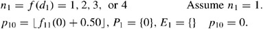
  Candidate predecessor of activity 1 is activity 0 and the selection determinant (d ₁) is set to the network density factor level (d ₀). Activity 1 is randomly determined to have 1 predecessor and activity 0 in position 0 is selected from the set of candidates.

• 2 E ₂={0,1}, d ₂=2d ₀−1

  

  Candidate predecessors of activity 2 are equal to the set E ₂ and the selection determinant (d ₂) is updated per the previous period's results. Activity 2 is randomly determined to have 1 predecessor and activity 0 in position 0 is randomly selected from the set of candidates.

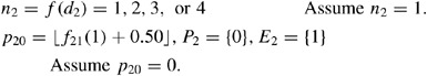
• 3 E ₃={0,1,2}, d ₃=2d ₀−1

  

  Candidate predecessors of activity 3 are equal to the set E ₃ and the selection determinant (d ₃) is updated per the previous errors. Activity 3 is randomly determined to have 2 predecessors. Activity 2 in position 2 is randomly selected from the set of candidates in the first iteration and activity 1 in position 0 is selected in the second iteration.

• 4
  

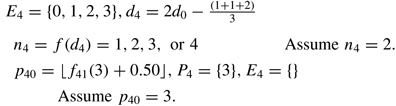
  Candidate predecessors of activity 4 are equal to the set E ₄ and the selection determinant (d ₄) is updated per the previous values. Activity 4 is randomly determined to have 2 predecessors. Activity 3 in position 3 is randomly selected from the set of candidates in the first iteration. The procedure terminates after this iteration because E ₄ becomes a null set.

• 5
  

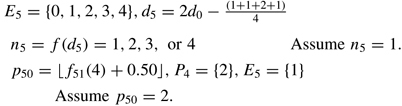
  Candidate predecessors of activity 5 are equal to the set E ₅ and the selection determinant (d ₅) is updated per the previous values. Activity 5 is randomly determined to have 1 predecessor. Activity 2 in position 2 is randomly selected from the set of candidates.

Table 3 Example adjacency matrix

Tracing the predecessor values in the adjacency matrix results in paths 0-1-3-4, 0-2-3-4 and 0-2-5.

References

Baiocchi G (2004). Using Perl for statistics: Data processing and statistical computing. J Stat Software 11: 1–75.
Baker BM (1997). Cost/time tradeoff analysis for the critical path method: A derivation of the network flow approach. J Opl Res Soc 48: 1241–1244.
Bein WW, Kamburowski J and Stallmann MFM (1992). Optimal reduction of two-terminal directed acyclic graphs. SIAM J Comput 21: 1112–1129.
Berman EB (1964). Resource allocation in PERT network under continuous time-cost functions. Mngt Sci 10: 734–745.
Bildson RA and Gillespie JR (1962). Critical path planning—PERT integration. Opns Res 10: 909–912.
Bilstein N and Radermacher FJ (1977). Time-cost optimization. Meth Opns Res 27: 274–294.
Bregman RL (2006). A heuristic procedure for solving the dynamic probabilistic project expediting problem. Working paper, University of Houston.
Cavanaugh J (2001). PDL—The Perl Data Language, version 2.4.2. Available at http://pdl.perl.org.
Christiansen T and Torkington N (2003). Perl Cookbook, 2nd edn. Sebastopol, CA: O'Reilly and Associates.
Clark CE (1961). The optimum allocation of resources among the activities of a network. J Ind Eng 12: 11–17.
Crowston W (1970). Network reduction and solution. Opl Res Quart 21: 435–450.
Crowston W and Thompson GL (1967). Decision CPM: A method for simultaneously planning, scheduling, and control of projects. Opns Res 15: 407–426.
Davis EW (1966). Resource allocation in project network models—a survey. J Ind Eng 17: 177–188.
De P, Dunne EJ, Ghosh JB and Wells CE (1995). The discrete time-cost tradeoff problem revisited. Eur J Opl Res 81: 225–238.
De P, Dunne EJ, Ghosh JB and Wells CE (1997). Complexity of the discrete time-cost tradeoff problem for project networks. Opns Res 45: 302–306.
Demeulemeester B, Elmaghraby SE and Herroelen W (1996). Optimal procedures for the discrete time/cost trade-off problem in project networks. Eur J Opl Res 88: 50–68.
Demeulemeester B, De Reyck B, Foubert B, Herroelen W and Vanhoucke M (1998). New computational results on the discrete time/cost trade-off problem in project networks. J Opl Res Soc 49: 1153–1163.
Elmaghraby SE (1967). On the expected durations of PERT networks. Mngt Sci 13: 299–306.
Elmaghraby SE (1977). Activity Networks: Project Planning and Control by Network Models. John Wiley & Sons: New York, NY, pp 228–313.
Elmaghraby SE and Salem AM (1982). Optimal project compression under quadratic cost functions. Appl Mngt Sci 2: 1–39.
Foldes SF and Soumis F (1993). PERT and crashing revisited: Mathematical generalizations. Eur J Opl Res 64: 286–294.
Fulkerson DR (1961). A network flow computation for project cost curve. Mngt Sci 7: 167–178.
Fulkerson DR (1962). Expected critical path lengths in PERT networks. Opns Res 10: 808–817.
Goyal SK (1975). A note on the paper: A simple CPM time/cost trade-off algorithm. Mngt Sci 21: 718–722.
Gray CF and Larson EW (2005). Project Management: The Managerial Process. McGraw-Hill: New York, NY.
Gutjahr WJ, Strauss C and Wagner E (2000). A stochastic branch-and-bound approach to activity crashing in project management. INFORMS J Comput 12: 125–135.
Harvey RT and Patterson JH (1979). An implicit enumeration algorithm for the time/cost tradeoff problem in project network analysis. Found Control Eng 4: 107–117.
Hedden JD (2006). Math-Random-MT-Auto version 5.02. Available at http://www.cpan.org.
Hindelang TJ and Muth JF (1979). A dynamic programming algorithm for Decision CPM networks. Opns Res 27: 225–241.
Kaimann RA (1974). Coefficient of network complexity. Mngt Sci 21: 172–177.
Kelley Jr. JE (1961). Critical-path planning and scheduling: Mathematical basis. Opns Res 9: 296–320.
Kelley Jr. JE and Walker MR (1959). Critical-path planning and scheduling: An introduction. In: Heart FE (ed). 1959 Proceedings of the Eastern Joint Computer Conference. The National Joint Computer Committee: Boston, MA, pp. 160–173.
Klingel Jr. AR (1966). Bias in PERT project completion time calculations for a real network. Mngt Sci 13: B194–B201.
Lamberson LR and Hocking RR (1970). Optimum time compression in project scheduling. Mngt Sci 16: B597–B606.
Levy FK, Thompson GL and Wiest JD (1963). The ABCs of the critical path method. Harvard Bus Rev 41: 98–108.
MacCrimmon KR and Ryavec CA (1964). An analytical study of the PERT assumptions. Opns Res 12: 16–37.
Marsaglia G (1996). DIEHARD: A Battery of Tests of Randomness. Available at http://stat.fsu.edu/pub/diehard/.
Matsumoto M and Nishimura T (1998). A 623-dimensionally equidistributed uniform pseudorandom number generator. ACM Trans Model Comput Simul 8: 3–30.
Menon-Sen A (2001). Math-Random-MT-1.04. Available at http://www.cpan.org.
Meredith JR and Mantel SJ (2005). Project Management: A Managerial Approach. John Wiley and Sons: New York, NY.
Meyer WL and Shaffer LR (1963). Extensions of the critical path through the application of integer programming. Report issued by the Department of Civil Engineering, University of Illinois.
Moder JJ and Phillips CR (1964). Project Management with CPM and PERT. Van Nostrand Reinhold Company: New York, NY.
Panagiotakopoulos D (1977). A CPM time-cost computational algorithm for arbitrary activity cost functions. INFOR 15: 183–195.
Pascoe TL (1966). Allocation of resources—CPM. Rev Fr Rech Op 38: 31–38.
Phillips Jr. S (1996). Project management duration/resource tradeoff analysis: An application of the cut search approach. J Opl Res Soc 47: 697–701.
Phillips Jr. S and Dessouky MI (1977). Solving the project time/cost tradeoff problem using the minimal cut concept. Mngt Sci 24: 393–400.
Robinson DR (1975). A dynamic programming solution to cost-time tradeoff for CPM. Mngt Sci 22: 158–166.
Salem AM and Elmaghraby SE (1984). Optimal linear approximation in project compression. IIE Trans 16: 339–347.
SAS Institute (2003). SAS version 9.1. SAS Institute: Cary, North Carolina, USA.
Schonberger RJ (1981). Why projects are ‘always' late: A rationale based on manual simulation of a PERT/CPM network. Interfaces 11(5): 66–70.
Siemens N (1971). A simple CPM time/cost trade-off algorithm. Mngt Sci 17: B354–B363.
Siemens N and Gooding C (1975). Reducing project duration at minimum cost: A time/cost trade-off algorithm. Omega: Int J Mngt Sci 3: 569–581.
Van Slyke RM (1963). Monte Carlo methods and the PERT problem. Opns Res 11: 839–860.
Wall L (2006). Practical Extraction and Report Language (Perl), Version 5.8.8. Available at http://www.perl.org.
Author information
Authors and Affiliations
Corresponding author
Appendix
In each of the experiments the O 0 matrix is compiled from a randomly generated adjacency matrix per the network type factor settings and the flow diagram in Figure A1 using the following definitions: