Optimal policies for inventory usage, production and pricing of fashion goods over a selling season

Abstract

A short selling season and highly uncertain demands prior to the season characterize production and selling of fashion goods. Once the season starts and demands turn up with a peak interest in the beginning, monopoly becomes under tremendous pressure to produce the required amount so as not to disappoint its customers. It motivates the monopoly to prepare significant inventories by the opening day. Unfortunately, even the most advanced techniques for demand forecasting are likely to induce either an overestimate or underestimate of the initial inventories. Both affect the monopoly's profit. Overestimation results in surplus, which may never be sold, and excessive inventory holding costs. Underestimation implies sales as well as customer loyalty losses. Given inventory level at the beginning of the selling season, we derive policies of handling this inventory, production capacity and product prices in order to maximize the profit and thus diminish the effect of inherent inaccuracy of initial inventory estimation of fashion goods. A case of bookstore management illustrates the effectiveness of the suggested strategies.

Appendix A

Proof of Proposition 1

• Consider the following no-production solution to (1), (2), (3) and (4) and (10) and (11):

  

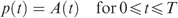
  Note, that solution (A.1) satisfies the optimality conditions (12) (because Y(t)=h(t−T)<c for any t) and (15) (since, with respect to (16), P _min⩽A(t)⩽P _max for 0⩽t⩽T). Moreover, this solution is always feasible if constraint (4) holds, that is, X(T)>0. Substituting p(t)=A(t) from (14) and Y(t)=h(t−T) into from (A.1) we find the inventory condition stated in the proposition.

  Finally, it is readily observed that p(t)=1/2((a−bt)/e+P+h(t−T)) decreases if b/e>h, otherwise it increases.

Proof of Proposition 2

• As shown in Proposition 1, solution (A.1) is feasible and meets the optimality conditions if costs are balanced and X(T)>0. If the costs are not balanced, at least one of the switching points (18) and (19) is feasible, which with respect to (15) implies constant either maximum or minimum price as stated in the proposition. Finally, if both points are feasible for b/e<h, then according to the optimality condition (15), the optimal trajectory consists of three parts:

  

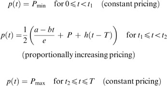
  If b/e>h and the two points are feasible, then the opposite sequence of trajectories is optimal: maximum price, proportionally decreasing price and minimum price.

Proof of Proposition 3

• Consider the following no production solution to (1), (2), (3) and (4) and (10) and (11):

  

  This solution satisfies the optimality conditions (15), P _min⩽A(t)⩽P _max for 0⩽t⩽T and (12), Y(t)<c, 0⩽t⩽T, if r does not exceed the unit production cost, r⩽c which is why r is referred to as reduced production cost. Moreover, this solution is always feasible if X(T)=0, for Y(t)=r+h(t−T).

  Substituting p(t)=A(t) (from (14)) and Y(t)=r+h(t−T) into

  

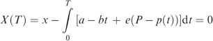
  we find r, as stated in the proposition. The two inventory conditions stated in the proposition are then immediately obtained by requiring 0<r⩽c. Finally, it is easy to observe the same effect of the relationship between b/e and h on the optimal pricing as determined in Proposition 1.

Proof of Proposition 4

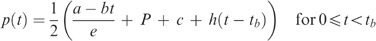
• Consider the following no-production until a breaking point solution to (1), (2), (3) and (4) and (10) and (11), which is followed by exact tracking of the demand:

  

  and

  
  

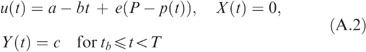
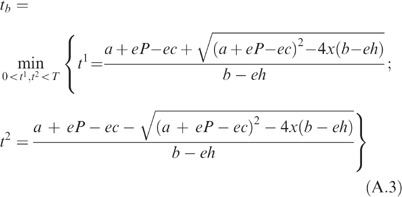
  First note that (A.2) implies that, pricing policy consists of two trajectories separated by a breaking point, t _b :

  

  and

  

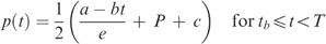
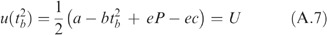
  With respect to Proposition 3, if the initial inventories are not overestimated, that is, x⩽(T/2)(a+eP−ce)−(T ²/4)(b−eh), then the breaking point t _b determined by X(t _b )=0 is feasible. Therefore, using (1), (14) and (A.2) we find

  

  and, thus,

  

  Note, that solution (A.2) meets optimality condition (15) and (12). Moreover, this solution is always feasible if the system has enough capacity to trace the demand exactly, that is,

  

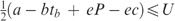
  Taking into account (A.2), condition (A.4) implies

  

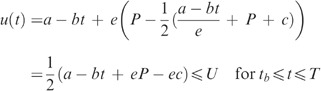
  Since the demand is negatively sloped, the last condition is ensured if it is met at the breaking point, as stated in the proposition.

Proof of Proposition 6

• Consider the following solution to (1), (2), (3) and (4) and (10) and (11)

  

  and

  
  
  

  Taking into account (1) and (14), solution (A.5) implies that

  

  and,

  

  from where the equations for the two breaking points are readily obtained as stated in the proposition.

  Solution (A.5) evidently satisfies the optimality conditions (12) and (15). Moreover, from Proposition 4, it follows that this solution is feasible as well if the capacity constraint derived in Proposition 4 does not hold. Therefore, requiring , as stated in Proposition 6, concludes the proof.

References

Arrow KA, Harris TE and Marschak J (1951). Optimal inventory policy. Econometrica 19: 250–272.
Morse MP and Kimbal GE (1951). Methods of Operations Research. MIT Press: Cambridge, MA.
Khouja M (1999). The single period (news-vendor) inventory problem: a literature review and suggestions for future research. Omega 27: 537–553.
Silver EA, Pyke DF and Peterson R (1998). Inventory Management and Production Planning and Scheduling. Wiley & Sons: New York.
Elmaghraby W and Keskinocak P (2003). Dynamic pricing in the presence of inventory consideration: research overview, current practice, and future directions. Mngt Sci 49: 1287–1309.
Chan L, Simhi-Levi D and Swann J (2002). Dynamic pricing strategies for manufacturing with stochastic demand and discretionary sales. Working paper, Georgia Institute of Technology, Atlanta, GA.
Chen X and Simhi-Levi D (2002). Coordinating inventory control and pricing stratagies with random demand and fixed ordering costs. Working Paper, Massachusetts Institute of Technology, Cambridge, MA.
Federgruen A and Heching A (1999). Combined pricing and inventory control under uncertainty. Opns Res 47: 454–475.
Pekelman D (1974). Simulteneous price-production decisions. Opns Res 22: 788–794.
Feichtinger G and Hartl RF (1985). Optimal pricing and production in an inventory model. Eur J Opl Res 19: 45–86.
Rajan A, Rakesh R and Steinberg R (1992). Dynamic pricing and ordering decisions by a monopolist. Mngt Sci 38: 240–262.
Jorgensen S, Kort PM and Zaccour G (1999). Production, inventory and pricing under cost and demand learning effects. Eur J Opl Res 117(2): 382–395.
Kalish S (1983). Monopolist pricing with dynamic demand and production cost. Marketing Sci 2(2): 135–159.
Paroush J and Spiegel U (1995). Price discrimination with one-way separated markets. Int J Econ Business 2: 441–442.
Maimon O, Khmelnitsky E and Kogan K (1998). Optimal Flow Control in Manufacturing Systems: Production Planning and Scheduling (Applied Optimization, Volume 18). Kluwer: Dordrecht.
Author information
Authors and Affiliations
Corresponding author