Pairwise opposite matrix and its cognitive prioritization operators: comparisons with pairwise reciprocal matrix and analytic prioritization operators

Abstract

The pairwise reciprocal matrix (PRM) of the analytic hierarchy/network process has been investigated by many scholars. However, there are significant queries about the appropriateness of using the PRM to represent the pairwise comparison. This research proposes a pairwise opposite matrix (POM) as the ideal alternative with respect to the human linguistic cognition of the rating scale of the paired comparison. Several cognitive prioritization operators (CPOs) are proposed to derive the individual utility vector (or priority vector) of the POM. Not only are the rigorous mathematical proofs of the new models demonstrated, but solutions of the CPOs are also illustrated by the presentation of graph theory. The comprehensive numerical analyses show how the POM performs better than the PRM. POM and CPOs, which correct the fallacy of the PRM associated with its prioritization operators, should be the ideal solutions for multi-criteria decision-making problems in various fields.

Appendix

A.1. Proofs

Proposition 1 Proof:

• ∑ _i ∑ _j b _ij = ∑ _i ∑ _j>i (b _ij + b _ji ) + 0. I = 0, where I is the identity matrix and b _ij +b _ji =0. □

Proposition 2 Proof:

• The proof is trivial. Let b _ij =v _i −v _j , b _ik =v _i −v _k , b _jk =v _j −v _k , then

  b _ik +b _jk =(v _i −v _k )−(v _j −v _k )=v _i −v _j =b _ij , ∀k∈(1, …, n). □

Proposition 3 Proof:

• For B _j ={b _1j , …, b _nj }^T, then B _j ^T={b _1j , …, b _nj }.

  Since B _i ={b _i1, …, b _in } and B _j ^T={b _1j , …, b _nj }, then B _i +B _j ^T={b _i1+b _1j , …, b _in +b _nj }.

  Case 1: B is perfectly accordant:

  As b _ik +b _kj =b _ij , k∈(1, …, n), then b _ij ∈{b _i1+b _1j , …, b _in +b _nj }.

  Thus B _i +B _j ^T−b _ij =0 × e ⁿ, where n-identity row e ⁿ is the row of n identity elements, for example

  Thus {d _ij }={0}. AI=0.

  Case 2: B is not accordant:

  Let B _i +B _j ^T={b _i1+b _1j , …, b _in +b _nj }={b ₁′, …, b _n ′}, and then

  B _i +B _j ^T−b _ij ={b ₁′, …, b _n ′}−b _ij .

  To normalize the above form, then 1/κ(B _i +B _j ^T−b _ij )=1/κ({b ₁′, …, b _n ′}−b _ij ).

  Next,

  
  

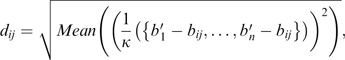
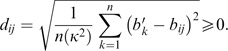
  Thus,

  Under this condition, if AI⩽0.1, B is defined to be unsatisfactory. If AI>0.1, B is defined to be unsatisfactory. □

Proposition 4 Proof:

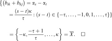
• Let a scale item of the rating scale be the form α _i ∈X̄, and α _i =i′κ/τ, i′ =−τ, …, −1,0,1, …, τ. If b _ik =α _s and b _jk =α _t , then α _s −α _t =(s−t)κ/τ.

  Since s, t∈{−τ, …, −1,0,1, …, τ} and s≠t, then α _s −α _t =(s−t)κ/τ.

  This follows Min({(s−t)})=−2τ and Max({(s−t)})=2τ.

  In other words, (s−t)∈{−2τ, −2τ+1, …, −τ…0,…,τ…,2τ−1,2τ}.

  If (s−t)>τ or (s−t)<τ, then (b _ik −b _jk )=(α _s −α _t )>κ or (b _ik −b _jk )=(α _s −α _t )<κ.

  As Max (X̄)=α _τ =τκ/τ=κ and Min (X̄)=α _−τ =−τκ/τ=−κ, that is X̄=[−κ, …, κ] and (b _ik −b _jk )=(α _s −α _t )>κ or (b _ik −b _jk )=(α _s −α _t )<κ , then an outbound error exists.

  Otherwise, that is−τ⩽(s−t)⩽τ, the POM is within boundary.

  If this happens, then

  

Theorem 1 Proof:

• B≅B̃

  B+V≅B̃+V=n × V, which is written explicitly,

  
  
  

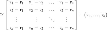
  Thus,

  
  
  

  Thus the solution is found. □

Theorem 2 Proof:

• This theorem can be proved by the Gaussian elimination method in which the augmented matrix [E _i ¦b _i ] is transformed to the reduced row echelon form [I¦ω _i ]. Explicitly,

  
  
  

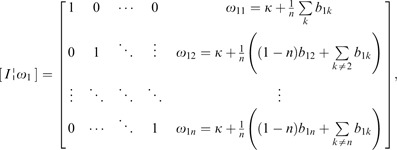
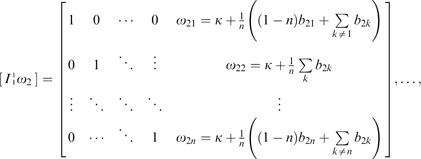
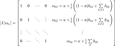
  Thus, the general form is as shown in Equation (16). □

Proposition 5 Proof:

• For an accordant matrix, there should be a solution set in the linear systems set L=(L ₁, …, L _n }, which can be represented by the augmented matrices. The row reduction of L returns a row echelon form. If the row echelon form contains a vector (0 … 0¦c) where c is a constant, this means the matrix has no solution. Otherwise, L has a unique solution.

  It can be proved that when ω _i ≠ω _j , ∀i, j=1, …, n, the row echelon form must contain a vector (0 … 0¦c). This means that L has no unique solution and the matrix is discordant. Otherwise, L has unique solution set and A is the accordant matrix. □

Theorem 3 Proof:

• Let ω _i =(ω _i1, …, ω _in ), i=1, …, n. Then

  
  
  
  
  
  

  which is divided into two cases:

  Case 1:

  As b _ik =−b _ki ,

  

  Case 2:

  

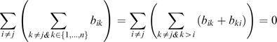
  To combine both cases,

  

Proposition 6 Proof:

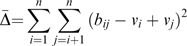
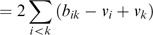
• The objective function minimizes the sum of {Δ _ij ²}, that is Min ∑ _i=1 ⁿ∑ _j=1 ⁿΔ _ij ². This gives ∑ _i=1 ⁿ∑ _j=i+1 ⁿΔ _ij ²=∑ _i=1 ⁿ∑ _j=1 ^jΔ _ij ², that is ∑ _i=1 ⁿ∑ _j=i+1 ⁿ(b _ij −v _i +v _j )²=∑ _i=1 ⁿ∑ _j=1 ^j(b _ij −v _i +v _j )²=Δ̄. Thus, ∑ _i=1 ⁿ∑ _j=i ⁿ(b _ij −v _i +v _j )²=∑ _i=1 ⁿ∑ _j=i+1 ⁿ(b _ij −v _i +v _j )²⁺∑ _i=1 ⁿ∑ _j=1 ^j(b _ij −v _i +v _j )²=2Δ̄. Hence, this proposition holds. □

Theorem 4 Proof:

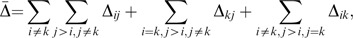
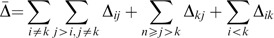
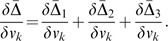
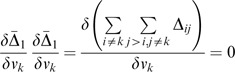
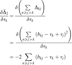
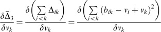
• To have the closed form solution, the partial differentiation of Δ̄ with respective to all v _k ∈V is derived and is of the form:

  

  Then the linear system {L _i } is solved for V. Therefore,

  
  
  

  Let and Thus

  
  

  Case 1:

  

  Case 2:

  

  Case 3:

  
  

  To combine the three cases,

  

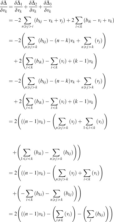
  Since ∂²Δ̄/∂v _k =2(n−1)>0, Δ̄ is convex.

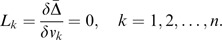
  As L _k =δ²Δ̄/δv _k =0, k=1, 2 ,…, n, there exists a minimal v _k , k=1, 2 ,…, n.

  The values can be solved by a linear system. Thus the augmented matrix [E¦b] is of the form:

  

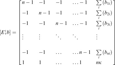
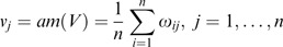
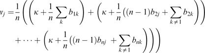
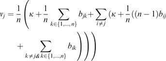
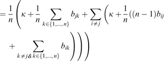
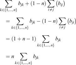
  V is solved by Gaussian elimination of [E¦b], in which the final row is added to other rows. Thus,

  

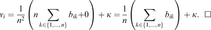
  To divide the above system by n, the reduced row echelon form is

  

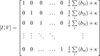
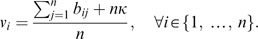
  Interestingly, the result is the same as the row average plus the normal utility. □

Proposition 7 Proof:

• For ∀i∈{1, …, n}, if v _i ⩾0, then (1/n∑ _j=1 ⁿ b _ij ). If (1/n∑ _j=1 ⁿ b _ij ), then Max (ℵ)⩽κ since b _ij ∈ℵ.

References

Barzilai J (1997). Deriving weights from pairwise comparison matrices. J Opl Res Soc 48: 1226–1232.
Belton V and Gear T (1983). On a shortcoming of Saaty's method of analytic hierarchies. Omega 11 (3): 228–230.
Blankmeyer E (1987). Approaches to consistency adjustment. J Optim Theory Appl 54: 479–488.
Bryson N (1995). A goal programming method for generating priority vectors. J Opl Res Soc 46: 641–648.
Budescu DV, Zwick R and Rapoport A (1986). A comparison of the eigenvalue method and the geometric mean procedure for ratio scaling. Appl Psychol Measure 10: 69–78.
Chandran B, Golden B and Wasil E (2005). Linear programming models for estimating weights in analytic hierarchy process. Comput Opns Res 32: 2235–2254.
Chu ATW, Kalaba RE and Spingarn K (1979). A comparison of two methods for determining the weights of belonging to fuzzy sets. J Optim Theory Appl 27: 531–541.
Costa CAB and Vansnick J-C (2008). A critical analysis of the eigenvalue method used to derive priorities in AHP. Eur J Opl Res 187: 1422–2428.
Crawford G and Williams C (1985). A note on the analysis of subjective judgement matrices. J Math Psychol 29: 387–405.
Dyer JS (1990a). Remarks on the analytic hierarchy process. Mngt Sci 36 (3): 249–258.
Dyer JS (1990b). A clarification of ‘Remarks on the analytic hierarchy process’. Mngt Sci 36 (3): 274–275.
Figueira J, Greco S and Ehrgott M (eds). (2005). Multiple Criteria Decision Analysis: State of the Art Surveys. Springer: New York.
Forman EH and Gass SI (2001). The analytic hierarchy process: An exposition. Opns Res 49 (4): 469–486.
Forman EH and Selly MA (2001). Decision by Objectives: How to Convince Others That You Are Right. World Scientific: Singapore.
Golany B and Kress M (1993). A multicriteria evaluation of methods for obtaining weights from ratio-scale matrices. Eur J Opl Res 69: 210–220.
International Society on Multiple Criteria Decision Making (2009). Multiple criteria decision aid bibliography. http://www.lamsade.dauphine.fr/mcda/biblio.
Lin C-C (2006). An enhanced goal programming method for generating priority vectors. J Opl Res Soc 57: 1491–1496.
Mikhailov L (2000). A fuzzy programming method for deriving priorities in the analytic hierarchy. J Opl Res Soc 51 (3): 341–349.
Murphy CK (1993). Limits on the analytic hierarchy process from its consistency index. Eur J Opl Res 65: 138–139.
Perez J (1995). Some comments on Saaty's AHP. Management Science 41: 1091–1095.
Saaty TL (1980). Analytic Hierarchy Process: Planning, Priority, Setting, Resource Allocation. McGraw-Hill: New York.
Saaty TL (1994). Fundamentals of Decision Making. RSW Publications: Pittsburgh.
Saaty TL (2000). Fundamentals of Decision Making and Priority Theory with the Analytic Hierarchy Process. RWS Publications: Pittsburgh.
Saaty TL (2001). Decision Making for Leaders: The Analytic Hierarchy Process for Decisions in Complex World. 3rd edn, RWS Publications: Pittsburgh, (1st edn. in 1982).
Saaty TL (2005). Theory and Applications of the Analytic Network Process: Decision Making with Benefits Opportunities, Costs, and Risks. RWS Publications: Pittsburgh.
Saaty TL (2008). Relative measurement and its generalization in decision making: Why pairwise comparisons are central in mathematics for the measurement of intangible factors—The analytic hierarchy/network process. RACSAM (Rev Roy Spanish Acad Sci, Ser A, Math) 102 (2): 251–318.
Saaty TL and Vargas LG (1984). Comparison of eigenvalue, logarithmic least squares and least squares methods in estimating ratios. Math Modelling 5: 309–324.
Srdjevic B (2005). Combining different prioritization methods in the analytic hierarchy process synthesis. Comput Opns Res 32: 1897–1919.
Thurstone LL (1927). A law of comparative judgment. Psychol Rev 34: 273–286.
Vaidya OS and Kumar S (2006). Analytic hierarchy process: An overview of applications. Eur J Opl Res 169 (1): 1–29.
Wang YM and Elhag TMS (2006). An Approach to avoiding rank reversal in AHP. Decis Supp Syst 42: 1474–1480.
Whitaker R (2007). Criticisms of the analytic hierarchy process: Why they often make no sense. Math Comput Modelling 46: 948–961.
Yuen KKF (2009). Cognitive network process with fuzzy soft computing technique for collective decision aiding. PhD thesis, The Hong Kong Polytechnic University.
Yuen KKF (2010). Analytic hierarchy prioritization process in the AHP application development: A prioritization operator selection approach. Appl Soft Comput 10 (4): 975–989.
Zahedi F (1986). A simulation study of estimation methods in the analytic hierarchy process. Socio Econ Plan Sci 20: 347–354.
Acknowledgements
The research work is essentially derived from the author's PhD thesis, The Hong Kong Polytechnic University. Thanks are also extended to the anonymous referees for their time and effort to improve the work.
Author information
Authors and Affiliations
Corresponding author