
Abstract
This article provides an improvedmodel-independent lower bound of European call options written on defaultable assets. On the basis of static arbitrage arguments, improved lower bounds are established, which also depend on the probability of option-implied default. The results are also extended to dividend-paying stocks. Moreover, our findings imply that it is never optimal to exercise certain American call options. Finally, we discuss the implications of our results for constructing an arbitrage-free volatility surface and extracting risk-neutral densities from option prices.
INTRODUCTION
One of the classic results of financial economics is that the model-independent lower bound of European call option is given by either zero or the underlying price minus the present value of the exercise price (Merton, 1973). This result can be easily verified by constructing a portfolio with 0 initial value, which yields a profit with positive probability without taking any risk.
Since Merton’s seminal paper, the bounds on option prices have been tightened using a variety of approaches (see Handley, 2005, for a comprehensive review). However, the probability of default of the underlying is rarely addressed in this context. Although some recent work by Klein and Yang (2013) explores the early exercise of American options in the presence of counterparty credit risk, their results are too general to be applicable to our case.
In this article, we present an improved lower bound of European call options written on defaultable assets when the option-implied probability of default is observable in the market. Moreover, we demonstrate that exercising American calls early is not an optimal strategy in certain cases. Finally, we discuss the implications of our results for some financial engineering applications.
ASSUMPTIONS AND NOTATION
Following Merton (1973), we make the following assumptions: (i) capital markets are perfect; (ii) there is no arbitrage; (iii) investors have positive marginal utility of wealth; and (iv) current and future interest rates are strictly positive. In addition, we assume that if a company defaults, its stock price is worthless. On the basis of these conditions, consider a stock that has a current price of S0 with a positive risk-neutral default probability of PD before some time T. Then, the risk-neutral probability of the asset not defaulting before time T can be expressed as:

where S T is the price of the asset at time T, and P(S T >0) is the risk-neutral probability of S T >0. Moreover, let C(K, T) be the current price of a European call option on the stock with strike K, maturity T. It can be shown (see, for example, Orosi, 2011) that

where P(S T >K) is the risk-neutral probability of S T being greater than K and B(K, T) is a European-style binary option with strike price K and maturity T. Substituting K=0 into the above yields

Note that the price of the digital contract, D(T), that pays a unit currency if default happens before time T at time T and 0 otherwise is given by

and that this contract can be replicated by call options and cash as follows. From equations (1) and (2):

GENERAL RESULTS
Improved lower bound
We start our analysis by first considering a non-dividend-paying stock. We will, in a later section, extend our result to dividend-paying assets and examine the implications.
Proposition 1
-
The lower bound of a European call option written on a defaultable asset is
Proof
-
Assume otherwise and form the following 0 value portfolio at time 0:


where K⋅e−rT and B represent the amounts invested in bonds. In the case of default, the value of the portfolio at the time of expiry is given by:

because the stock and call option become worthless and the payoff of D(T)=1. If the asset does not default before expiry and the option does not finish in the money (or S T <K equivalently), then the value of the portfolio at the time of expiry is given by

because the call option and D(T) become worthless. Finally, if the asset does not default before expiry and the option finishes in the money (or S T >K equivalently), then the value of the portfolio at the time of expiry is given by

Therefore, if equation (4) does not hold, a portfolio can be constructed that yields static arbitrage violation. □
Moreover, it should be noted that equation (4) is higher than Merton’s lower bound of S0−K⋅e−rT as long as PD>0.
Known dividend payments
Consider a stock written on a defaultable asset that is certain to pay a single dividend of D at the ex-dividend date, t where 0<t<T.
Proposition 2
-
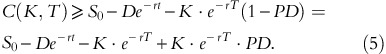
The lower bound of a European call option written on a defaultable asset is

Proof
-
Assume otherwise and form the following 0 value portfolio at time 0:

where K⋅e−rT, De−rt and B represent the amounts invested in bonds. If the asset does not default before expiry, the value of this portfolio at time T is the same as in the case of the non-dividend-paying stock.
If the stock defaults after dividend payment, the value of the portfolio at the time of expiry is given by

If the stock defaults before dividend payment, the value of the portfolio is larger than BerT because dividend will not be paid.
Therefore, equation (5) must hold to prevent static arbitrage opportunities. □
Note that the results can be easily generalized to multiple known dividends. In this case, the following must hold:

where D is the present value of future dividends expected to be paid before T.
Proposition 3
-
Early exercise of an American call option is not optimal, if the following relationship holds:


Proof
-
On the basis of equation (6), an American call option must be worth at least

because the value of an American option is always greater than or equal to the value of a corresponding European option. Hence, assuming equation (7) holds, the value of an American call option at some time T* must be worth at least

Since the above value is strictly greater than the value of early exercise,  the claim is proven. □
DISCUSSION AND FUTURE RESEARCH
A robust method for constructing a continuous call option surface from a given set of option prices is of great interest for academicians and practitioners. For example, Figlewski (2009) uses risk-neutral density (RND) to obtain information about investors’ risk preferences and expectations. Some important examples of financial engineering applications are the pricing illiquid exotic derivatives with arbitrary payoffs, copula-based pricing of multi-asset products, and reconstructing a local volatility surface. For example, Monteiro et al (2011) show that implied RND can be used to accurately price European-style binary options, Cherubini and Luciano (2002) use implied RND to price bivariate equity options and Fengler (2009) uses an interpolant to recover the local volatility surface.
Figlewski (2009) points out that interpolation is typically performed in the implied volatility space, which involves fitting a spline or a low-order polynomial to the available data. Although such techniques have excellent empirical performance (see Orosi, 2012), Benaim et al (2008) assert that implied volatility-based models should not be used when there is a positive probability of default. Therefore, in certain cases, existing interpolation methods should be abandoned or modified to include the results from this study. For example, Benaim et al (2008) and Orosi (2014) both introduce techniques that do not violate the improved bounds.
Another potential area of research may examine whether lower bound violations occur in empirical data. For an example of such a study, see Dixit et al (2009).
CONCLUSION
In this article, we derive lower bounds for European options written on defaultable assets. We demonstrate that these bounds are tighter than the existing lower bounds and discuss the implications of our findings.
References
Benaim, S., Dodgson, M. and Kainth, D. (2008) An arbitrage-free method for smile extrapolation, Working Paper, QuaRC, Royal Bank of Scotland.
Cherubini, U. and Luciano, E. (2002) Bivariate option pricing with copulas. Applied Mathematical Finance 9 (2): 69–85.
Dixit, A., Yadav, S.S. and Jain, P.K. (2009) Violation of lower boundary condition and market efficiency: An investigation into the Indian options market. Journal of Derivatives and Hedge Funds 15 (1): 3–14.
Fengler, M.R. (2009) Arbitrage-free smoothing of the implied volatility surface. Quantitative Finance 9 (4): 417–428.
Figlewski, S. (2009) Estimating the Implied Risk-Neutral Density for the US Market Portfolio, Volatility and Time Series Econometrics: Essays in Honor of Robert F. Engle. Oxford, UK: Oxford University Press.
Handley, J. (2005) On the upper bound of a call option. Review of Derivatives Research 8 (2): 85–95.
Klein, P. and Yang, J. (2013) Counterparty credit risk and American options. Journal of Derivatives 20 (4): 7–21.
Merton, R.C. (1973) Theory of rational option pricing. Bell Journal of Economics and Management Science 4 (1): 141–183.
Monteiro, A.M., Tütüncü, R.H. and Vicente, L.N. (2011) Estimation of risk neutral density surfaces. Computational Management Science 8 (4): 387–414.
Orosi, G. (2011) A multi-parameter extension of Figlewski’s option-pricing formula. Journal of Derivatives 19 (1): 72–82.
Orosi, G. (2012) Empirical performance of a spline-based implied volatility surface. Journal of Derivatives & Hedge Funds 18 (4): 361–376.
Orosi, G. (2014) Estimating option implied risk neutral densities: A novel parametric approach. Working Paper. Available at SSRN: http://ssrn.com/abstract=2260360.
