The Effect of Pre-commitment and Past-Experience on Insurance Choices: An Experimental Study

Abstract

This paper reports results from an experimental study that investigates insurance behaviors in low-probability, high-loss risk situations. The study reveals that insurance behaviors may depend on the length of the commitment period of insurance policies, namely the period during which individuals commit themselves to maintain the same insurance decision. The results of this study also seem to support the predictions of the Dual Theory concerning the demand for co-insurance policies, that is to say the preference of individuals for extreme (null or full) levels of insurance coverage. This study also suggests that prior risk occurrences influence subsequent insurance choices. The paper provides a new possible explanation about the puzzling fact that people usually fail to obtain insurance against disaster-type risks such as natural disasters, even when premiums are close to actuarially fair levels.

Introduction

The issue of the weak level of insurance demand against low-probability risks

The study of individual insurance behaviors against disaster-type risks, namely high-loss events with a low probability of occurrence, has both theoretical and practical relevance. From a theoretical perspective, the aim is to understand the reasons for which there is a so large a gap between real insurance behaviors and the predictions from the expected utility theory. One of the most striking empirical facts studied in particular by Kunreuther (1996) and Kunreuther and Roth (1998) is that people usually fail to obtain insurance against low-probability high-consequence risks such as natural disasters, even when the terms are quite favorable (e.g. subsidized policies). Several field studies (Coursey et al., 1987) and experimental studies (McClelland et al. (1993)) also reveal a dichotomy in risk perceptions and insurance behaviors from subjects confronted with low-probability risks. People appear either to dismiss the risk and pay nothing for insurance, or to worry too much about the risk and pay premiums that are considerably in excess of the expected loss. The latest empirical evidence is close to the theoretical predictions of the Dual Theory from Yaari (1987), but it remains unexplained within the expected utility framework. From a practical perspective, the aim is to find solutions in order to raise the level of insurance demand in situations where welfare analysis shows that it will be favorable for the global community in the case of natural disasters, for instance.

The motivation of this study: test the role of commitment period on insurance coverage

The main goal of this paper is to test the role of commitment period on insurance coverage, and to provide a new possible explanation for the weak level of insurance coverage commonly observed for low-probability risk. By definition, low-probability risks occurred infrequently on average, and the period of time between two risk occurrences can be very long. Thus, low-probability risks can be considered as a long-term phenomenon because its consequences should be weighted up in the long run. However, risk insurance policies are usually written for a short period of time, namely 1 year. The discrepancy between this short commitment period and the long interval between two risk occurrences may penalize the attractiveness of insurance, as we will see in this study.

The paper is structured as follows. The next section presents the theoretical background and the hypotheses tested in this experimental study. The subsequent section describes the experimental design and procedures. The penultimate section presents the main results of the study. Finally, the last section discusses the theoretical implications of these results and their practical relevance for insurance markets against disaster-type risks.

Theoretical background

Related literature about the influence of the commitment period upon insurance choices

There is evidence, both empirical and theoretical, that people usually have a tendency to evaluate outcomes frequently when they are confronted with sequences of investment opportunities. This short time horizon for evaluation seems to influence the willingness to take risks. For instance, Benartzi and Thaler (1995) propose an explanation for the equity premium puzzle by showing that investors could be reluctant to take risk if they evaluate frequently their portfolio. The link between time horizon and risk taking is based on the combination of two behavioral concepts: loss aversion (Tversky and Kahneman, 1992), which refers to the tendency of individuals to weigh losses more heavily than gains, and mental accounting (Thaler, 1999), which refers to the set of cognitive operations used by individuals to organize, evaluate and keep track of financial activities. The influence of the length of the evaluative period on risk taking is also supported by two later experimental studies from Gneezy and Potters (1997) and Thaler et al. (1997).

Langer and Weber (2001) further refine the relationship between the evaluation period and the willingness to take risk by adding two more behavioral concepts to loss aversion and mental accounting, namely diminishing sensitivity that refers to the tendency of individuals to be risk averse in the gain domain and risk seeking in the loss domain, and probability transformation that refers to the tendency of individuals to weigh probabilities in a non-linear way. The combination of all these behavioral concepts within the same framework is called “Myopic Prospect Theory” (MPT). Diminishing sensitivity and loss aversion can be captured by the following value function proposed by Tversky and Kahneman (1992), where λ represents loss aversion and δ represents diminishing sensitivity.

Langer and Weber (2003) show subsequently that the effect of changes in the length of the commitment period upon the willingness to invest in risky assets depends on the risk profile of the investment options. In particular, the extension of the commitment period seems to decrease the willingness to invest in risky assets for investment opportunities with a low probability of relatively high losses. This phenomenon is explained by the MPT.

Applied to the domain of insurance decisions, this result could explain why people do not insure against catastrophic risks such as natural disasters. The MPT hypothesis predicts indeed that the willingness to take risk in these situations will be greater if individuals have a short evaluation period. When individuals have a short-term horizon, the advantages of staying uninsured (premium savings) weigh more heavily than the disadvantages (potential uninsured losses). Conversely, staying uninsured is accompanied by more disadvantages than advantages when people have a longer time horizon. In the long run, the probability to experience losses at least one time increases, so that loss aversion raises the disutility of expected losses. At the same time, diminishing sensitivity reduces the attractiveness of additional premium savings.

To illustrate this point, let us consider a simple example. Suppose an individual faces the risk of a $100 loss with a periodic probability of P=0.05. This individual has the choice between being uninsured or staying fully insured upon payment of a $6 premium. If he decides to forgo his insurance and nothing happens, he can expect to save the $6 premium, but he can also lose $100 if something finally occurs. Suppose that this individual evaluates the costs and benefits of such a decision through a utility function U(X) such as the one described above with λ=2.25 and δ=0.88 (we are using here the parameter estimates from Tversky and Kahneman, 1992). Then, the expected prospect utility of not buying insurance is positive if the individual has a time horizon –bounded to one period (E(PT)=0.95.U(+6)+0.05.U(−100)>0), but it is negative if the individual has a time horizon widened to the next two periods: (E(PT)=0.95²U(+12)+0.095U(6−100)+0.05²U(−200)<0). Hence, the individual with a short evaluation period would prefer to forsake his insurance whereas the individual with a long evaluation period would prefer to stay insured. Thus, this experimental study is firstly designed to test the following conjecture:

Forward-looking conjecture

• The level of insurance coverage depends on the length of the commitment period, namely the period during which individuals cannot change their initial insurance choice. In particular, we expect to find that the extension of the commitment period tends to increase the level of insurance coverage.

Related literature about the influence of prior experience towards risk upon insurance choices

There are numerous empirical studies that point out a relationship between insurance behaviors and individual prior experience related to risk. For instance, an empirical analysis conducted by Browne and Hoyt (2000) indicates that flood insurance purchases at the state level correlated highly with the level of flood losses in the state during the prior year, for the period from 1983 to 1993, in the United States. Figure 1 gives a representative example of this phenomenon. It displays the number of flood insurance policies in California from 1996 to 2006. The number of insurance policies increases dramatically in 1998 just after major floods in this state. Afterwards, the number of policies decreases on a regular basis because of the absence of major floods.

Figure 1

Flood insurance policies in California.

Another striking example is provided by Kunreuther (1996), who studied the insurance behaviors of California homeowners during the 1989 Loma Prieta earthquake. In 1989 (before the earthquake), about 34 percent of uninsured homeowners thought that earthquake insurance was unnecessary. By 1990, only about 5 percent thought the same. Moreover, 11 percent of the uninsured households decided to purchase coverage between 1989 and 1990. Kunreuther (1996) also reveals that those who do purchase insurance are likely to cancel policies if they have not made a claim after a few years. For instance, approximately one in five policyholders under the National Flood Insurance Program cancels his coverage each year. In the same way, less than 14 percent of California homeowners have earthquake insurance in 2006, down from 34 percent in 1995 just after the last major earthquake occurred.

From a more theoretical point of view, Tversky and Kahneman (1973a, 1973b) put forward two main heuristics that can explain the influence of prior experience upon risky choices, without income effects. A heuristic is a strategy that reduces the complex tasks of assessing probabilities and predicting values to simpler judgmental operations. The first heuristic is the Availability Bias, according to which people assess the probability of an event by the ease with which occurrences can be brought to mind. A type of event whose occurrences are easily retrieved will appear more numerous and more likely. If an event L is dramatic or recent, it will be more memorable and easier to recall. As a result, it will be considered as more likely. Such reasoning does not take into account the fact that events cannot be predicted. According to the availability heuristic, individuals without prior experience with any loss should dismiss this risk and stay uninsured, whereas those who recently suffered a loss should exaggerate the risk and get fully insured. The second heuristic is the well-known Gambler's Fallacy, according to which the likelihood of an event with a fixed probability increases or decreases depending upon recent occurrences. Thus, individuals who have not been hit by a loss for a long time should increase their level of insurance because they do not want to “push their luck.” Conversely, those recently hit should cancel their insurance policy because they might believe that the chance of loss could not happen twice in a row. It is important to stress that these two heuristics predict exactly opposite results about the relationship between insurance behaviors and prior experience towards risk. Consequently, this experimental study is also designed to test the following conjecture:

Backward-looking conjecture

• The level of insurance coverage depends (positively or negatively) on the individual past experience related to risk.

The experimental design

Description of the design

The effectiveness of an experimental design depends on its capacity to reveal a subject's true preferences without distorting them. In particular, Cubitt et al. (2001) argue that a design must be structured in order to minimize all possible kinds of subject errors (such as misunderstanding experimental procedures, invalid logical inferences, disequilibrium beliefs and false expectations about affect). This is the reason why we have chosen to build an individual choice design rather than a marked-based design, and to use a polytomous choice elicitation mechanism rather than open-ended questions. Transparency and simplicity were two leading criteria used when building the design.

A critical feature: two different treatments called S and L respectively.

Characteristics that both treatments have in common

In each treatment, subjects are confronted with a sequence of 12 identical and independent periods of time. At the beginning of each period, subjects are given 100 euros. They have a low probability P=0.04 of losing completely this initial amount during the period. However, subjects have the possibility of purchasing insurance in order to protect themselves against the risk of loss. Thus, they have to decide which part α (from 0 to 1) of their initial amount they want to insure. The loss probability is clearly specified and common knowledge for all subjects. The insurance premium hypothetically paid is deducted from the initial endowment and subjects are price-takers. This insurance premium is proportional to the rate of insurance coverage. When considering wealth variations from the initial endowment, subjects face at every period a lottery of the general formillustrationwhere p is the loss probability, Π the full-insurance premium, α the coverage rate and L the potential loss. With numerical values used in the experimental design, the lottery becomesillustration

We notice that insurance premiums are loaded at a 50 percent rate for each policy. It is important to stress that subjects could not insure any capital accumulated in a previous period in order to avoid income effects. Hence, the maximum insured endowment is always the same in each period, independent of the outcome of the previous period. It is also important to point out that periodic risks are completely independent between the different periods. Namely, the risk occurrence in T does not depend on the risk occurrence in T−1. As a result, we are able to use the so-called random problem selection mechanism (RPSM) as an incentive mechanism. This mechanism, widespread in experimental economics, operates as follows. After all 12 periods have been recorded, one and only one of the periods is selected at random. Then, the subject's entire payment for taking part in the experiment depends on his final payment in that one period. The final payment of a subject at period T is determined by the following simple formula:

The aim of RPSM is to encourage subjects to treat each problem as if it were the only one that they were facing. It avoids the problem of reference-point and also wealth effects that would be created if subjects were paid according to their performance on each of a number of tasks. Of course, such an incentive mechanism is not perfect and there are some possible criticisms of it (see Harrison (1994) or Holt (1986), which present bias that might affect RPSM). At the same time, Camerer and Hogarth (1999) show that the effect of incentives on experiments is often mixed and complicated. In spite of these reservations, the RPSM appears to be the most satisfactory mechanism for our design. We have not found a better alternative. At each period, subjects have to choose among five different options, which are summed up in Table 1. The final column reports wealth variations from the initial endowment, depending on the state of nature.

Table 1 Description of the five available options for subjects

At the end of the experiment, a debriefing questionnaire is provided in order to collect information about the “rules of thumb” used by subjects in their decision process. The aim of this questionnaire is also to evaluate subjects’ risk perception by asking them about their subjective probabilities. The answers collected are purely hypothetical in nature and are checked with prior insurance decisions that are behavioral data. Thus, the aim of the debriefing is to enhance our understanding of behavioral decisions.

Differences between treatments S and L

The duration of the commitment period is different between the two treatments. In treatment S (short commitment period), subjects commit themselves in an insurance choice for only one single period. In this case, subjects are encouraged to adopt a narrow framing of the decision problem. At the beginning of the first period, they have to choose how much of their initial endowment to insure. Then, they are informed about the risk realization at the end of this first period. As a result, subjects begin the second period knowing the consequences or results of the risk simulation during the first period. During the second period, subjects choose once again the part of their new initial endowment that they want to insure, and so on. The risk simulation in treatment S operates as follows. At the beginning of the experiment, each subject receives a private letter of the alphabet between A and Y (thus, there are 25 possibilities). Each subject does not know the private letter assigned to the other subjects. At each period, the experimenter uses an urn containing 25 different letters also between A and Y. After the subjects have recorded their insurance decision for the current period, the experimenter shakes the urn and randomly takes one letter out of the urn. If a subject's private letter matches the letter taken from the urn, the subject is hurt by the risk and he loses the uninsured part of his endowment. If the letter does not match, the subject sustains no loss. Since there are 25 different letters in the urn, the probability of being hurt by the risk is equal to 1/25=0.04 whereas the probability of sustaining no loss is equal to 24/25=0.96. It is important to note that the letter drawn is always put back into the urn after each drawing. Hence, the probability of loss remains constant for every subject across periods.

In treatment L (long commitment period), subjects commit themselves to an insurance choice for four periods in a row. Hence, they are encouraged to adopt a longer evaluation period. At the beginning of the first period, subjects have to decide how much of their periodic endowment of 100 euros to insure from period no. 1 to period no. 4. Subjects are informed about risk realization only at the end of the fourth period. At the beginning of the fifth period, they choose again for periods 5, 6, 7, 8 and so on. In this treatment, the risk simulation operates as follows. At the end of the fourth period, the experimenter executes four draws in a row from the urn always putting the letter drawn back into the urn between each drawing. Thus, subjects know simultaneously about the risk occurrence in the first block of four periods. After each period or after each block of four periods as in treatment L, subjects calculate and record their final payment on a registration form. The experimenter checks these calculations to make sure that the subjects understood the procedure.

Procedure and implementation

Sixty-four subjects were recruited from the university student community of Le Mans in France. They were all undergraduates and not necessary students in economics. Most of these subjects knew very little about Decision Theory and were not very familiar with concepts such as “probability” or “expected value.” It was the first time that they took part in an experimental economics study. We assume that such “lay” subjects may behave in a more sincere and intuitive way compared to subjects who are used to doing experiments and may be exposed to the panel effect bias. We carried out eight experiment sessions, four for each of the two treatments S and L. About eight different subjects took part in each session, which lasted approximately 1 hour (nearly half the time was spent reading the instructions to subjects, and the rest of time for implementing the experiment itself). The experiment was administered using pen and paper, and held in a classroom with subjects seated far apart. Subjects were not allowed to communicate with each other. At the beginning of the session, instructions were distributed and read aloud and these instructions are given in the Appendix. After that, subjects could look at the instructions for a few additional minutes and privately ask questions. Then, subjects were asked to record their first insurance choice. They then recorded their choice on a paper form and handed it in. The fact that the risk simulation was done “by hand” guaranteed its transparency and should have convinced the subjects that manipulation was impossible (unlike with computerized simulation).

The debriefing questionnaire was filled out after the sequence of behavioral choices, but before subjects learned about their remuneration for taking part in the experiment. At the end of the experiment, subjects received performance-based financial incentives. They could earn up to 100 euros. Financial incentives were based on the RPSM. For each subject, only one period among the 12 was randomly selected. Then, only one subject per group of eight was randomly selected. This subject received the payment for the period that was selected for him. Thus, he could earn up to 100 euros. All of these random selections were carried out by throwing dice.

Experimental results

Commitment period and level of coverage

Observation no. 1

• The length of the commitment period increases the level of insurance coverage.

Table 2 compares the average percentage of the periodic endowment that is fully insured for the two treatments S and L. This average percentage is called the “coverage rate.” In order to make comparisons between treatments easier to understand, this average coverage rate is calculated in blocks of four periods. It is important to stress that both treatments are exactly the same, except for the duration of the commitment period that is longer in treatment L (four rounds in a row) and shorter in treatment S (one single round).

Table 2 Level of insurance coverage among treatments

These results indicate quite a significant treatment effect. It seems that the experimental design is effective in changing subjects’ attitude towards risk. In each period indeed, coverage rates are higher for treatment L than for treatment S. The significance of the difference is determined by a Mann–Whitney test (i.e. a non-parametric test of the null hypothesis that the distribution of an ordinal scale response variable is the same in two independently sampled populations). The critical values show that the differences in average coverage rates are rather significant. The final column in Table 2 reports z-values, which are a transformation of the Mann–Whitney U-value corrected for the presence of ties. The corresponding one-tailed significance levels are also reported. We report one-tailed significance levels because the null hypothesis (E.U theory) predicts no systematic differences, whereas the alternative hypothesis (MPT) predicts that insurance coverage in treatment L will be higher. These results support the prediction of MPT, according to which a longer evaluation period makes an insurance policy look more attractive. It is worth noticing that such differences in behaviors between the two treatments cannot be explained within an expected utility framework, in particular because of the procedural invariance hypothesis. It is also important to stress that the risk simulations were not significantly different among treatments according to the Kolmogorov–Smirnov test (P<0.001). Thus, the observed differences in behaviors cannot be explained by discrepancy among treatments in the simulation of the risk of loss (Figure 2).

Figure 2

Average coverage rate across periods.

Observed data and the Dual Theory of choice

Observation no. 2

• There is a pronounced bi-modality of the distribution of choices among the different insurance options. Null and Full insurance are the most frequently chosen policies. Such a result may be explained within a Dual Theory framework.

  Table 2 reveals that standard deviations are very important in both treatments. As Figure 3 shows, this is due to bi-modality in the distribution of subjects’ choices. Most subjects either do not want to pay anything for insurance or are willing to pay for a full insurance policy with a very high premium (positively loaded at 50 percent).

  Figure 3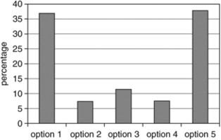

  

  Frequency distribution of all choices (all treatments). Recalling: option 1=no insurance; options from 2 to 4=partial insurance; option 5=full insurance.

  The bimodal results are consistent with the findings of McClelland et al. (1993) and Schade et al. (2004). Moreover, these results are obtained with a different elicitation mechanism. The two modes suggest that two different processes may be operating. Subjects who stay uninsured may believe that the risk is too small to be worth paying an insurance premium (it is the so-called “can’t-happen-to-me” syndrome). On the other hand, subjects who choose full insurance coverage are showing a heightened sensitivity to the risk and are highly risk averse (more risk averse anyway than the EU theory can predict). As a result, some subjects seem to believe the risk to be very significant whereas others judge the risk to be negligible. Many field studies such as Smith and Desvouges (1987) also support the pattern of bi-modality concerning the risk perception of environmental hazards (e.g. hazardous waste sites, radon exposure).

  As the experimental design leads subjects to choose between co-insurance policies, we can notice that the descriptive power of the Dual Theory (Yaari, 1987) is greater than the descriptive power of the EU Theory. Observation no. 2 reveals clearly the significant tendency of subjects to choose extreme insurance policies. As for the Dual Theory framework, Doherty and Eeckhoudt (1995) show that only full or null insurance is optimal for a risk-averse decision-maker insured when premiums are positively loaded. It is never optimal in this case to become partially insured when premiums are positively loaded. Conversely, only partial and null insurance can be explained within the EU theoretical framework. In such a case, it is effectively never optimal for a risk-averse decision-maker to get fully insured because insurance premiums are positively and even heavily loaded (50 percent loading). Figure 4 allows us to compare the descriptive power of Dual Theory vs. EU Theory across periods. This figure displays the significant superiority of Dual Theory in describing the subjects’ behaviors.

  Figure 4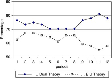

  

  The coherence with Dual Theory and Prospect Theory.

  It is important to stress that Dual Theory has a higher descriptive power in each treatment S and L. In all, 79.8 percent of the observations in treatment S and 68.8 percent of the observations in treatment L are consistent with Dual Theory, but, on the other hand, only 68.4 percent of the observations in treatment S and 55.9 percent of the observations in treatment L are consistent with EU Theory.

  McClelland et al. (1993) proposed that future research should try to determine the factors that predispose individuals to be in the upper mode or in the lower mode, and especially the factors that cause an individual to switch from one mode to another. This point is addressed in observation no. 3.

Observation no. 3

• The dominant mode is different among treatments: Whereas “full insurance” is the dominant mode in treatment L, “null insurance” is the dominant mode of treatment S.

  Aggregate data such as the frequency distribution depicted in Figure 3 hide important differences between the two treatments. Figures 5a and b present separate data for both treatments S and L. These figures display a clear treatment effect upon bi-modality.

  Figure 5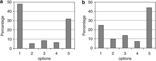

  

  Frequency distribution in (a) treatment S and (b) treatment L.

  It appears that the extension of the commitment period helps change the dominant mode of the frequency distribution of choices. A high proportion of subjects stay uninsured in treatment S, but a high proportion of subjects choose a full insurance policy in treatment L. It is important to stress that this bimodality is due to significant differences among individuals than due to the instability of subjects’ behaviors. The proportion of subjects always insured at least partially is almost two times higher in treatment L than in treatment S. Approximately 61.3 percent of subjects always get insured at least partially in treatment L, compared with only 33.3 percent in treatment S. These subjects are consistently risk-averse towards the low-probability risk. On the other hand, the proportion of subjects almost never insured (less than two periods out of the 12) is two times lower in treatment L than in treatment S. Only 12.9 percent of subjects almost never get insured in treatment L, compared with 27.4 percent in treatment S.

  The answers made by subjects in the debriefing questionnaire bring an additional information about their behaviors. Some subjects initially dismiss the risk but over periods, as the loss does not occur, they judge that the risk is becoming more likely. Other subjects raise significantly their level of insurance just after a risk occurrence or/and withdrawing insurance policy after several periods without risk occurrence. Only 3.1 percent of the subjects seem to adopt an inconsistent and inexplicable behavior with fluctuations. As we used polytomous responses rather than open-ended responses as an elicitation mechanism, it may have reduced the possibility to observe availability and gambler's fallacy heuristics. Furthermore, the bimodality in behaviors may also have reduced this possibility. For instance, a subject who is already fully insured cannot increase his coverage rate still further. In the same way, a subject who is already uninsured cannot reduce his coverage rate still further.

The logistic analysis

Observation no. 4

• Both prior occurrences of risk and commitment period have a significant influence on individual insurance choices.

  The influence of prior risk occurrences and commitment period on individual insurance choices is examined through a multinomial logit model, which is a form of statistical modeling often appropriate for categorical outcome variables. We assume that there is some underlying probability of buying an insurance policy that is function of prior risk occurrences and commitment period.

  

  The subject's insurance choice Y is described through a polytomous response variable that can take five different values coded from 1 to 5 (as many as there are insurance options). The aim of the logit model is to carry out a general regression taking into account all data from both treatments S and L. The concern is that subjects did not face exactly the same decision problems in the two treatments. In fact, the commitment period is not the same. However, we can consider that the decision is quite the same for each block of four periods, which is actually what is implied by the commitment period. Thus, the data of both treatments S and L can be merged per each block of four periods. The three explanatory variables are the following: X₁ can take two values: −1 or 1, and refers to recent risk occurrences (i.e. whether the subject is hurt or remains unhurt by the risk during the last block of four periods). X₂ can also take two values: −1 or 1, and refers to remote risk occurrences (i.e. whether the subject was hurt or was unhurt by the risk before the last block of four periods). Finally, X₃ can also take two value: −1 or 1, and refers to the length of the commitment period (i.e. whether the subject belongs to treatment L or S).

  It is obvious that the explanatory variables X₁ and X₂ are completely independent since the risk simulation because the letters are put back in the urn. As the Kolmogorov–Smirnov test reveals no significant differences in the risk simulation among treatments, we also find no significant relationship between X₃ and the other two explanatory variables. We performed the logistic analysis by using the logistic procedure in the SAS system, which is based on maximum likelihood estimates. The resulting parameters, chi-square and standard errors are reported in Table 3, where the parameters represent the differential changes in the log odds due to the change of the explanatory variables.

  Table 3 Analysis of maximum likelihood estimates

  We find that the tests for assessing model fit through explanatory capability are supportive of the model. The likelihood ratio test has a value of 55.402 and the score test has a value of 46.528 with four degrees of freedom. Hence, the global null hypothesis is excluded and the conclusion is that the model is globally significant. Rather than relying on maximum likelihood estimates to interpret the logistic regression, we prefer to use odds ratio estimates that are more easily interpretable. Table 4 presents the odds ratio estimates for the three explanatory variables.

  Table 4 Odds ratio estimates of choosing a lower insurance coverage

  Let us consider the influence of faraway risk occurrences (i.e. risk occurrences before the last block of four periods). Odds ratio of 3.626 tells us that the predicted odds of choosing a lower insurance rate if subject was unhurt before the last block of four periods is about 3.62 times the odds for a subject that has been hurt before the last block of four periods. In other words, the odds of choosing a lower insurance level for subjects unhurt before the last block of four periods is about 262 percent greater than the odds for subjects hurt by the risk before the last block of four periods. This partial effect is rather significant since the Wald test shows that the odds ratio is significantly different from 1.

  The length of commitment period also appears to have a significant effect upon insurance choices. Subjects with a short commitment period have about four times the odds of choosing a lower level of insurance, compared to those with a long commitment period. On the other hand, the factor (recent risk occurrences) appears to be much less significant as we cannot reject the hypothesis that the first odds ratio in Table 4 is significantly different from 1.

  One interesting advantage of the logit analysis is that we can deduce from the odds estimates the predicted probabilities that a subject will choose a particular insurance option, depending on the past risk occurrences and the length of the commitment period. Table 5 displays those predicted probabilities. “Hurt recently” means that the subject was hurt during the last block of four periods, and “hurt not recently” means that the subject was hurt before the last block of four periods. It is important to stress that those probabilities have to be interpreted very cautiously because all parameters are not significant as seen in Table 3.

  Table 5 Predicted probabilities conditional to subject profile

  The probability to stay uninsured P(Y=1) is the greatest for subjects always unhurt (recently and not recently) and with a short commitment period. Subjects hurt both recently and not recently, and with a long commitment period have the greatest probability to choose full insurance P(Y=5). Such a result seems to support our previous observations. The lack of insurance demand may be due to the lack of prior experience towards the risk of loss and/or too short a commitment period.

Discussion and conclusion

The results from this experimental study suggest that insurance behaviors in the face of low-probability risks may depend on the duration of the commitment period as well as prior risk occurrences and subjective risk perception. Of course, this experiment is highly stylized and does not reflect exactly real-life situations. Indeed, subjects face one single binary risk with an unambiguous probability of occurrence, whereas real-life homeowners confronted with natural hazards may deal with uncertainty and background risk. Moreover, the financial stakes for the subjects may be low compared with those associated with natural disasters in real life. Thus, these features are a cause for caution in the extrapolation of the results. Nevertheless, this experimental study provides some results that may have both theoretical interest and empirical relevance. Many empirical facts indicate that there is a limited demand for disaster insurance. The underestimation of the risk appears to be one of the main factors that leads many individuals to stay uninsured. Our experimental study provides new elements that help to understand the reasons of this underestimation of the danger. The underlying ideas are illustrated in Figure 6.

Figure 6

Time horizon and risk perception.

Let us define short-term awareness as the tendency of an individual to have both limited memory (i.e. amnesia) and short-term horizon of evaluation (i.e. myopia). On the one hand, an individual with limited memory may not remember that risks have previously happened in the past. According to the availability bias heuristic, such a situation could lead to risk underestimation. On the other hand, an individual with short-term horizon may not anticipate that risk can occur again in the future. According to MPT, such a situation could also lead to the underestimation of the danger. Since the frequency of major natural hazards is very low (centennial and even more), it may be difficult for an individual to remember about past occurrences of the risk (especially if they occurred in previous generations), as well as to imagine the possibility of risk occurrence in the near future. Thus, the combination of availability bias and MPT may explain why so many people believe that “it cannot happen to them” when thinking about natural disasters.

In the present experiment, we try to manipulate the evaluation period of subjects who took part in treatment L by extending their commitment period and by combining the different periods per block of four. Thus, these subjects have less freedom of adjustment and also a less frequent feedback about risk occurrence than those taking part in treatment S. The aim of this manipulation was to incite subjects from treatment L to develop a “long-term awareness” of the danger as described in Figure 6. As a result, they might be more likely to remember that risk has happened before and could happen soon. Experimental results appear to support this assumption. The fact that insurance demand is higher for subjects taking part in treatment L seems to validate the relevance of MPT and/or availability hypothesis in explaining insurance choices.

This experimental study may also have practical relevance. Extending the memory of individuals and also their time horizon could reduce the underestimation of natural disasters. If, as our results indicate, perception of the risk of loss is an important determinant of insurance purchases, information directed at increasing the public's awareness of the risk could be an effective mean of increasing insurance demand. Many potential losses due to natural hazards are regarded as once in a lifetime experience and hence considered as extremely unlikely. Providing information that helps individuals to keep previous risk occurrence in mind could limit the underestimation of risk.

On the other hand, the extension of the commitment period of insurance policies may help individuals have a longer evaluation period, and then have a higher perception of the danger. The adoption of longer-term homeowners’ policies could be possible in practice. Mooney (2001) notes that in a number of Asian countries, homeowners’ policies against natural hazards are written for terms longer than 1 year. In some cases, the policy is written for the life of the mortgage. Then, premiums for the full life of the mortgage are discounted and paid up front. The issues that raise the provision of a long-term policy could be easily solved in practice. For instance, if the home is sold before the termination of the mortgage, there are two possibilities: the policy could be terminated by the sale and the remaining premium returned, or the policy could be transferred to the new homeowner of the property at a prescribed pro-rata rate. Concerning the issue of fraud, clauses could be added that allow for cancellation of the policy under conditions of extraordinary frequency or severity of claims. The life sector that is one major branch of the insurance business is used to selling long-term policies, and useful lessons could be drawn from their experience and practices. Interestingly, a move to long-term property policies would be a return to a historical practice: some of the earliest fire policies written in the United States were not just long –term; they were perpetual indeed.

Finally, this study shows the great reluctance of subjects to purchase partial insurance policies. The responses provided by the subjects in the debriefing questionnaire indicate that many subjects dislike partial insurance policies because they create a certainty of regret to them. This point has been developed recently by Papon (2004). Whatever happens in nature, subjects are certain to regret ex post facto their decision if they have chosen partial insurance coverage. As a matter of fact, full insurance would have been better if risk had occurred, whereas null insurance would have been better if risk had not occurred. When choosing extreme insurance policies (namely null or full insurance), subjects may hope for not regretting their decision in at least one state of nature. It would have been interesting to see what would be the results if full insurance policies were not available, namely, if the set of choices was restricted to null or partial insurance.

Appendix: Excerpt of instructions for subjects

(The following instructions are translated from French.)

Treatment S (Short commitment period)

Welcome and thanks for coming. The aim of this experiment is to investigate how people make decisions. So, we will ask you to make several choices. This experiment is not a test. There is no way for us to tell whether your decisions are good or bad. That is for you to judge. People are different, and different people facing the same situation may prefer different courses of action. It is quite natural. This experiment concerns individual decision-making. Please do not talk or communicate with the other participants during the experiment. Your answers in this experiment are very important to us. It will be for scientific use only. If you have any questions, please fell free to ask experimenters at any time. This experiment will consist of 12 successive periods. Each period is independent from another. You will perform 12 tasks, one task for each period.

Description of the first period

In each period, you will start with an initial endowment of 100 euros. This initial endowment is exposed to a risk of total loss. You have a 4 percent chance to lose your endowment completely, and a 96 percent chance of keeping it completely. In other words, you have one chance out of 25 to lose your endowment and 24 chances out of 25 to keep it. It is important to note that each period is totally independent from the others. The fact that the risk occurs during one period does not influence what will happen in the next period. The figure below illustrates the risk features for one period.illustration

You have the opportunity to purchase an insurance policy in order to protect you from the risk of losses. This is not a requirement, and you must purchase insurance only if you want it personally. The insurance policy protects you for only one period. You are free to change your choice at the next period if you want. There are several insurance policies. Each policy reflects a different attitude towards risk. According to your own preferences, you have to decide which proportion (from 0 to 100 percent) of your initial endowment you want to insure.

You will choose option 1 if you do not want to pay any money for insurance and prefer to stay uninsured. Otherwise, you will choose option no. 5 if you want to be fully insured. The intermediate options correspond to partial insurance situations. In this case, you assume a part of the risk and you get in return a reduction of the insurance premium. Please remember that there are no good or bad responses. In order to help you in your decision-making process, Table A1 illustrates the different possible outcomes with respect to the states of nature.

Table a1 Description of the different options available

At the beginning of each period, we will ask you to fill out the following form.illustration

The simulation of the risk

The experimenter now gives you an envelope. This envelope contains a paper on which a letter of the alphabet is written. This letter will determine whether you are hurt or unhurt by the risk. You do not know what letter the other persons taking part in this experiment have, and the others do not know what your letter is. At the end of each period, an urn containing 25 letters (all different) will be used for the drawing. The letters go on from A to Y. Two possibilities exist. First case: The letter drawn from the urn is the same as your personal letter in the envelope. Then you are hurt by the risk and you lose the uninsured part of your endowment. You have a 4 percent chance of being in this case. Second case: The letter drawn from the urn is different from your personal letter in the envelope. Then you stay unhurt and you are paid for a worthless insurance policy. You have a 96 percent chance of being in this situation. In summary, here are the different steps you must follow during each period: (1) You receive an initial endowment of 100 euros. (2) You decide either to stay uninsured, or to purchase one of the insurance policies and pay the corresponding premium. (3) You fill out the paper form for period 1 and give it to the experimenters (do not forget to put your private letter on it). (4) You fill in the first column of your personal registration form for the actual period. Then, the risk is simulated by a draw. (5) You fill the others columns of the registration form: the second column: the letter drawn from the urn; the third column: write “UNHURT” if you are unhurt and “HURT” if you are hurt; the fourth column: write your wealth variation from your initial endowment (use data of Table A2 for it).

Table a2 Wealth variations from your initial endowment if …

What happens in the next period? Exactly the same as in the first period! You begin the second period with a new endowment of 100 euros. You choose the option that you prefer. The same procedure as described above determines your payments for the next period. It is important to note that your private letter will remain the same. But for each period, a new letter is drawn from the urn.

How are your earnings determined? After the 12th period has been completed, one and only one period out of the 12 will be selected at random with a throw of the dice. Then, your total earnings may be equal to the final endowment of the period randomly selected. This will be the case for one individual also selected randomly from this group.

Your registration form:

illustration

Treatment L (Long commitment period)

Welcome and thanks for coming. The aim of this experiment is to investigate how people make decisions. So, we will ask you to make several choices. This experiment is not a test. There is no way for us to tell whether your decisions are good or bad. That is for you to judge. People are different, and different people facing the same situation may prefer different courses of action. It is quite natural. This experiment concerns individual decision-making. Please do not talk or communicate with the others participants during the experiment. Your answers in this experiment are very important to us. It will be for scientific use only. If you have any questions, please fell free to ask the experimenters at any time. This experiment will consist of 12 successive periods. Each period is independent from another. You will perform three tasks, one task corresponds to a block of four successive periods.

Description of the first block of four periods

At the beginning of each period, you will start with an initial endowment of 100 euros. This initial endowment is exposed to a risk of total loss. You have a 4 percent chance to lose completely your endowment, and a 96 percent chance of keeping it completely. In other words, you have one chance out of 25 to lose your endowment and 24 chances out of 25 to keep it. It is important to note that each period is totally independent from the others. It is important to note that each period is totally independent from one another. The fact that the risk occurs during one period do not influence what will happen in the next period. The figure below illustrates the risk features for one period.illustration

You have the opportunity to purchase an insurance policy in order to protect you from the risk of losses. This is not a requirement, and you must purchase insurance only if you want it personally. So you have to choose between five options that we are going to present you now.

Important: The choice made in the first period will commit you for the next four periods. In other words, your choice is fixed for the periods 1, 2, 3 and 4. You cannot change this choice before the beginning of the fifth period.

For example, if you choose the option no. X for the first period, then you will also choose the option no. X for periods 2, 3 and 4. In order to help you, the figure below illustrates the risk features when considering a block of four successive periods.illustration

There are several insurance policies. Each policy suits a different attitude towards risk. According to your own preferences, you have to decide which proportion (from 0 to 100 percent) of your initial endowment you want to insure.

(…)

Tables A1 and A2 same as treatment S…

(…)

At the beginning of each block of four periods, we will ask you to fill a form of this kind:illustration

The simulation of the risk: same as treatment S…

(…)

In summary, here are the different steps you must follow during each period: (1) You receive an initial endowment of 100 euros. (2) You decide either to stay uninsured, or to purchase one of the insurance policies and pay the corresponding premium. This choice commit yourself for the next four periods. (3) You fill out the paper form for the first block of four periods and give it to the experimenters (don’t forget to put your private letter on it). (4) You fill in the first column of your personal registration form for the actual period. Then, the risk is simulated by a draw (four simulations in a row). (5) You fill the others column of the registration form. In the second column: the letters drawn from the urn; the third column: write “Hurt” if you are hurt and “Unhurt” if you are unhurt; the fourth column: write your wealth variations from your initial endowment (use data of Table A2 for it).

What happen in the next block of four periods? Exactly the same as in the first block of four periods ! ( . . )

References

Benartzi, S. and Thaler, R. (1995) ‘Myopic loss aversion and the equity premium puzzle’, Quarterly Journal of Economics 110 (1): 73–92.
Browne, M. and Hoyt, R. (2000) ‘The demand for flood insurance: Empirical evidence’, Journal of Risk and Uncertainty 20 (3): 291–306.
Camerer, C. and Hogarth, R. (1999) ‘The effects of financial incentives in experiments: A review of capital-labor-production framework’, Journal of Risk and Uncertainty 19: 7–42.
Coursey, D., Hovis, J. and Schulze, W. (1987) ‘The disparity between willingness to accept and willingness to pay measures of value’, Quarterly Journal of Economics 102 (3): 679–690.
Cubitt, R., Starmer, C. and Sugden, R. (2001) ‘Discovered preferences and the experimental evidence of violations of expected utility theory’, Journal of Economic Methodology 8: 3.
Doherty, N. and Eeckhoudt, L. (1995) ‘Optimal insurance without E.U: The dual theory and the linearity of insurance contract’, Journal of risk and uncertainty 20 (3): 271–289.
Gneezy, U. and Potters, J. (1997) ‘An experiment on risk taking and evaluation periods’, Quarterly Journal of Economics 112: 631–645.
Harrison, C. (1994) ‘Expected utility theory and the experimentalists’, Empirical Economics 19: 223–253.
Holt, C. (1986) ‘Preference reversals and the independence axiom’, American Economic Review 76: 508–515.
Kunreuther, H. (1996) ‘Mitigation disaster losses through insurance’, Journal of Risk and Uncertainty 12: 171–187.
Kunreuther, H. and Roth, R. (1998) Paying the Price, the Status and Role of Insurance Against Natural Disaster in the United States, Washington, DC: Joseph Henry Press.
Langer, T. and Weber, M. (2001) ‘Prospect theory, mental accounting, and differences in aggregated and segregated evaluation of lottery portfolios’, Management Science 47: 716–733.
Langer, T. and Weber, M. (2003) Myopic prospect theory vs. myopic loss aversion: How general is the phenomenon?, Mimeo, Universität Mannheim.
McClelland, G., Schulze, W. and Coursey, D. (1993) ‘Insurance for low-probability hazards: A bimodal response to unlikely events’, Journal of Risk and Uncertainty 7: 95–116.
Mooney, S. (2001) ‘Long-term homeowners policies make sense’, Risk & Benefits Management 26: 1–6.
Papon, T. (2004) L’influence de la durée d’engagement et du vécu dans les décisions d’assurance: deux études expérimentales, Mimeo; Cahiers de la MSE, Université de Paris 1 Panthéon-Sorbonne.
Samuelson, P. (1963) ‘Risk and uncertainty: A fallacy of large numbers’, Scienta XCVIII: 108–113.
Schade, C., Kunreuther, H. and Kaas, K. (2004) Probability neglect and concern in insurance decisions with low probabilities and high stakes, Mimeo; Wharton School, University of Pennsylvania.
Smith, V.K. and Desvouges, W.H. (1987) ‘An empirical analysis of the economic value of risk changes’, Journal of Political Economy 95: 89–114.
Thaler, R. (1999) ‘Mental accounting matters’, Journal of Behavioral Decision Making 12: 183–206.
Thaler, R., Tversky, A., Kahneman, D. and Schwartz, A. (1997) ‘The effect of myopia and loss aversion on risk taking: An experimental test’, Quarterly Journal of Economics 112: 63.
Tversky, A. and Kahneman, D. (1973a) ‘Availability: A heuristic for judging frequency and probability’, Cognitive Psychology 5 (2): 207–232.
Tversky, A. and Kahneman, D. (1973b) ‘Belief in the law of small numbers’, Psychological Bulletin 76: 105–110.
Tversky, A. and Kahneman, D. (1992) ‘Advances in prospect theory: Cumulative representation of uncertainty’, Journal of Risk and Uncertainty 5: 297–323.
Yaari, M. (1987) ‘The dual theory of choice under risk’, Econometrica 55 (1): 95–115.
Author information
Authors and Affiliations
Additional information
This research was financially supported by Université du Maine (Le Mans) in France. I am grateful to Michèle Cohen and participants of the CID-workshop as well as the Environment Seminar from EUREQua for their helpful comments. An earlier version of this paper was presented at the FUR XI Conference in Paris in June 2004 and at the EGRIE Conference in Marseille in September 2004. Special thanks goes to Johanna Etner for her help in organizing the experiments and for providing access to the necessary funds. I am also grateful to D. Stili and the Ph.D. students who took part in a pilot experiment, and to John Janc. The usual disclaimer applies.
The effect of combining loss aversion and mental accounting is well illustrated by a famous example provided by Samuelson (1963). Samuelson asked a colleague whether he would be willing to accept a bet in which there is an equal possibility to win $200 and to lose $100. The colleague declined this single gamble, but at the same time expressed a willingness to accept multiple plays of the gamble. Samuelson proved a theorem, saying that such behavior is inconsistent with expected utility maximization.