A quantum algorithm for linear differential equations with layerwise parameterized quantum circuits

Abstract

Solving linear differential equations is a common problem in almost all fields of science and engineering. Here, we present a variational algorithm with shallow circuits for solving such a problem: given an $N \times N$ matrix ${\varvec{A}}$, an N-dimensional vector $\varvec{b}$, and an initial vector $\varvec{x}(0)$, how to obtain the solution vector $\varvec{x}(T)$ at time T according to the constraint $\textrm{d}\varvec{x}(t)/\textrm{d} t = {\varvec{A}}\varvec{x}(t) + \varvec{b}$. The core idea of the algorithm is to encode the equations into a ground state problem of the Hamiltonian, which is solved via hybrid quantum-classical methods with high fidelities. Compared with the previous works, our algorithm requires the least qubit resources and can restore the entire evolutionary process. In particular, we show its application in simulating the evolution of harmonic oscillators and dynamics of non-Hermitian systems with $\mathcal{P}\mathcal{T}$-symmetry. Our algorithm framework provides a key technique for solving so many important problems whose essence is the solution of linear differential equations.

1 Introduction

Linear differential equations (LDEs) describe the dynamics of a plethora of physical models, including classical as well as quantum systems. In many fields of science and engineering, linear differential equations are serving as key roles, such as the Schrödinger equation [1], the Stokes equations [2], and the Maxwell equations [3]. However, solving these LDEs can become a hard problem for a classical high-performance computer, especially when the configuration space has a large dimension, such as in systems of quantum mechanics and hydrodynamics.

Quantum computers have the potential to provide an exponential advantage over classical computers for certain problems. Nowadays, various effective quantum computation protocols emerge, such as the circuit-based quantum computation [4], adiabatic quantum computation [5], and duality quantum computation [6, 7]. Meanwhile, a lot of efficient algorithms for quantum simulation [8, 9], quantum search [10, 11], and algebra problems [12,13,14] have been devised and demonstrated on various quantum devices [15,16,17,18,19,20,21,22,23,24,25,26,27,28]. A scalable quantum computer is expected to be able to obtain the solution of linear systems of equations [29,30,31,32,33,34] and even linear differential equations, exponentially faster than the fastest high-performance classical computers. In the past few years, some efficient quantum algorithms for solving linear differential equations have been proposed [35,36,37], which are based on HHL algorithms or Taylor expansions with linear combination of unitaries. They require complex operations and large number of qubits, making them far from current noisy intermediate-scale quantum (NISQ) [38] devices. In the NISQ era, quantum-classical hybrid algorithms utilize both the performance of classical computers and the intrinsic quantum properties of intermediate-scale quantum systems, leading to lower hardware requirements and robustness against certain noise. These variational algorithms have already provided efficient solutions for quantum chemistry [39,40,41,42], linear algebra [43, 44], and quantum machine learning [45,46,47]. Some of them can be applied to the problem of solving differential equations, whose performance may be highly reliant on the pre-design of ansatz [48] or sufficient qubit resources [49, 50] though.

In this work, we present a quantum algorithm for solving linear differential equations inspired by the quantum-classical hybrid variational methods. We firstly approximate the original problem using difference equations and then transform them into a linear system problem with the assistance of an auxiliary qubit. Then, we split the complete time interval into some slices, and in each slice, there is a Hamiltonian whose unique ground state encodes the solution to the linear equations. These Hamiltonian problems are solved with variational quantum algorithms, and their ground states are also the initial states for the next time slice. Finally, we post-process the output state at the end time point by taking measurement on the auxiliary qubit and then obtain the quantum state encoding the solution from the work qubits. Compared with the previous works, our algorithm requires the least number of qubits, and as for the gate complexity of the trained circuit, the dependence on the system dimension N is logarithmic, keeping same as the existing algorithms. Therefore, our algorithm is compatible with shallow circuits on the NISQ hardware. Moreover, the ansatz circuits are added and trained layerwise, such that they can reflect the feature of stepwise time evolution mastered by differential equations.

This article is organized as follows: In Section 2, we provide a thorough description of our algorithm, including its main framework, detailed optimization procedure, measurement scheme, and complexity analysis. In Section 3, we test this algorithm with a general differential system and show the feasibility of this algorithm framework under different initial conditions and hyperparameters. Then, we apply it to study the dynamics of a harmonic oscillator and non-Hermitian systems with $\mathcal{P}\mathcal{T}$-symmetry in Section 4. Finally, a conclusion drawn from this work is given in Section 5.

2 Details of algorithm

2.1 Main framework

We firstly give a detailed description of the problem of concern in this work. Consider the time-varying classical differential equation

$$\begin{aligned} \frac{\textrm{d}}{\textrm{d} t} \varvec{x}(t)&= {\varvec{A}} \varvec{x}(t) + \varvec{b}, \end{aligned}$$

(1)

$$\begin{aligned} \varvec{x}(0)&= \varvec{x}_0, \end{aligned}$$

(2)

where $\varvec{x}$ and $\varvec{b}$ are N-dimensional vectors, ${\varvec{A}}$ is an $N \times N$ diagonalizable matrix that has a decomposition form of linear combination of unitaries: ${\varvec{A}} = \sum _{i=1}^{L} \alpha _i {\varvec{A}}_i$, where $\alpha _i$s are complex coefficients and ${\varvec{A}}_i$s are unitaries that can be efficiently implemented on the quantum device used (such as Pauli-terms, i.e., tensor products of Pauli operators). We assume that L is in the order of $O(\text {poly}\log N)$, which is valid in many significant physical systems such as molecular systems in quantum chemistry and Ising models. Equation (2) gives out the initial condition of the evolution process dominated by Eq. (1). When ${\varvec{A}}$ is invertible, this equation has an analytical solution at time T:

$$\begin{aligned} \varvec{x}(T) = \exp ({\varvec{A}} T) \varvec{x}(0) + (\exp ({\varvec{A}} T) - {\varvec{I}}_N) {\varvec{A}}^{-1} \varvec{b}, \end{aligned}$$

(3)

where ${\varvec{I}}_N$ denotes the $N \times N$ identity matrix. Many equations of vital physical significance are linear differential equations and we can convert them into the form of the system in Eq. (1) by utilizing methods like spatial finite difference [35]. In this work, we concentrate on the construction of variational quantum algorithm for solving such systems.

According to the Euler method [51], Eq. (1) can be approximately expressed as the following difference equation

$$\begin{aligned} \Delta \varvec{x}(t) = \varvec{x}(t + \Delta t) - \varvec{x}(t)&\approx {\varvec{A}} \varvec{x}(t) \Delta t + \varvec{b} \Delta t, \end{aligned}$$

(4)

where $\Delta t$ denotes a tiny time step. This conversion holds no matter whether ${\varvec{A}}$ is invertible or not. Therefore, the solution $\varvec{x}(T)$ at time T can be obtained by iteratively calculating this difference equation, which gives out an approximate solution:

$$\begin{aligned} \varvec{x}(T)&= \left( \frac{n (n - 1)}{2} ({\varvec{A}} \Delta t)^2 + n {\varvec{A}} \Delta t + {\varvec{I}}_N\right) \varvec{x}(0) \nonumber \\&\quad + \left( \frac{n(n - 1)}{2} {\varvec{A}} \Delta t + n {\varvec{I}}_N\right) \varvec{b} \Delta t. \end{aligned}$$

(5)

Here $n = T / \Delta t$ is the number of time steps, which is a hyperparameter having fine control over the precision of the difference algorithm, and the approximation $({\varvec{A}} \Delta t + {\varvec{I}}_N)^k \approx k {\varvec{A}} \Delta t + {\varvec{I}}_N$ is taken in the $\varvec{b}$-term. The approximate solution Eq. (5) is consistent with the analytical one Eq. (3) when $\Delta t$ is sufficiently small.

In the quantum version of the differential equation problem, the N-dimensional unnormalized solution $\varvec{x}(T)$ to Eq. (1) is encoded in a normalized quantum state $|{\varvec{x}(T)}\rangle = \varvec{x}(T) / \Vert \varvec{x}(T)\Vert$. In following contents, notation $|{\varvec{v}}\rangle$ denotes the corresponding normalized quantum state of arbitrary vector $\varvec{v}$, i.e., $|{\varvec{v}}\rangle = \varvec{v} / \Vert \varvec{v}\Vert$. Analogous to the above steps, our algorithm determines the approximate solution by iteratively solving a quantum difference equation. Firstly, we can rewrite Eq. (4) in a linear form

$$\begin{aligned} {\varvec{M}} = {\left( \begin{array}{cc} (\varvec{I}_N + {\varvec{A}} \Delta t)^{-1} &{} -(\varvec{I}_N + {\varvec{A}} \Delta t)^{-1} \Delta t \\ 0 &{} \varvec{I}_N \end{array}\right) }, \end{aligned}$$

(6)

$$\begin{aligned} \varvec{y}(t + \Delta t) = {\left( \begin{array}{c} \varvec{x}(t + \Delta t) \\ \varvec{b} \end{array}\right) }, \ \varvec{y}(t) = {\left( \begin{array}{c} \varvec{x}(t) \\ \varvec{b}\end{array}\right) }, \end{aligned}$$

(7)

$$\begin{aligned} {\varvec{M}} \varvec{y}(t + \Delta t) = \varvec{y}(t), \end{aligned}$$

(8)

where ${\varvec{M}}$ is a $2N \times 2N$ invertible upper triangular matrix. We encode the linear system Eq. (8) into a Hamiltonian [43, 44, 52]

$$\begin{aligned} H&= {\varvec{M}}^{\dagger } \mathbb {P}^{\perp }_{t} {\varvec{M}}, \end{aligned}$$

(9)

where $\mathbb {P}^{\perp }_{t} = ({\varvec{I}}_{2N} - |{\varvec{y}(t)}\rangle \langle {\varvec{y}(t)}|)$ is the Hermitian operator that projects states into the subspace perpendicular to $\varvec{y}(t)$, satisfying the idempotent relationship $\mathbb {P}^{\perp 2}_{t} = \mathbb {P}^{\perp }_{t}$. Therefore, the Hamiltonian H can be rewritten as $H = {\varvec{\mathcal {M}}}^{\dagger } {\varvec{\mathcal {M}}}$ where ${\varvec{\mathcal {M}}} = \mathbb {P}^{\perp }_{t} {\varvec{M}}$. It is direct to prove that ${\varvec{M}}^{-1} |{\varvec{y}(t)}\rangle$ is the unique ground state of H, corresponding to zero energy.

Consequently, we can solve Eq. (8) by utilizing a variational quantum eigensolver (VQE) [39, 40] to minimize the expectation value of H, which yields a state encoding $\tilde{\varvec{y}}(t + \Delta t)$, an approximation to $\varvec{y}(t + \Delta t)$, via parameterized quantum circuits. We discard the component containing $\varvec{b}$ by measuring the auxiliary qubit and if getting $\sigma _{z} = 1$, we can obtain the state encoding the approximate solution $\tilde{\varvec{x}}$ in the work qubits. Meanwhile, the input and the output of the linear system in Eq. (8) take the similar form, the only difference of which is the time they correspond to, so the solution $\tilde{\varvec{y}}(t + \Delta t)$ can be reused in the next iteration to define the linear system, i.e., be assigned as the right hand side of Eq. (8). Repeat this procedure for $n = T / \Delta t$ times, and finally, we will get the quantum states encoding the approximated solution $\tilde{\varvec{y}}(T)$ and hence $\tilde{\varvec{x}}(T)$. We can also evaluate the expectation values of physical operators for the system and extract other physical information from these states, as demonstrated in Section 4. A schematic of the optimization process of the algorithm is shown in Fig. 1.

Fig. 1

The schematic diagram of the optimization procedure of the algorithm. In the $(i+1)$-th iteration, we use the output state $|{\varvec{y}_{i}}\rangle$ of the series of trained PQCs $\mathcal {U}^{(i)}$ as the input state, and optimize the parameters in $U^{(i+1)}(\varvec{\theta })$ according to $E(\varvec{\theta })$. Once the optimization process converges, $U^{(i+1)}$ outputs the state $|{\varvec{y}_{i+1}}\rangle$, which the approximated solution $|{\tilde{\varvec{x}}((i+1)\Delta t)}\rangle$ can be extracted from and can be used as the input for the next iteration. Here we decompose the expression of $E(\varvec{\theta })$ into experimentally obtainable values $\varvec{\gamma }_{j}$ and $B_{jk}$. If only the final solution but not the detailed evolution process is of our interest, we can compress the extended series $\mathcal {U}^{(i+1)}$ to reduce the gate complexity of the final trained circuit

2.2 Details of optimization procedure

Without loss of generality, we can suppose that the dimension of the differential system described by Eq. (1) is $N = 2^{n_q}$, where $n_q$ is the number of qubits used to represent the system. There are oracles $U_{\varvec{x}_0}$ and $U_{\varvec{b}}$ that can encode the N-dimensional classical vectors $\varvec{x}_0$ and $\varvec{b}$ into $n_q$-qubit quantum states respectively:

$$\begin{aligned} U_{\varvec{x}_0} |{\varvec{0}}\rangle = |{\varvec{x}_0}\rangle ,\ U_{\varvec{b}} |{\varvec{0}}\rangle = |{\varvec{b}}\rangle . \end{aligned}$$

(10)

For simplicity, we set the time step $\Delta t$ to be constant during the algorithm procedure. $\varvec{x}(t_{n})$ stands for the analytical solution at time point $t_n = n \Delta t$, and $\varvec{x}_n$ stands for the corresponding algorithm solution. Similarly, we have $\varvec{y}(t_n) = (\varvec{x}(t_n); \varvec{b})$ as the encoded theoretical state, and $\varvec{y}_{n} = (\varvec{x}_{n}; \varvec{b})$ as the encoded state determined by our algorithm.

In the initial iteration, the quantum system starts from an all-zero state. In order to encode $\varvec{y}_{0} = (\varvec{x}_{0}; \varvec{b})$, an auxiliary qubit $|{0}\rangle _a$ is introduced. Applying the unitary operator

$$\begin{aligned} U&= \left( \begin{array}{cc} \frac{\Vert \varvec{x}_0\Vert }{\sqrt{\Vert \varvec{x}_0\Vert ^2 + \Vert \varvec{b}\Vert ^2}} &{} \frac{\Vert \varvec{b}\Vert }{\sqrt{\Vert \varvec{x}_0\Vert ^2 + \Vert \varvec{b}\Vert ^2}}\\ \frac{\Vert \varvec{b}\Vert }{\sqrt{\Vert \varvec{x}_0\Vert ^2 + \Vert \varvec{b}\Vert ^2}} &{} -\frac{\Vert \varvec{x}_0\Vert }{\sqrt{\Vert \varvec{x}_0\Vert ^2 + \Vert \varvec{b}\Vert ^2}} \end{array}\right) \end{aligned}$$

(11)

onto the auxiliary qubit followed by a 0-controlled operator $U_{\varvec{x}_0}$ and a 1-controlled operator $U_{\varvec{b}}$, we can initialize the quantum system on the state:

$$\begin{aligned}&\quad \frac{1}{\sqrt{\Vert \varvec{x}_0\Vert ^2 + \Vert \varvec{b}\Vert ^2}}\left( \Vert \varvec{x}_0\Vert |{0}\rangle _a |{\varvec{x}_0}\rangle + \Vert \varvec{b}\Vert |{1}\rangle _a |{\varvec{b}}\rangle \right) \nonumber \\&= \frac{1}{\sqrt{\Vert \varvec{x}_0\Vert ^2 + \Vert \varvec{b}\Vert ^2}} \varvec{y}(0) = |{\varvec{y}(0)}\rangle , \end{aligned}$$

(12)

which is taken as the input for our variational quantum eigensolver. The qubit coupled-cluster (QCC) algorithm proposed by I. Ryabinkin et al. [42] is adopted here to build the parameterized quantum circuit (PQC), which is a heuristic method that can automatically choose multi-qubit operations by ranking all Pauli-terms (which are called “Pauli words” in [42]) of given length according to the expectation value of the Hamiltonian. During the procedure of QCC algorithm, a parameterized circuit is optimized to minimize the qubit mean-field (QMF) energy $E_{\text {QMF}}=\min _{\varvec{\Omega }^{(1)}}\langle \varvec{\Omega }^{(1)}|{H}| \varvec{\Omega }^{(1)}\rangle$, where $|{\varvec{\Omega }^{(1)}}\rangle$ is the mean-field wavefunction:

$$\begin{aligned} |{\varvec{\Omega }^{(1)}}\rangle&= \prod _{i=1}^{n_{q}+1} U_R(\Omega ^{(1)}_{i}) |{\varvec{y}_{0}}\rangle , \end{aligned}$$

(13)

$$\begin{aligned} U_R(\Omega ^{(1)}_{i})&= \left( \begin{array}{cc} \cos \big ({\theta _{i}^{(1)} / 2}\big ) &{} \textrm{e}^{\textrm{i} \phi _{i}^{(1)}} \sin \big ({\theta _{i}^{(1)} / 2}\big ) \\ \sin \big ({\theta _{i}^{(1)} / 2}\big ) &{} \textrm{e}^{-\textrm{i} \phi _{i}^{(1)}} \cos \big ({\theta _{i}^{(1)} / 2}\big ) \end{array}\right) , \end{aligned}$$

(14)

$$\begin{aligned} \varvec{\Omega }^{(1)}&= (\theta _1^{(1)}, \phi _1^{(1)}, \cdots , \theta _{n_q+1}^{(1)}, \phi _{n_q+1}^{(1)}). \end{aligned}$$

(15)

Then, the similarity-transformed energy function

$$\begin{aligned} E[\tau ; {P}_{k}]=\min _{\varvec{\Omega }^{(1)}} \langle {\varvec{\Omega }^{(1)} | \textrm{e}^{\textrm{i} \tau {P}_{k} / 2} {H} \textrm{e}^{-\textrm{i} \tau {P}_{k} / 2} | \varvec{\Omega }^{(1)}}\rangle \end{aligned}$$

(16)

is minimized over all possible $\tau$ values. Since this step can be computationally expensive, $E[\tau ; P_k]$ is expanded near $\tau = 0$, and gradients $\left. \textrm{d} E[\tau ; {P}_{k}] / \textrm{d} \tau \right| _{\tau =0}$ and $\left. \textrm{d}^2 E[\tau ; {P}_{k}] / \textrm{d} \tau ^2 \right| _{\tau =0}$ are evaluated in order to rank all $\sum _{i=1}^{l_p} \textrm{C}_{n_q+1}^{i} 3^{i} = O(n_q^{l_p})$ Pauli-terms that act on no more than $l_p$ qubits and yield non-trivial multi-qubit entanglers. Here $\textrm{C}_{n}^{m} = n! / [(n-m)! m!]$ is the combination number of picking m elements from a set containing n elements. This step is called “Pauli ranking.” We use the top p terms of ranking to construct the parameterized Pauli entanglers ${U}_P^{(1)}(\varvec{\tau }^{(1)}) = \prod _{j=1}^{p}\textrm{e}^{-\textrm{i} \tau _j P_j / 2}$, and they will be appended into our parameterized quantum circuit to produce the QCC parameterized state $|{\Psi (\varvec{\tau }^{(1)}, \varvec{\Omega }^{(1)})}\rangle ={U}_P^{(1)}(\varvec{\tau }^{(1)})|{\varvec{\Omega }^{(1)}}\rangle$. $\{l_p, p\}$ are hyperparameters of the algorithm. The ground state of H and corresponding eigen-energy are obtained by minimizing

$$\begin{aligned} E(\varvec{\tau }^{(1)}, \varvec{\Omega }^{(1)})=\langle {\Psi (\varvec{\tau }^{(1)}, \varvec{\Omega }^{(1)}) | {H} | \Psi (\varvec{\tau }^{(1)}, \varvec{\Omega }^{(1)})}\rangle . \end{aligned}$$

(17)

Once Eq. (17) is optimized to zero, the parameterized quantum circuit outputs $|{\varvec{y}_1}\rangle = U^{(1)}(\varvec{\tau }^{(1)}, \varvec{\Omega }^{(1)}) |{\varvec{y}_0}\rangle$, which approximates to $|{\varvec{y}(\Delta t)}\rangle$ as expounded before. Now we fix the parameters $(\varvec{\tau }^{(1)}, \varvec{\Omega }^{(1)})$ and use this output state of the initial iteration as the input state of the second iteration.

Therefore, with the time evolution in each small time step being approximated by our method, the output state after the k-th time step is

$$\begin{aligned} |{\varvec{y}_{k}}\rangle&= U^{(k)}(\varvec{\tau }^{(k)}, \varvec{\Omega }^{(k)}) |{\varvec{y}_{k - 1}}\rangle \nonumber \\&= \prod _{i = k}^{1} U^{(i)}(\varvec{\tau }^{(i)}, \varvec{\Omega }^{(i)}) |{\varvec{y}_{0}}\rangle \end{aligned}$$

(18)

which provides a good approximation of $(\varvec{x}(k \Delta t); \varvec{b})$. For the final step, we measure the $\sigma _{z}$ value of auxiliary qubit. If the output is zero, the work qubits will be on the state $|{\tilde{\varvec{x}}(T)}\rangle$; otherwise, the PQC will be executed until the measurement of the auxiliary qubit outputs zero. Note that the parameterized circuits in our algorithm are added and trained step by step, which corresponds to tiny time steps of evolution in the difference method. We will show below that the combination of the layerwise optimization process and the difference approximation can reduce the requirement of qubit resources and restore the entire evolutionary process.

2.3 Measurement scheme

In this part, we give a discussion about how to perform the measurements in the optimization process. For a PQC scheme $U(\varvec{\theta })$ with $\varvec{\theta }$ denoting the parameters to be optimized in a certain stage of our algorithm, which can be a QMF ansatz or QCC ansatz, we measure the Hamiltonian H to obtain its expectation value, and if gradient-based optimizers are employed, we need to take the gradients $\partial \langle {H}\rangle / \partial \varvec{\theta }$ by analytically differentiating $U(\varvec{\theta })$ [44] or using parameter shift [45, 53, 54] to update the parameters. Note that when the time step $\Delta t$ is sufficiently small, matrix ${\varvec{M}}$ in Eq. (6) can be approximated as

$$\begin{aligned} \varvec{M} \approx \left( \begin{array}{cc} ({\varvec{I}}_N - {\varvec{A}} \Delta t) &{} -({\varvec{I}}_N - {\varvec{A}} \Delta t) \Delta t \\ 0 &{} {\varvec{I}}_N \end{array}\right) . \end{aligned}$$

(19)

Considering the linear decomposition of ${\varvec{A}}$, ${\varvec{M}}$ can also be further represented by a set of $(n_q + 1)$-qubit unitaries (${\varvec{I}}$ stands for the $2 \times 2$ identity matrix):

$$\begin{aligned} {\varvec{M}}&= {\varvec{I}} \otimes {\varvec{I}}_N - \frac{1}{2} (\sigma _{z} + {\varvec{I}}) \otimes {\varvec{A}} \Delta t\nonumber \\&\quad - \frac{1}{2} (\sigma _{x} + \textrm{i} \sigma _{y}) \otimes ({\varvec{I}}_N - {\varvec{A}} \Delta t) \Delta t\end{aligned}$$

(20)

$$\begin{aligned}&= \sum _{i=1}^{3+4L} \mu _i {\varvec{M}}_i, \quad \varvec{M}_i\ \text {is an}\ (n_q + 1)\text {-qubit unitary}. \end{aligned}$$

(21)

When running our algorithm on real quantum devices, we can divide the task of evaluating $E(\varvec{\theta })$ into many experimentally implementable measurements according to the following relationship

$$\begin{aligned} E(\varvec{\theta })&= \langle {\varvec{y}_{n+1}(\varvec{\theta }) | {\varvec{M}}^\dagger {\varvec{M}} | \varvec{y}_{n+1}(\varvec{\theta })}\rangle \nonumber \\&\quad - \langle {\varvec{y}_{n+1}(\varvec{\theta }) | {\varvec{M}}^\dagger | \varvec{y}_{n}}\rangle \langle {\varvec{y}_{n} | {\varvec{M}} | \varvec{y}_{n+1}(\varvec{\theta })}\rangle \nonumber \\&= \sum _{ij} \mu _i^* \mu _j \langle {\varvec{y}_{n} | U^\dagger (\varvec{\theta }) {\varvec{M}}_i {\varvec{M}}_j U(\varvec{\theta }) | \varvec{y}_n}\rangle \nonumber \\&\quad - \sum _{ij} \mu _i^* \mu _j \langle {\varvec{y}_{n} | U^\dagger (\varvec{\theta }) {\varvec{M}}_i | \varvec{y}_{n}}\rangle \langle {\varvec{y}_{n} | {\varvec{M}}_j U(\varvec{\theta }) | \varvec{y}_{n}}\rangle \nonumber \\&= \varvec{\mu }^\dagger ({\varvec{B}} - \varvec{\gamma }\varvec{\gamma }^{\dagger }) \varvec{\mu }, \end{aligned}$$

(22)

where $|{\varvec{y}_{n+1}(\varvec{\theta })}\rangle = U(\varvec{\theta }) |{\varvec{y}_{n}}\rangle$, $B_{ij} = \langle {\varvec{y}_{n} | U^\dagger (\varvec{\theta }) {\varvec{M}}_i {\varvec{M}}_j U(\varvec{\theta }) | \varvec{y}_n}\rangle$ and $\varvec{\gamma }_{i} = \langle {\varvec{y}_{n} | U^\dagger (\varvec{\theta }) {\varvec{M}}_i | \varvec{y}_{n}}\rangle$. $B_{ij}$s and $\varvec{\gamma }_{i}$s can be measured by the quantum circuits in Fig. 2a and b.

Fig. 2

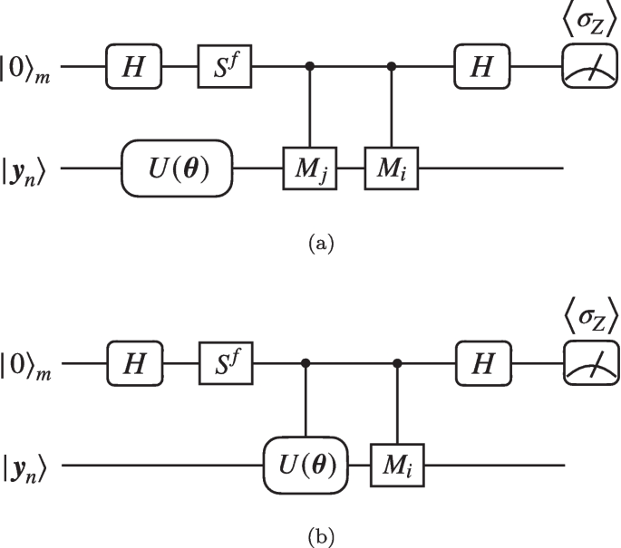
Quantum circuits for evaluating the values of a $B_{ij} = \langle {\varvec{y}_{n} | U^\dagger (\varvec{\theta }) {\varvec{M}}_i {\varvec{M}}_j U(\varvec{\theta }) | \varvec{y}_n}\rangle$ and b $\varvec{\gamma }_{i} = \langle {\varvec{y}_{n} | U^\dagger (\varvec{\theta }) {\varvec{M}}_i | \varvec{y}_{n}}\rangle$ based on the measurement results of the auxiliary qubit. Here the controlled gates are applied when the auxiliary qubit is on $|{1}\rangle _{m}$

In the circuit for computing $B_{ij}$, as shown in Fig. 2a, the Hadamard test [44] is employed, which requires one more auxiliary qubit $|{0}\rangle _m$. $S = \text {diag}(1, \textrm{i})$ is the phase shift gate and the flag f is either 0 or 1, determining whether the real part or the imaginary part of $B_{ij}$ is to be evaluated. The probability of obtaining $+1$ when we perform $\sigma _{z}$ measurement on the auxiliary qubit is

$$\begin{aligned} \Pr \nolimits _{f}(\sigma _{z} = +1)&= \frac{1}{4} \Big [2 + \textrm{i}^f \langle {\varvec{y}_{n} | U^{\dagger }(\varvec{\theta }) {\varvec{M}}_i {\varvec{M}}_j U(\varvec{\theta }) | \varvec{y}_{n}}\rangle \nonumber \\&\qquad + (-\textrm{i})^f \langle {\varvec{y}_{n} | U^{\dagger }(\varvec{\theta }) {\varvec{M}}_j {\varvec{M}}_i U(\varvec{\theta }) | \varvec{y}_{n}}\rangle \Big ] \nonumber \\&= \left\{ \begin{array}{ll} \frac{1}{2} \big (1 + \textrm{Re}\{B_{ij}\}\big ), &{} \quad f = 0; \\ \frac{1}{2} \big (1 - \textrm{Im}\{B_{ij}\}\big ), &{} \quad f = 1. \end{array}\right. \end{aligned}$$

(23)

Hence, we can evaluate $B_{ij}$ terms as

$$\begin{aligned} \textrm{Re}\{B_{ij}\} = \langle {\sigma _{z}}\rangle _{f = 0}, \textrm{Im}\{B_{ij}\} = -\langle {\sigma _{z}}\rangle _{f = 1}. \end{aligned}$$

(24)

When ${\varvec{A}}_i$s are Pauli-terms (as well as ${\varvec{M}}_is$), since $B_{ij}$ is essentially the expectation value of ${\varvec{M}}_i {\varvec{M}}_j$ of state $|{\varvec{y}_{n+1}(\varvec{\theta })}\rangle$, we can construct Hermitians from ${\varvec{M}}_i {\varvec{M}}_j$ and measure them on the quantum state directly, which does not require the auxiliary qubit $|{0}\rangle _{m}$ and is detailed in Appendix 1.

Similarly, circuit in Fig. 2b can output the real parts and imaginary parts of $\varvec{\gamma }_{i}$s respectively, according to

$$\begin{aligned} \Pr \nolimits _{f}(\sigma _{z} = +1)&= \frac{1}{4} \Big [2 + \textrm{i}^f \langle {\varvec{y}_{n} | {\varvec{M}}_i U(\varvec{\theta }) | \varvec{y}_{n}}\rangle \nonumber \\&\qquad + (-\textrm{i})^f \langle {\varvec{y}_{n} | U^{\dagger }(\varvec{\theta }) {\varvec{M}}_i | \varvec{y}_{n}}\rangle \Big ] \nonumber \\&= \left\{ \begin{array}{ll} \frac{1}{2} \big (1 + \textrm{Re}\{\varvec{\gamma }_{i}\}\big ), &{} \quad f = 0; \\ \frac{1}{2} \big (1 + \textrm{Im}\{\varvec{\gamma }_{i}\}\big ), &{} \quad f = 1, \end{array}\right. \end{aligned}$$

(25)

from which we have

$$\begin{aligned} \textrm{Re}\{\varvec{\gamma }_{i}\} = \langle {\sigma _{z}}\rangle _{f = 0}, \textrm{Im}\{\varvec{\gamma }_{i}\} = \langle {\sigma _{z}}\rangle _{f = 1}. \end{aligned}$$

(26)

Because of the symmetry of ${\varvec{B}}$, i.e., $B_{ij} = B_{ji}^*$, in general, $(3 + 4L) (3 + 4L + 1) / 2 = O(L^2)$ circuits for B and O(L) circuits for $\varvec{\gamma }$ are required. Note that the measurement is only applied on the auxiliary qubit under $\sigma _{z}$ bases, which is experimentally friendly.

2.4 Complexity of the algorithm

In our algorithm, two main approximations are adopted. One is using difference equations to reduce the original differential system, as in Eqs. (6), (7), and (8). The other is using Eq. (19) to avoid evaluating matrix inversion. Both are 2nd-order approximations, which implies that the local truncation error of this algorithm is $O({(\Delta t)^2})$. Therefore, our algorithm is a 1st-order finite-difference method, i.e., the global error $\epsilon$ is $O(\Delta t)$. As long as $\Delta t$ is sufficiently small, the algorithm solution will be close enough to the analytical result. The detailed derivations of local and global errors are provided in Appendices 2 and 3. In Appendix 4, we also discuss the error resulting from imperfect VQE optimization.

Qubit complexity of our algorithm is $\log _2 N + 2$ according to the circuit design described previously. This is the least qubits complexity required in quantum LDE solvers, since we need at least $\log _2 N$ qubits to encode N-dimensional vectors if there are no specific constraints on matrix ${\varvec{A}}$, e.g., ${\varvec{A}}$ being sparse. We need one auxiliary qubit to encode state $|{\varvec{y}}\rangle$, and another one for measuring elements of matrix B and vector $\varvec{\gamma }$ to evaluate the expectation of Hamiltonian in Eq. (9). Similar to our work, Berry et al. [36] solve Eq. (1) by discretizing them, but the converted difference equations at different time points are encoded in a single large linear system, indicating that more qubits are required for all time slices. Specifically, although qubit complexity of the algorithm is weakly affected by $\epsilon$, which is $O(\log (N \log (1/\epsilon )))$, the constant addition term in complexity is proportional to $\log (T\Vert {\varvec{A}}\Vert )$. Therefore, given a matrix ${\varvec{A}}$, the number of qubits required by the algorithm grows as the complete evolution time T gets longer. Recently, a work for solving d-dimension Poisson equation was also proposed [49]. Its spirit is similar to the discretizing method in [36], but it utilizes variational quantum algorithms to solve the encoded large linear system. Analogously, the algorithm for solving partial differential equations in [50] discretizes the variable domain with $2^n$ grid points and $2^m$ interpolation points and encodes $2^{n+m}$ function values directly into an $(n+m)$-qubit state which is constructed from a PQC. These algorithms require more qubits for finer discretization and hence higher accuracy, while our demand for qubit resources keeps constant for ordinary equations of certain differential order. Xin et al. [37] solve Eq. (1) by discretizing them using Taylor expansions of the analytical solution and require $O(\log (1/\epsilon ))$ more auxiliary qubits to perform the linear combination of unitaries.

Once all $n = T / \Delta t \sim O(1 / \epsilon )$ iterations are accomplished, the resulting circuit will be a series of PQC blocks:

$$\begin{aligned} \mathcal {U}&= \mathcal {U}^{(n)},\end{aligned}$$

(27)

$$\begin{aligned} \mathcal {U}^{(k)}&= U^{(k)}(\varvec{\theta }^{(k)}) \mathcal {U}^{(k-1)} = \prod _{i=k}^{1} U^{(i)}(\varvec{\theta }^{(i)}), \end{aligned}$$

(28)

where $\varvec{\theta }^{(k)} = (\varvec{\tau }^{(k)}, \varvec{\Omega }^{(k)})$. With reference to the structure of our ansatz, we can conclude that the gate complexity of the finally trained circuit $\mathcal {U}$ is $O(\frac{1}{\epsilon } n_q) = O(\frac{1}{\epsilon } \log N)$, which has the same logarithmic dependence on the system dimension N as existing algorithms. However, the dependence on $\epsilon$ is not optimal. We owe this to the balance between space complexity and time complexity of our LDE algorithms. Besides, $\mathcal {U}$ can restore the complete dynamical process of system evolution: we can extract the sub-circuits of $i \sim j$ slices in $\mathcal {U}$ for arbitrary i, j, and the yielded sub-series $\prod _{k=j}^{i} U^{(k)}$ reflects the evolution of $\varvec{y}(t)$ during time interval $[i \Delta t, j \Delta t]$. Moreover, if only the final solution $|{\varvec{y}(T)}\rangle$ but not the detailed evolution process is of our interest, we can check the length of $\mathcal {U}^{(i)}$ before each time step, and if there are more than $n_g$ gates, circuit optimization technologies in [55] can be employed to compress them into $n_g$ gates. Therefore, in the final circuit $\mathcal {U}^{(n)}$ the number of quantum gates will also be limited in $O(n_g)$. Here $n_g$ is a hyperparameter that should be determined with the compress fidelity guaranteed.

An estimation of the number of queries to quantum gates during the entire training process is provided in Appendix 5. It is worth noting that in order to make approximation (19) effective, $\Delta t$ must be restricted by $\Vert (\Delta t {\varvec{A}})^2\Vert \ll \Vert \Delta t {\varvec{A}}\Vert$. Therefore, we can select a $\Delta t$ satisfying $\Delta t \ll 1 / \Vert {\varvec{A}}\Vert$, where $\Vert {\varvec{A}}\Vert$ is the 2-norm of ${\varvec{A}}$.

3 Example models

We apply our algorithm to several linear differential equations to show how well it can solve classical systems dominated by equations as Eq. (1). We first consider an ordinary complex matrix

$$\begin{aligned} \varvec{A} = \left( \begin{array}{cc} -0.015-0.028 \textrm{i} &{} -0.963-0.928\textrm{i} \\ 0.105+0.251 \textrm{i} &{} -0.085-0.795 \textrm{i} \end{array}\right) \end{aligned}$$

(29)

with initial conditions

$$\begin{aligned} |{\varvec{x}_{0}}\rangle = \left( \begin{array}{c} 0 \\ \textrm{i} \end{array}\right) , \ |{\varvec{b}}\rangle = \frac{1}{\sqrt{2}} \left( \begin{array}{c} 1 \\ 1 \end{array}\right) . \end{aligned}$$

(30)

We set the time interval as $\Delta t = 0.1$ and the number of time steps as $n = 100$, to get the solution at $T = 10$. At the end of i-th time step, we simulate the optimized PQC $\mathcal {U}^{(i)}$ and evaluate the overlap at $t = i \Delta t$ by

$$\begin{aligned} f_i {:=} |\langle {\varvec{x}_{\text {alg}}(i \Delta t) | \varvec{x}_{\text {ana}}(i \Delta t)}\rangle |. \end{aligned}$$

(31)

Here $|{\varvec{x}_{\text {alg}}(i \Delta t)}\rangle = |{\varvec{x}_{i}}\rangle$ is the output state of $\mathcal {U}^{(i)}$, and $|{\varvec{x}_{\text {ana}}(i \Delta t)}\rangle = |{\varvec{x}(i \Delta t)}\rangle$ is the normalized analytical solution. Meanwhile, overlaps between the output state of PQC and the final analytical solution $f_i^{\text {alg}} {:=} |\langle {\varvec{x}_{\text {ana}}(T) | \varvec{x}_{\text {alg}}(i \Delta t)}\rangle |$ and overlaps between the analytical solution at current time and the final analytical solution $f_i^{\text {ana}} {:=} |\langle {\varvec{x}_{\text {ana}}(T) | \varvec{x}_{\text {ana}}(i \Delta t)}\rangle |$ are also calculated. These metrics are also called fidelities, time evolution of which are shown in Fig. 3. From the curve of $f_i$ (red dashed line), we can see that our algorithm can effectively simulate the evolution of linear differential equations, keeping the instantaneous overlaps between the algorithm states and the corresponding analytical solutions higher than 98%. High instantaneous overlaps mean that our algorithm can keep high fidelities during the whole evolution process (i.e., in all intermediate time slices of [0, T]), while the high final value of overlap $f^{\text {alg}}_i$ indicates that the algorithm can obtain the ideal final result. Meanwhile, by comparing the complete curves of $f^{\text {alg}}_i$ and $f^{\text {ana}}_i$ in Fig. 3 (deep blue solid line and light blue dashed line respectively), we can conclude that our algorithm can keep consistent with the analytical metric values during the whole evolution process.

Fig. 3

Time evolution of fidelities (i.e., overlaps) for linear differential system defined by Eqs. (29) and (30). Here $|{\varvec{x}_{\text {alg}}(t)}\rangle$ and $|{\varvec{x}_{\text {ana}}(t)}\rangle$ stand for the solution given out by the PQC in our algorithm (abbr. “alg”) and the analytical solution (abbr. “ana”) at time t respectively. The element values of the state vectors at the beginning of evolution $(t = \Delta t = 0.1)$ and at the end of evolution $(t = T = 10)$ are displayed in the lower-left and upper-right subfigures, where $x_{i} (i=0,1)$ is the i-th element of $|{\varvec{x}}\rangle$

Moreover, in order to demonstrate the applicability of our algorithm under different initial conditions, we keep the definition of ${\varvec{A}}$ as Eq. (29) and simulate the algorithm to solve equations with $|{\varvec{x}_0}\rangle$ and $|{\varvec{b}}\rangle$ being

$$\begin{aligned} |{\varvec{x}_{0}}\rangle&= \cos \frac{\alpha }{2} |{0}\rangle + \sin \frac{\alpha }{2} |{1}\rangle ,\end{aligned}$$

(32)

$$\begin{aligned} |{\varvec{b}}\rangle&= \cos \frac{\beta }{2} |{0}\rangle + \sin \frac{\beta }{2} |{1}\rangle , \end{aligned}$$

(33)

where $\alpha = n\pi /5,\ \beta = m\pi /5,\ n, m \in \{0, 1, \cdots , 5\}$. We set the target time $T = 5$ and the time step $\Delta t = 0.1$. By varying the values of n and m, we calculate the difference between the final overlap $|\langle {\varvec{x}(T) | \varvec{x}_{N}}\rangle |$ and the ideal expectation, as shown in Fig. 4. The average value of final errors over all initial conditions is less than 0.0014, which means that the feasibility of our algorithm can still be maintained under different initial conditions.

Fig. 4

The errors of the final optimization results under different initial conditions of the differential system defined by Eq. (29)

Also, for the purpose of studying the algorithm performance under different values of time step $\Delta t$, the most important hyperparameter, we keep the conditions in Eq. (29) and Eq. (30) unchanged, while we set the evolution time $T = 10$, and tune $\Delta t$ from 0.05 to 0.95. For each $\Delta t$, we calculate the averaged fidelity at i-th step by

$$\begin{aligned} \mathcal {F}_{i; \Delta t} = \frac{1}{i} \sum _{j = 0}^{i} |\langle {\varvec{x}(T = j \Delta t) | \varvec{x}_{j}}\rangle |, \end{aligned}$$

(34)

which characterizes the overall precision of our algorithm during the whole training process. With discrete $\mathcal {F}_{i; \Delta t}$ data collected, three-dimensional interpolation based on multi-quadric radial basis function is performed, generating an interpolation function $\mathcal {F}(T, \Delta t)$ in the domain $[0, 10]_{T} \times [0.05, 0.95]_{\Delta t}$, which is plotted as the surface in Fig. 5. It is clear that if evolution time T or time step $\Delta t$ takes small value, our algorithm can produce solution state at high fidelity. As $\Delta t$ increases, the fidelities decline faster in the training process, which can be concluded from the slope towards large T-large $\Delta t$ direction in Fig. 5. In general, we can define an algorithm-effective area in parameter space satisfying $0< T \Delta t < \delta$, where $\delta$ is a fidelity-related parameter and a smaller value of $T \Delta t$ can lead to a better optimization result.

Fig. 5

Time averaged fidelities in training processes for different $\Delta t$. The target differential system is defined by Eqs. (29) and (30). Yellow dots are the original $\mathcal {F}_{i; \Delta t}$ data points. The three dimensional surface represents the interpolation function $\mathcal {F}(T, \Delta t)$. The square contour figure in the T-$\Delta t$ plane is the projection of $\mathcal {F}(T, \Delta t)$ surface

4 Applications

Above we have discussed the algorithm with an ordinary complex matrix from the perspective of mathematics and demonstrate the feasibility of our scheme under different parameter conditions. In this section, we apply our algorithm to the dynamical simulation of different real physical processes.

4.1 One-dimensional harmonic oscillator

The first physical model is the one-dimensional harmonic oscillator, whose displacement x(t) is governed by a second order differential equation:

$$\begin{aligned} \left\{ \begin{array}{l} \textrm{d}ot{x} + \omega ^2 x = 0, \\ x(0) = x_0, \\ \dot{x}(0) = x_0', \end{array}\right. \end{aligned}$$

(35)

where the intrinsic frequency $\omega$ only depends on the system. This equation can be converted into first order differential equations by introducing variable substitution $x_1 = x,\ x_2 = \dot{x}$. Therefore we have:

$$\begin{aligned} \left\{ \begin{array}{l} \dot{x}_2 + \omega ^2 x_1 = 0, \\ \dot{x}_1 = x_2, \\ x_1(0) = x_0, \\ x_2(0) = x_0'. \end{array}\right. \end{aligned}$$

(36)

We define a vector $\varvec{x}(t) = (x_1(t), x_2(t))^{\textrm{T}}$, and write it in the form of Eq. (1) and Eq. (2) as

$$\begin{aligned} \dot{\varvec{x}} = \left( \begin{array}{cc} 0 &{} 1 \\ -\omega ^2 &{} 0 \end{array}\right) \varvec{x}, \quad \varvec{x}(0) = \left( \begin{array}{c} x_0 \\ x_0' \end{array}\right) , \end{aligned}$$

(37)

which has an analytical solution:

$$\begin{aligned}&\varvec{x}(t) = \left( \begin{array}{c} x_0 \cos \omega t + \frac{x_0'}{\omega } \sin \omega t \\ -\omega x_0 \sin \omega t + {x_0'} \cos \omega t \end{array}\right) . \end{aligned}$$

(38)

We tested our algorithm for $\omega = 1.5$, and the initial conditions are $\varvec{x}(0) = (0, 1)^{\textrm{T}}, \varvec{b} = \varvec{0}$, which corresponds to the motion of a one-dimensional harmonic oscillator initially located at the coordinate origin with unit velocity. We set the time step $\Delta t = 0.1$. Our algorithm produces vectors highly consistent with analytical solutions. Note that the algorithm vectors are normalized, and the normalization factor c(t) can be determined by

$$\begin{aligned} c(t)&= \sqrt{x^{2}(t) + \dot{x}^{2}(t)} \end{aligned}$$

(39)

$$\begin{aligned}&= \left\{ \begin{array}{ll} \sqrt{2 E_0 \left[ \frac{1 + r(t)}{\omega ^2 + r(t)}\right] }, &{} \quad x_1(t) \ne 0; \\ \sqrt{2 E_0} &{} \quad x_1(t) = 0, \end{array}\right. \end{aligned}$$

(40)

where $E_0 = (\dot{x}^2(t) + \omega ^2 x^2(t)) / 2 \equiv ({x}_{0}^{\prime 2} + \omega ^2 x_0^2) / 2$ is the constant total energy if we assume the oscillator has unit mass, $r(t) = |x_2(t)/x_1(t)|^2 = |\bar{x}_2(t)/\bar{x}_1(t)|^2$ is the ratio of the probabilities for the work qubit at different states, and $\bar{x}_i(t) = x_i(t) / c(t) \ (i = 1,2)$. Therefore, the kinetic energy and the potential energy are evaluated as

$$\begin{aligned} E_{\textrm{p}} = \frac{1}{2} \omega ^2 c^2(t) |\bar{x}_1(t)|^2, \quad E_{\textrm{k}} = \frac{1}{2} c^2(t) |\bar{x}_2(t)|^2, \end{aligned}$$

(41)

and their evolution with time is shown in Fig. 6, which displays a behavior of sine functions with period $\sim 2\pi /3$ as expected in theory. It can be seen that the error of energy accumulates with time, which is a natural result of finite difference method according to the discussion in Section 2.4 and Appendix 3.

Such an example for solving second order differential equation shows that our algorithm can be applied to find solutions to those higher-order differential equations by converting them into first-order linear differential equations.

Fig. 6

a Time evolution of potential energy and kinetic energy for the one dimensional harmonic oscillator. b The energy difference between analytical (abbr. “ana”) and algorithm (abbr. “alg”) results. c The element values of the final state vectors (at $T = 10$) corresponding to analytical evaluation and algorithm solution

4.2 Non-Hermitian systems

In this part, we discuss the application of our algorithm to the dynamical simulation of non-Hermitian systems with $\mathcal{P}\mathcal{T}$-symmetry. In 1998, Bender found that Hamiltonians satisfying joint parity (spatial reflection) symmetry $\mathcal {P}$ and time reversal symmetry $\mathcal {T}$, instead of Hermiticity, can still have real eigenvalues. When the Hamiltonian commutes with the joint $\mathcal{P}\mathcal{T}$ operator, it is classified as a $\mathcal{P}\mathcal{T}$-symmetric Hamiltonian. If eigenstates of the $\mathcal{P}\mathcal{T}$-symmetric Hamiltonian are also the eigenstates of $\mathcal{P}\mathcal{T}$ operator, $\mathcal{P}\mathcal{T}$-symmetry is unbroken, while the symmetry is broken conversely [56]. The transition between these two phases in parameter space happens at so-called exceptional points or branch points [56, 57]. There are many novel physical phenomena shown up in this kind of systems, such as the violation of no-signaling principle [58], the symmetry breaking transition [59], $\mathcal{P}\mathcal{T}$-symmetric quantum walk, and characters of exceptional point [60]. Especially, it is shown that the entanglement can be restored by a local $\mathcal{P}\mathcal{T}$-symmetric operation [61,62,63], which can not be observed in the traditional Hermitian quantum mechanics.

We consider a coupled two-mode system (coupling strength s) with balanced gain and loss ($\lambda s$), which can be regarded as a $\mathcal{P}\mathcal{T}$-symmetric qubit with Hamiltonian:

$$\begin{aligned} H_{\mathcal{P}\mathcal{T}} = s (\sigma _{x} + \textrm{i} \lambda \sigma _{z}) \end{aligned}$$

(42)

where $\sigma _{i}\ (i=x,y,z)$ are Pauli matrices and the positive parameter $\lambda$ represents the degree of non-Hermiticity in the system. The energy gap of the Hamiltonian $\omega =2s\sqrt{1-\lambda ^{2}}$ will be real as long as $\lambda <1$, meaning that the $\mathcal{P}\mathcal{T}$ symmetry is unbroken, in which cases the Hamiltonian keeps invariant under $\mathcal{P}\mathcal{T}$ transformation: $(\mathcal{P}\mathcal{T})H_{\mathcal{P}\mathcal{T}}(\mathcal{P}\mathcal{T})^{-1}=H_{\mathcal{P}\mathcal{T}}$, where the operator $\mathcal {P}=\sigma _{x}$ and $\mathcal {T}$ corresponds to the operation of complex conjugation. On the other hand, $\lambda > 1$ will lead to a broken phase with a transition at exceptional point $\lambda _{\textrm{ep}}=1$.

Suppose that there is another qubit, which is entangled with the $\mathcal{P}\mathcal{T}$-symmetric qubit and they form Bell state $(|{01}\rangle + |{10}\rangle )/\sqrt{2}$ initially. To investigate the dynamic process of the two-qubit non-Hermitian system, we take $\varvec{x}(t)$ to represent the quantum states. Comparing the evolution equation of this non-Hermitian quantum system with Eq. (1), we can determine that

$$\begin{aligned} {\varvec{A}} = -\textrm{i} H_{\mathcal{P}\mathcal{T}} \otimes {\varvec{I}}, \varvec{x}_0 = \frac{1}{\sqrt{2}} (0, 1, 1, 0)^{\textrm{T}}, \varvec{b} = (0, 0, 0, 0)^{\textrm{T}}. \end{aligned}$$

(43)

Here we take $\hbar = 1$ for simplicity, and s is set to be one. We use our algorithm to solve the differential equations of state evolution and monitor the degree of entanglement by concurrence [64], which is defined as

$$\begin{aligned} C(\rho ) = \max \{ 0,\sqrt{\mu _{1}}-\sqrt{\mu _{2}}-\sqrt{\mu _{3}}-\sqrt{\mu _{4}} \}, \end{aligned}$$

(44)

where $\rho =|{\varvec{x}(t)}\rangle \langle {\varvec{x}(t)}|$ is the density matrix of the two-qubit system, and $\mu _{i}$s are the eigenvalues of $\rho (\sigma _{y} \otimes \sigma _{y})\rho ^{*}(\sigma _{y} \otimes \sigma _{y})$ in descending order.

The numerical simulation results are shown in Fig. 7 and the configuration of simulation is detailed in Appendix 6. We can conclude that the entanglement decays exponentially to zero in the symmetry-broken phase ($\lambda = 2.0$), while the entanglement oscillates with time in the unbroken phase ($\lambda = 0.5$), indicating the entanglement restoration phenomenon induced by the local $\mathcal{P}\mathcal{T}$-symmetric system. As for the case at $\lambda = 0.99$, the temporal period of concurrence becomes so long that the evolution displays a decay-like behavior in limited time, conforming to the properties of near-exceptional points. These results are consistent with theoretical expectations.

Fig. 7

a Evolution of concurrence in the two-qubit entangled system with local $\mathcal{P}\mathcal{T}$-symmetry under different degree of non-Hermiticity. b The errors between analytical and algorithm results

In this example, the evolutionary process restored by our algorithm reveals interesting physics that is unable to be observed in the traditional Hermitian quantum mechanics. That is the increase of entanglement during a specific time interval ($t \in [1.8, 3.0]$) in the unbroken phase of $\mathcal{P}\mathcal{T}$-symmetry. If we just concentrate on the initial state ($t = 0$) and the final state ($t = 3.0$), only the relative reduction in concurrence can be concluded, and we cannot observe the entanglement restoration process [61].

5 Conclusion

In this work, we propose a hybrid quantum-classical algorithm for solving linear differential equations. The spirit of the algorithm is a first-order finite difference method, with solution vectors well encoded into quantum states. For an N-dimension system, our algorithm only requires one auxiliary qubit and $\log N$ qubits to encode the solution, and another auxiliary qubit to assist in measuring Hamiltonian expectations, which is optimal compared with the previous works. The gate complexity is also logarithmic in N, presenting similar dependence on system dimension as existing algorithms. We demonstrate the algorithm with a general differential system and present its effectiveness and robustness under different initial conditions and hyperparameters. Furthermore, we apply the algorithm to the dynamical simulation of different physical processes, including a one-dimensional harmonic oscillator system and $\mathcal{P}\mathcal{T}$-symmetric non-Hermitian systems. Our work provides a new scheme for solving linear differential equations with NISQ devices and the protocol can also be demonstrated on practical quantum computation platforms. It is worth mentioning that the qubit coupled-cluster method is employed in our framework as the VQE sub-program for solving ground state problems. However, it is still an open question to choose more adequate eigensolvers for specific systems and we leave it in future works.

Appendices

Appendix 1. Another measurement scheme for $B_{ij}$ when ${\varvec{A}}_i$s are Pauli-terms

When ${\varvec{A}}_i$s are Pauli-terms, ${\varvec{M}}_i$s in Eq. (21) are Pauli-terms as well. Note that $B_{ij} = \langle {\varvec{y}_{n+1}(\varvec{\theta }) | {\varvec{M}}_i {\varvec{M}}_j | \varvec{y}_{n+1}(\varvec{\theta })}\rangle$ is the expectation value of ${\varvec{M}}_i {\varvec{M}}_j$ of quantum state $|{\varvec{y}_{n+1}(\varvec{\theta })}\rangle$. We define two operators as follows:

$$\begin{aligned} {\varvec{J}}_{ij}&= \frac{{\varvec{M}}_i {\varvec{M}}_j + {\varvec{M}}_j {\varvec{M}}_i}{2},\end{aligned}$$

(45)

$$\begin{aligned} {\varvec{K}}_{ij}&= \frac{{\varvec{M}}_i {\varvec{M}}_j - {\varvec{M}}_j {\varvec{M}}_i}{2\textrm{i}}, \end{aligned}$$

(46)

which satisfy ${\varvec{M}}_i {\varvec{M}}_j = {\varvec{J}}_{ij} + \textrm{i} {\varvec{K}}_{ij}$. When ${\varvec{M}}_i$s are Pauli-terms, it is direct to derive that ${\varvec{J}}_{ij}$ and ${\varvec{K}}_{ij}$ are both Hermitian and hence observables. Therefore, we can measure the expectation values of them on state $|{\varvec{y}_{n+1}(\varvec{\theta })}\rangle$ without the requirement for an auxiliary qubit as in Fig. 2a, and obtain $B_{ij}$ via $\langle {{\varvec{M}}_i {\varvec{M}}_j}\rangle = \langle {{\varvec{J}}_{ij}}\rangle + \textrm{i} \langle {{\varvec{K}}_{ij}}\rangle$.

Appendix 2. Local truncation error

According to the notations in the main text, the analytical state vector in the $(n + 1)$-th iteration is $\varvec{y}({t_{n + 1}})$, and the corresponding algorithm estimation is $\varvec{y}_{n + 1}$. When evaluting the local truncation error of a certain step, we assume that our algorithm gives out an accurate state in the previous step, i.e., $\varvec{y}_{n} = \varvec{y}(t_n)$. For the analytical vector, we have

$$\begin{aligned} \varvec{x}(t_{n + 1})&= \textrm{e}^{{\varvec{A}} \Delta t} \varvec{x}_{n} + (\textrm{e}^{{\varvec{A}} \Delta t} - {\varvec{I}}_N) {\varvec{A}}^{-1} \varvec{b} \end{aligned}$$

(47)

$$\begin{aligned}&= [{\varvec{I}}_N + {\varvec{A}} \Delta t + O({(\Delta t)^2})] \varvec{x}_{n} + [\Delta t + O({(\Delta t)^2})] \varvec{b}, \end{aligned}$$

(48)

$$\begin{aligned} \Vert \varvec{x}(t_{n + 1})\Vert&= \Vert \varvec{x}(t_{n})\Vert \left[ 1 + \frac{1}{2 \Vert \varvec{x}(t_{n})\Vert ^2} \Big (\varvec{x}^{\dagger }(t_n) ({\varvec{A}} \varvec{x}(t_{n}) + \varvec{b}) + \mathrm {h.c.}\Big ) \Delta t + O({(\Delta t)^2})\right] ,\\ \Vert \varvec{y}(t_{n + 1})\Vert&= \sqrt{\Vert \varvec{x}(t_{n+1})\Vert ^2 + \Vert \varvec{b}\Vert ^2}\nonumber \\&= \Vert \varvec{y}(t_{n})\Vert \left\{ 1 + \frac{1}{2\Vert \varvec{y}(t_{n})\Vert ^2} \left[ \varvec{x}^{\dagger }(t_{n}) ({\varvec{A}} \varvec{x}(t_{n}) + \varvec{b}) + \mathrm {h.c.} \right] \Delta t + O({(\Delta t)^2})\right\} , \end{aligned}$$

(49)

$$\begin{aligned} |{\varvec{y}(t_{n + 1})}\rangle&= \frac{1}{\Vert \varvec{y}(t_{n + 1})\Vert } \left( \begin{array}{c} \varvec{x}(t_{n + 1}) \\ \varvec{b} \end{array}\right) , \end{aligned}$$

(50)

where $\varvec{y}(t_{n}) = (\varvec{x}(t_{n}); \varvec{b})$.

As for the algorithm vector, if we ignore the error in finding the ground state of Hamiltonian, following relations hold:

$$\begin{aligned} \varvec{x}_{n + 1}&= ({\varvec{I}}_N + {\varvec{A}} \Delta t) \varvec{x}_{n} + \Delta t \varvec{b}, \end{aligned}$$

(51)

$$\begin{aligned} \Vert \varvec{x}_{n + 1}\Vert&\sim \Vert \varvec{x}(t_{n + 1})\Vert \quad (\text {2nd order}), \end{aligned}$$

(52)

$$\begin{aligned} \Vert \varvec{y}_{n + 1}\Vert&\sim \Vert \varvec{y}(t_{n + 1})\Vert \quad (\text {2nd order}), \end{aligned}$$

(53)

$$\begin{aligned} |{\varvec{y}_{n + 1}}\rangle&= \frac{1}{\Vert \varvec{y}_{n + 1}\Vert } \left( \begin{array}{c} \varvec{x}_{n + 1} \\ \varvec{b} \end{array}\right) \sim |{\varvec{y}(t_{n + 1})}\rangle \quad (\text {2nd order}), \end{aligned}$$

(54)

However, approximation on matrix ${\varvec{M}}$ is adopted in ground state finding according to Eq. (19). Here we denote the approximate matrix by $\tilde{{\varvec{M}}}$. Hence, the solution of our algorithm should be given out by

$$\begin{aligned} \tilde{\varvec{y}}_{n+1}&= \tilde{{\varvec{M}}}^{-1} \varvec{y}_{n} = \tilde{{\varvec{M}}}^{-1} \left( \begin{array}{c} \varvec{x}(t_{n}) \\ \varvec{b} \end{array}\right) \end{aligned}$$

(55)

$$\begin{aligned}&= \left( \begin{array}{c} ({\varvec{I}}_N - {\varvec{A}} \Delta t)^{-1} \varvec{x}(t_n) + \Delta t\varvec{b} \\ \varvec{b} \end{array}\right) \end{aligned}$$

(56)

$$\begin{aligned}&= \left( \begin{array}{c} \varvec{x}(t_n) + ({\varvec{A}} \varvec{x}(t_n) + \varvec{b}) \Delta t + O({(\Delta t)^2}) \\ \varvec{b} \end{array}\right) \end{aligned}$$

(57)

$$\begin{aligned}&= \left( \begin{array}{c} \varvec{x}_{n + 1} + O({(\Delta t)^2}) \\ \varvec{b} \end{array}\right) = \varvec{y}_{n + 1} + O({(\Delta t)^2}) \end{aligned}$$

(58)

$$\begin{aligned}&= \varvec{y}(t_{n + 1}) + O({(\Delta t)^2}), \end{aligned}$$

(59)

$$\begin{aligned} |{\tilde{\varvec{y}}_{n+1}}\rangle&= \frac{\tilde{{\varvec{M}}}^{-1} \varvec{y}_{n}}{\Vert \tilde{{\varvec{M}}}^{-1} \varvec{y}_{n}\Vert } \end{aligned}$$

(60)

$$\begin{aligned}&= \frac{\varvec{y}_{n + 1} + O({(\Delta t)^2})}{\Vert \varvec{y}_{n + 1} + O({(\Delta t)^2})\Vert } \end{aligned}$$

(61)

$$\begin{aligned}&= \frac{\varvec{y}_{n + 1} + O({(\Delta t)^2})}{\Vert \varvec{y}_{n + 1}\Vert }[1 + O({(\Delta t)^2})] \end{aligned}$$

(62)

$$\begin{aligned}&= |{\varvec{y}_{n + 1}}\rangle + O({(\Delta t)^2}) \end{aligned}$$

(63)

$$\begin{aligned}&= |{\varvec{y}(t_{n + 1})}\rangle + O({(\Delta t)^2}). \end{aligned}$$

(64)

The error of $|{\tilde{\varvec{y}}_{n+1}}\rangle$ is a 2nd order infinitesimal of $\Delta t$ compared with $|{\varvec{y}(t_{n + 1})}\rangle$. Then, we have

$$\begin{aligned}&\frac{\tilde{\varvec{x}}_{n + 1}}{\Vert \tilde{\varvec{y}}_{n + 1}\Vert } - \frac{\varvec{x}(t_{n + 1})}{\Vert \varvec{y}(t_{n + 1})\Vert } \end{aligned}$$

(65)

$$\begin{aligned} = {}&\frac{1}{\Vert \tilde{\varvec{y}}_{n + 1}\Vert } \left[ \tilde{\varvec{x}}_{n + 1} - \varvec{x}(t_{n + 1}) \frac{\Vert \tilde{\varvec{y}}_{n + 1}\Vert }{\Vert \varvec{y}(t_{n + 1})\Vert }\right] \end{aligned}$$

(66)

$$\begin{aligned} = {}&\frac{1}{\Vert \tilde{\varvec{y}}_{n + 1}\Vert } \left[ \tilde{\varvec{x}}_{n + 1} - \varvec{x}(t_{n + 1}) + O({(\Delta t)^2})\right] . \end{aligned}$$

(67)

From Eq. (65), we know that the difference above is $O({(\Delta t)^2})$, which indicates that

$$\begin{aligned} \tilde{\varvec{x}}_{n + 1} - \varvec{x}(t_{n + 1}) = O({(\Delta t)^2}). \end{aligned}$$

(68)

In summary, the local truncation error of our algorithm is

$$\begin{aligned} l_{n + 1}&= |{\tilde{\varvec{y}}_{n + 1}}\rangle - |{\varvec{y}(t_{n + 1})}\rangle = O({(\Delta t)^2}). \end{aligned}$$

(69)

Appendix 3. Global error

Global error describes the accumulation effect of local errors. Since ${\varvec{A}}$ is diagonalizable, we assume that ${\varvec{A}} = {\varvec{F}}^{-1} {\varvec{\Lambda }} {\varvec{F}}$ where ${\varvec{\Lambda }} = \text {diag}(\lambda _1, \cdots , \lambda _N)$ is the diagonal matrix composed of the eigenvalues of ${\varvec{A}}$. Firstly, consider the i-th element of $\varvec{x}(t_{n + 1}) = \textrm{e}^{{\varvec{A}} \Delta t} \varvec{x}(t_{n}) + (\textrm{e}^{{\varvec{A}} \Delta t} - {\varvec{I}}_N) {\varvec{A}}^{-1} \varvec{b}$, which can be expressed as a first-order Taylor series with Lagrangian remainder as follows (where Einstein summation convention is adopted):

$$\begin{aligned} {x}^{(i)}(t_{n+1})&= ({\varvec{F}}^{-1})_{ij} \textrm{e}^{\lambda _j \Delta t} F_{jk} x^{k}(t_n) + ({\varvec{F}}^{-1})_{ij} \frac{\textrm{e}^{\lambda _j \Delta t} - 1}{\lambda _j} F_{jk} b_k \nonumber \\&= ({\varvec{F}}^{-1})_{ij} \left[ 1 + \lambda _j \Delta t + \frac{1}{2} \textrm{e}^{\lambda _j \xi _j} (\lambda _j \Delta t)^2\right] F_{jk} x^{(k)}(t_n) \nonumber \\&\hspace{2em} + ({\varvec{F}}^{-1})_{ij} \left[ \Delta t + \frac{1}{2} \textrm{e}^{\lambda _j \xi _j} \lambda _j {(\Delta t)^2}\right] F_{jk} b^{(k)} \nonumber \\&= \left[ \delta _{ik} + ({\varvec{F}}^{-1} {\varvec{\Lambda }} {\varvec{F}})_{ik} \Delta t + \frac{1}{2} ({\varvec{F}}^{-1} \textrm{e}^{{\varvec{\Lambda }}'} {\varvec{\Lambda }}^2 {\varvec{F}})_{ik}{(\Delta t)^2}\right] x^{(k)}(t_n) \nonumber \\&\hspace{2em} + \left[ \delta _{ik} \Delta t + \frac{1}{2} ({\varvec{F}}^{-1} \textrm{e}^{{\varvec{\Lambda }}'} {\varvec{\Lambda }} {\varvec{F}})_{ik} {(\Delta t)^2}\right] b^{(k)} \nonumber \\&= ({\varvec{I}}_N + {\varvec{A}} \Delta t)_{ik} x^{(k)}(t_n) + \Delta t b^{(i)} \nonumber \\&\hspace{2em} + \left[ \frac{1}{2} ({\varvec{F}}^{-1} \textrm{e}^{{\varvec{\Lambda }}'} {\varvec{F}} {\varvec{A}}^2)_{ik}{(\Delta t)^2}\right] x^{(k)}(t_n) + \left[ \frac{1}{2} ({\varvec{F}}^{-1} \textrm{e}^{{\varvec{\Lambda }}'} {\varvec{F}} {\varvec{A}})_{ik} {(\Delta t)^2}\right] b^{(k)}, \end{aligned}$$

(70)

where $\xi _i \in (0, \Delta t)$, ${\varvec{\Lambda }}' = \text {diag}(\lambda _1 \xi _1, \cdots , \lambda _N \xi _N)$. Combining all N components yields

$$\begin{aligned} \varvec{x}(t_{n+1})&= \left[ {\varvec{I}}_N + {\varvec{A}} \Delta t + \frac{1}{2} ({\varvec{F}}^{-1} \textrm{e}^{{\varvec{\Lambda }}'} {\varvec{F}} {\varvec{A}}^2) {(\Delta t)^2}\right] \varvec{x}(t_{n}) + \left[ \Delta t + \frac{1}{2} ({\varvec{F}}^{-1} \textrm{e}^{{\varvec{\Lambda }}'} {\varvec{F}} {\varvec{A}}) {(\Delta t)^2}\right] \varvec{b}. \end{aligned}$$

(71)

Let ${\varvec{M}}_1 = \frac{1}{2} ({\varvec{F}}^{-1} \textrm{e}^{{\varvec{\Lambda }}'} {\varvec{F}} {\varvec{A}}^2), \ {\varvec{M}}_2 = \frac{1}{2} ({\varvec{F}}^{-1} \textrm{e}^{{\varvec{\Lambda }}'} {\varvec{F}} {\varvec{A}})$, and $\kappa$ be the condition number of ${\varvec{F}}$, so

$$\begin{aligned} \Vert {\varvec{F}}^{-1} \textrm{e}^{{\varvec{\Lambda }}'} {\varvec{F}}\Vert&\le \kappa \Vert \textrm{e}^{{\varvec{\Lambda }}'}\Vert = \kappa \max _{i} \textrm{e}^{\xi _i \textrm{Re}\{\lambda _i\}} \le \kappa \textrm{e}^{T r_{\max }}, \end{aligned}$$

(72)

$$\begin{aligned} \Vert {\varvec{A}}\Vert&= \Vert {\varvec{F}}^{-1} {\varvec{\Lambda }} {\varvec{F}}\Vert \le \kappa \Vert {\varvec{\Lambda }}\Vert = \kappa \max _{i} |\lambda _i|, \end{aligned}$$

(73)

where $r_{\max } = \max _{i} \textrm{Re}\{\lambda _i\}$. Therefore,

$$\begin{aligned} \Vert {\varvec{M}}_1\Vert&\le \frac{1}{2} \kappa \textrm{e}^{T r_{\max }} \Vert {\varvec{A}}\Vert ^2, \end{aligned}$$

(74)

$$\begin{aligned} \Vert {\varvec{M}}_2\Vert&\le \frac{1}{2} \kappa \textrm{e}^{T r_{\max }} \Vert {\varvec{A}}\Vert . \end{aligned}$$

(75)

Meanwhile, $\varvec{x}(t)$ has bounded norm in the interval of [0, T]:

$$\begin{aligned} \Vert \varvec{x}(t)\Vert&\le \Vert \textrm{e}^{{\varvec{A}} T}\Vert \Vert \varvec{x}_0\Vert + \Vert (\textrm{e}^{{\varvec{A}} T} - {\varvec{I}}_N) {\varvec{A}}^{-1}\Vert \Vert \varvec{b}\Vert \nonumber \end{aligned}$$

(76)

$$\begin{aligned}&\le \textrm{e}^{\Vert {\varvec{A}}\Vert T} \Vert \varvec{x}_0\Vert + \frac{\textrm{e}^{\Vert {\varvec{A}}\Vert T} - 1}{\Vert {\varvec{A}}\Vert } \Vert \varvec{b}\Vert {{:=}} {M}_0 \end{aligned}$$

(77)

Note that the solution of our algorithm at $t = (n + 1) \Delta t$ should be

$$\begin{aligned} \varvec{x}_{n+1}&= [{\varvec{I}}_N + {\varvec{A}} \Delta t] \varvec{x}_{n} + \Delta t \varvec{b}. \end{aligned}$$

(78)

Combining all estimations above and defining $\varvec{\epsilon }_{n} = \varvec{x}(t_{n}) - \varvec{x}_{n}$, we can derive the upper bound of the global error at $t = T$ (hence $n + 1 = N = T / \Delta t$) as

$$\begin{aligned} \Vert \varvec{\epsilon }_{n+1}\Vert&\le \Vert {\varvec{I}}_N + {\varvec{A}} \Delta t\Vert \Vert \varvec{\epsilon }_{n}\Vert + \Vert {\varvec{M}}_1\Vert {(\Delta t)^2} {M}_0 + \Vert {\varvec{M}}_2\Vert {(\Delta t)^2} \Vert \varvec{b}\Vert \nonumber \\&\le (1 + \Vert {\varvec{A}}\Vert \Delta t) \Vert \varvec{\epsilon }_{n}\Vert + {M} {(\Delta t)^2} \nonumber \\&= (1 + \Vert {\varvec{A}}\Vert \Delta t)^{n + 1} \Vert \varvec{\epsilon }_0\Vert + \frac{{(1 + \Vert {\varvec{A}}\Vert \Delta t)}^{n+1} - 1}{1 + \Vert {\varvec{A}}\Vert \Delta t - 1} {M} {(\Delta t)^2} \nonumber \\&= T {M} \Delta t + O(\Delta t^3). \end{aligned}$$

(79)

Here the condition $\Vert \varvec{\epsilon }_0\Vert = 0$ is used, and factor M is a positive constant related to ${\varvec{A}}, T, \varvec{x}_0$ and $\varvec{b}$, whose upper bound can be estimated using Eqs. (75), (76), and (77):

$$\begin{aligned} M = \Vert {\varvec{M}}_1\Vert {M}_0 + \Vert {\varvec{M}}_2\Vert \Vert \varvec{b}\Vert \le \frac{1}{2} \kappa \textrm{e}^{T r_{\max }} \Vert {\varvec{A}}\Vert \textrm{e}^{\Vert {\varvec{A}}\Vert T} \left( \Vert {\varvec{A}}\Vert \Vert \varvec{x}_0\Vert + \Vert \varvec{b}\Vert \right) . \end{aligned}$$

(80)

So far we have proved that the global error of our algorithm is of 1st order of $\Delta t$.

Appendix 4. Error from imperfect VQE optimization

Apart from the truncation error intrinsic to finite difference method, the precision of the VQE sub-program employed in each evolution step also influences the error. Here we discuss it in detail.

Firstly, we express the solution obtained from the VQE sub-program of our algorithm in the i-th step as

$$\begin{aligned} |{\tilde{\varvec{y}}_{i}}\rangle = \frac{|{\varvec{y}_{i}}\rangle + \eta |{\varvec{y}_{i}^{\perp }}\rangle }{\sqrt{1 + \eta ^2}}, \end{aligned}$$

(81)

where $|{\varvec{y}_{i}}\rangle$ is the analytical ground state of Hamiltonian (9) (which is also the only eigenstate that corresponds to zero energy), $|{\varvec{y}_{i}^{\perp }}\rangle$ stands for a normalized quantum state that is perpendicular to $|{\varvec{y}_{i}}\rangle$, and the real number $\eta$ measures the deviation of our algorithm solution from the analytical solution.

For arbitrary state $|{\phi }\rangle$ in the subspace defined by ${\varvec{M}}^{-1} \mathcal {H}_{\perp } = \{{\varvec{M}}^{-1} |{\psi }\rangle | |{\psi }\rangle \in \mathcal {H}_{\perp }\}$, where $\mathcal {H}_{\perp } = \{|{\psi }\rangle | \langle {\psi | \varvec{y}_{i-1}}\rangle = 0\}$, we have

$$\begin{aligned} \langle {\phi | H | \phi }\rangle = \langle {\phi | {\varvec{M}}^{\dagger } ({\varvec{I}}_{2N} - |{\varvec{y}_{i-1}}\rangle \langle {\varvec{y}_{i-1}}|) {\varvec{M}} | \phi }\rangle = 1. \end{aligned}$$

(82)

We can express $|{\varvec{y}_{i}^{\perp }}\rangle$ as $\frac{1}{C} {\varvec{M}}^{-1} [\alpha |{\varvec{y}_{i - 1}}\rangle + \beta |{\varvec{y}_{i - 1}^{\perp }}\rangle ]$, where the state vector $|{\varvec{y}_{i - 1}^{\perp }}\rangle \in \mathcal {H}_{\perp }$ is normalized, coefficients $\alpha , \beta$ satisfy $|\alpha |^2 + |\beta |^2 = 1$, and C is the normalization factor of $|{\varvec{y}_{i}^{\perp }}\rangle$. From the following relationships

$$\begin{aligned}&\langle {{\varvec{y}}_{i}^{\perp } | {\varvec{y}}_{i}}\rangle = 0, \end{aligned}$$

(83)

$$\begin{aligned}&({\varvec{M}}^{-1})^{\dagger } {\varvec{M}}^{-1} = {\varvec{I}}_{2N} + O(\Delta t) \end{aligned}$$

(84)

we can derive that $\alpha = O(\Delta t),\ \beta = 1 + O({(\Delta t)^2}),\ C = \left[ \langle {\varvec{y}_{i - 1}^{\perp } | ({\varvec{M}}^{-1})^{\dagger } {\varvec{M}}^{-1} | \varvec{y}_{i - 1}^{\perp }}\rangle + O(\Delta t)\right] ^{1/2} = 1 + O(\Delta t)$. Therefore $|{{\varvec{y}}_{i}^{\perp }}\rangle = [{\varvec{M}}^{-1} |{\varvec{y}_{i - 1}^{\perp }}\rangle + O(\Delta t)] / (1 + O(\Delta t))$. As a result, we have the Hamiltonian expectation as

$$\begin{aligned} \delta = \langle {\tilde{\varvec{y}}_{i} | {H} | \tilde{\varvec{y}}_{i}}\rangle = \frac{\eta ^2 \langle {{\varvec{y}}_{i}^{\perp } | {H} | {\varvec{y}}_{i}^{\perp }}\rangle }{(1 + \eta ^2)} = \frac{\eta ^2}{(1 + \eta ^2)} \frac{1 + O(\Delta t)}{(1 + O(\Delta t))^2}\sim \eta ^2 (1 + O(\Delta t)). \end{aligned}$$

(85)

Hence, the error of our algorithm solution resulting from imperfect VQE optimization is

$$\begin{aligned} \epsilon _{\text {VQE}} = 1 - |\langle {{\varvec{y}}\rangle _{i} | \tilde{\varvec{y}}_{i}}| = 1 - \frac{1}{\sqrt{1 + \eta ^2}} \sim \frac{1}{2} \eta ^2 \sim \frac{1}{2} \delta \cdot (1 + O(\Delta t)). \end{aligned}$$

(86)

By choosing an appropriate VQE sub-program for a specific differential system, $\delta$ and the error $\epsilon _{\text {VQE}}$ can be reduced so that the state $|{\tilde{\varvec{y}}_{i}}\rangle$ in Eq. (81) can serve as a good approximation to $|{\varvec{y}_{i}}\rangle$. In our numerical simulation, we employ qubit coupled cluster method as our VQE sub-program (Section 2.2). In consequence, the expectation values of the Hamiltonian output from the optimized PQC in each step are reduced to be $5 \times 10^{-8} \sim 1.7 \times 10^{-4}$ averagely.

Taking the errors from truncation in finite difference method and imperfect VQE optimization into account, if we set the time step length $\Delta t$ to be $\sim \epsilon$ and select a suitable VQE sub-program that can output an energy expectation value of $\sim \epsilon ^2$, then the local error in each step due to difference approximation and imperfect VQE optimization will be $O({(\Delta t)^2})$, and the accumulated error is $O(\Delta t) \sim \epsilon$.

Appendix 5. Gate query complexity

As for general variational quantum algorithms, including those for solving linear differential equations and simulating general evolutionary process [48, 49, 65], it is not direct to derive an exact value of the time complexity, since it is strongly related with the trainability of the parameterized quantum circuit, the training strategy employed, and the specific configuration of the target function (or loss function) in the parameter space.

For the completeness of discussion, here we give out an asymptotic upper bound of the gate query complexity of our algorithm, i.e., the number of quantum gate queries in experiment. In classical computing, the time complexity is evaluated by the number of basic operations like adding, subtracting, and other arithmetic operations. Analogously, we take the gate query complexity as the metric of time complexity of our quantum algorithm.

Firstly, we concentrate on the optimization process of the i-th step ($t \in [i \Delta t, (i+1) \Delta t]$). Since we use qubit coupled cluster method as our VQE sub-program, $O( n_q^{l_p} \times L^2 i n_q \times n_q^2)$ gate queries are required for Pauli-term ranking, and at most $O( n_e \times (2 n_q + p) \times L^2 i (2 n_q + p))$ gate queries for VQE optimization (including evaluation of gradients if a gradient-based classical optimizer is employed), where $n_e$, the maximal number of training epochs in each time step, is a preset hyperparameter; $n_q$ is the number of qubits of the differential system; $l_p$ is the maximal number of qubits acted on by the selected Pauli-terms in QCC procedure; L is the number of unitaries in the decomposition of matrix ${\varvec{A}}$; and p is the number of Pauli-terms to be selected in QCC Pauli-ranking procedure (see Section 2.2). Here the factor of $L^2$ comes from the fact that we need to evaluate $O(L^2)$ elements of ${\varvec{B}}$ and O(L) elements of $\varvec{\gamma }$. Therefore, the time complexity of training the VQE sub-program for minimizing the expectation value of the Hamiltonian in the i-th step is $O(n_q^{l_p + 3} L^2 i)$, where constants and hyperparameters are omitted.

Then, we sum the complexities up for all $T/\Delta t$ steps. According to the discussions in Appendices 1, 2, and 3, $\Delta t \ge {\epsilon } / {(TM)}$, where $\epsilon$ is the error of the final state. As a result, we have the total gate query complexity through the complete algorithm procedure as:

$$\begin{aligned} O\bigg (\bigg (\frac{T}{\Delta t} L\bigg )^2 n_q^{l_p + 3}\bigg ) \le O\bigg (\bigg (\frac{L}{\epsilon }\bigg )^2 \log _2^{l_p + 3} N\bigg ). \end{aligned}$$

(87)

Since it is assumed that L has an order of $O(\text {poly} \log N)$, the total gate query complexity (hence the time complexity) of the entire algorithm is $O(\text {poly} \log N)$.

Appendix 6. Configurations for simulating non-Hermitian systems

We set the time limit $T = 3$ when simulating non-Hermitian systems using our algorithm. During the training process, L-BFGS-B [66, 67] optimizer is employed. For each $\lambda$, we select different hyperparameters to obtain good results, which are listed in Table 1. Here p is the number of Pauli entanglers used in each evolution step. In our experiment, we find that systems with larger $\lambda$ are easier to be simulated. Therefore, we initialize all parameters of QMF ansatzes to be zero for $\lambda = 2$, while for smaller $\lambda$s, QMF parameters are randomly sampled from a uniform distribution over their domains, which are $[0, \pi ]$ for $\theta _i$s and $[0, 2\pi ]$ for $\phi _i$s in Eq. (15). This random initialization strategy can avoid our parameters from being initialized on barren plateaus around the coordinate origin. Note that parameters of Pauli entanglers are always initialized as zeros. Also, we split the evolution process of $\lambda = 0.5$ system into two parts. This is because the turning point of the state is around $t \sim 1.8$, where the state change is not obvious. This leads to possible barren plateaus around the zero eigenvalue of Hamiltonian (9) and makes our algorithm harder to reach the global minimum. Hence, we use more Pauli entanglers to enhance our PQCs for $t > 1.8$. As a benefit, the time step $\Delta t$ can be larger than the value of $t \le 1.8$.

Table 1 Hyperparameters for simulating non-Hermitian systems with different $\lambda$s

References

J.J. Sakurai, Modern Quantum Mechanics, ed. by S. F. Tuan (Addison-Wesley Publishing Company, Boston, U.S., 1994)
C.I. Trombley, M.L. Ekiel-Jeżewska, Basic Concepts of Stokes Flows (Springer International Publishing, Cham, 2019), pp. 35–50. https://doi.org/10.1007/978-3-030-23370-9_2
J.D. Jackson, Classical electrodynamics (Wiley, New York, 1998)
M.A. Nielsen, I.L. Chuang, Quantum Computation and Quantum Information: 10th Anniversary Edition (Cambridge University Press, 2010). https://doi.org/10.1017/CBO9780511976667
D.R. Simon, On the power of quantum computation. SIAM J. Comput. 26(5), 1474–1483 (1997). https://doi.org/10.1137/S0097539796298637
G.L. Long, General quantum interference principle and duality computer. Commun. Theor. Phys. 45(5), 825–844 (2006). https://doi.org/10.1088/0253-6102/45/5/013
G.L. Long, Duality quantum computing and duality quantum information processing. Int. J. Theor. Phys. 50(4), 1305–1318 (2011). https://doi.org/10.1007/s10773-010-0603-z
S. Lloyd, Universal quantum simulators. Science 273(5278), 1073–1078 (1996)
X. Qiang, T. Loke, A. Montanaro, K. Aungskunsiri, X. Zhou, J.L. O’Brien, J.B. Wang, J.C.F. Matthews, Efficient quantum walk on a quantum processor. Nat. Commun. 7(1), 11511 (2016). https://doi.org/10.1038/ncomms11511
L.K. Grover, Quantum computers can search arbitrarily large databases by a single query. Phys. Rev. Lett. 79, 4709–4712 (1997). https://doi.org/10.1103/PhysRevLett.79.4709
G.L. Long, Grover algorithm with zero theoretical failure rate. Phys. Rev. A 64, 022307 (2001). https://doi.org/10.1103/PhysRevA.64.022307
D. Coppersmith, An approximate Fourier transform useful in quantum factoring, Tech. Rep. RC–19642 (IBM Research Division, New York, 1994).
P. Shor, in Proceedings 35th Annual Symposium on Foundations of Computer Science. Algorithms for quantum computation: discrete logarithms and factoring (1994), pp. 124–134. https://doi.org/10.1109/SFCS.1994.365700
P.W. Shor, Polynomial-time algorithms for prime factorization and discrete logarithms on a quantum computer. SIAM J. Comput. 26(5), 1484–1509 (1997). https://doi.org/10.1137/S0097539795293172
K. Kim, M.S. Chang, S. Korenblit, R. Islam, E.E. Edwards, J.K. Freericks, G.D. Lin, L.M. Duan, C. Monroe, Quantum simulation of frustrated ising spins with trapped ions. Nature 465(7298), 590–593 (2010). https://doi.org/10.1038/nature09071
X. Zhang, K. Zhang, Y. Shen, S. Zhang, J.N. Zhang, M.H. Yung, J. Casanova, J.S. Pedernales, L. Lamata, E. Solano, K. Kim, Experimental quantum simulation of fermion-antifermion scattering via boson exchange in a trapped ion. Nat. Commun. 9(1), 195 (2018). https://doi.org/10.1038/s41467-017-02507-y
J. Du, H. Li, X. Xu, M. Shi, J. Wu, X. Zhou, R. Han, Experimental implementation of the quantum random-walk algorithm. Phys. Rev. A 67, 042316 (2003). https://doi.org/10.1103/PhysRevA.67.042316
H. Tang, X.F. Lin, Z. Feng, J.Y. Chen, J. Gao, K. Sun, C.Y. Wang, P.C. Lai, X.Y. Xu, Y. Wang, L.F. Qiao, A.L. Yang, X.M. Jin, Experimental two-dimensional quantum walk on a photonic chip. Sci. Adv. 4(5), eaat3174 (2018). https://doi.org/10.1126/sciadv.aat3174
I.L. Chuang, N. Gershenfeld, M. Kubinec, Experimental implementation of fast quantum searching. Phys. Rev. Lett. 80, 3408–3411 (1998). https://doi.org/10.1103/PhysRevLett.80.3408
J.A. Jones, M. Mosca, R.H. Hansen, Implementation of a quantum search algorithm on a quantum computer. Nature 393(6683), 344–346 (1998). https://doi.org/10.1038/30687
P.G. Kwiat, J.R. Mitchell, P.D.D. Schwindt, A.G. White, Grover’s search algorithm: an optical approach. J. Mod. Opt. 47(2–3), 257–266 (2000). https://doi.org/10.1080/09500340008244040
J.L. Dodd, T.C. Ralph, G.J. Milburn, Experimental requirements for grover’s algorithm in optical quantum computation. Phys. Rev. A 68, 042328 (2003). https://doi.org/10.1103/PhysRevA.68.042328
A. Mandviwalla, K. Ohshiro, B. Ji, in 2018 IEEE International Conference on Big Data (Big Data). Implementing grover’s algorithm on the ibm quantum computers (2018), pp. 2531–2537. https://doi.org/10.1109/BigData.2018.8622457
C.Y. Lu, D.E. Browne, T. Yang, J.W. Pan, Demonstration of a compiled version of shor’s quantum factoring algorithm using photonic qubits. Phys. Rev. Lett. 99, 250504 (2007). https://doi.org/10.1103/PhysRevLett.99.250504
B.P. Lanyon, T.J. Weinhold, N.K. Langford, M. Barbieri, D.F.V. James, A. Gilchrist, A.G. White, Experimental demonstration of a compiled version of shor’s algorithm with quantum entanglement. Phys. Rev. Lett. 99, 250505 (2007). https://doi.org/10.1103/PhysRevLett.99.250505
E. Martín-López, A. Laing, T. Lawson, R. Alvarez, X.Q. Zhou, J.L. O’Brien, Experimental realization of shor’s quantum factoring algorithm using qubit recycling. Nat. Photonics 6(11), 773–776 (2012). https://doi.org/10.1038/nphoton.2012.259
B. Lu, L. Liu, J.Y. Song, K. Wen, C. Wang, Recent progress on coherent computation based on quantum squeezing. AAPPS Bull. 33(1), 7 (2023). https://doi.org/10.1007/s43673-023-00077-4
F. Zhang, J. Xing, X. Hu, X. Pan, G. Long, Coupling-selective quantum optimal control in weak-coupling nv-13c system. AAPPS Bull. 33(1), 2 (2023). https://doi.org/10.1007/s43673-022-00072-1
A.W. Harrow, A. Hassidim, S. Lloyd, Quantum algorithm for linear systems of equations. Phys. Rev. Lett. 103, 150502 (2009). https://doi.org/10.1103/PhysRevLett.103.150502
S. Wei, Z. Zhou, D. Ruan, G. Long, in 2017 IEEE 85th Vehicular Technology Conference (VTC Spring). Realization of the algorithm for system of linear equations in duality quantum computing (2017), pp. 1–4. https://doi.org/10.1109/VTCSpring.2017.8108698
S. Barz, I. Kassal, M. Ringbauer, Y.O. Lipp, B. Dakić, A. Aspuru-Guzik, P. Walther, A two-qubit photonic quantum processor and its application to solving systems of linear equations. Sci. Rep. 4(1), 6115 (2014). https://doi.org/10.1038/srep06115
J. Pan, Y. Cao, X. Yao, Z. Li, C. Ju, H. Chen, X. Peng, S. Kais, J. Du, Experimental realization of quantum algorithm for solving linear systems of equations. Phys. Rev. A 89, 022313 (2014). https://doi.org/10.1103/PhysRevA.89.022313
X.D. Cai, C. Weedbrook, Z.E. Su, M.C. Chen, M. Gu, M.J. Zhu, L. Li, N.L. Liu, C.Y. Lu, J.W. Pan, Experimental quantum computing to solve systems of linear equations. Phys. Rev. Lett. 110, 230501 (2013). https://doi.org/10.1103/PhysRevLett.110.230501
J. Wen, X. Kong, S. Wei, B. Wang, T. Xin, G. Long, Experimental realization of quantum algorithms for a linear system inspired by adiabatic quantum computing. Phys. Rev. A 99, 012320 (2019). https://doi.org/10.1103/PhysRevA.99.012320
D.W. Berry, High-order quantum algorithm for solving linear differential equations. J. Phys. A Math. Theor. 47(10), 105301 (2014). https://doi.org/10.1088/1751-8113/47/10/105301
D.W. Berry, A.M. Childs, A. Ostrander, G. Wang, Quantum algorithm for linear differential equations with exponentially improved dependence on precision. Commun. Math. Phys. 356(3), 1057–1081 (2017). https://doi.org/10.1007/s00220-017-3002-y
T. Xin, S. Wei, J. Cui, J. Xiao, I.n. Arrazola, L. Lamata, X. Kong, D. Lu, E. Solano, G. Long, Quantum algorithm for solving linear differential equations: theory and experiment. Phys. Rev. A 101, 032307 (2020). https://doi.org/10.1103/PhysRevA.101.032307
J.W.Z. Lau, K.H. Lim, H. Shrotriya, L.C. Kwek, Nisq computing: where are we and where do we go? AAPPS Bull. 32(1), 27 (2022). https://doi.org/10.1007/s43673-022-00058-z
A. Peruzzo, J. McClean, P. Shadbolt, M.H. Yung, X.Q. Zhou, P.J. Love, A. Aspuru-Guzik, J.L. O’Brien, A variational eigenvalue solver on a photonic quantum processor. Nat. Commun. 5(1), 4213 (2014). https://doi.org/10.1038/ncomms5213
J.R. McClean, J. Romero, R. Babbush, A. Aspuru-Guzik, The theory of variational hybrid quantum-classical algorithms. New J. Phys. 18(2), 023023 (2016). https://doi.org/10.1088/1367-2630/18/2/023023
A. Kandala, A. Mezzacapo, K. Temme, M. Takita, M. Brink, J.M. Chow, J.M. Gambetta, Hardware-efficient variational quantum eigensolver for small molecules and quantum magnets. Nature 549(7671), 242–246 (2017). https://doi.org/10.1038/nature23879
I.G. Ryabinkin, T.C. Yen, S.N. Genin, A.F. Izmaylov, Qubit coupled cluster method: A systematic approach to quantum chemistry on a quantum computer. J Chem. Theory Comput. 14(12), 6317–6326 (2018). https://doi.org/10.1021/acs.jctc.8b00932
X. Xu, J. Sun, S. Endo, Y. Li, S.C. Benjamin, X. Yuan, Variational algorithms for linear algebra. Sci. Bull. 66, 2181 (2021). https://doi.org/10.1016/j.scib.2021.06.023
C. Bravo-Prieto, R. LaRose, M. Cerezo, Y. Subasi, L. Cincio, P.J. Coles, Variational quantum linear solver. Quantum 7, 1188 (2023). https://doi.org/10.22331/q-2023-11-22-1188
K. Mitarai, M. Negoro, M. Kitagawa, K. Fujii, Quantum circuit learning. Phys. Rev. A 98, 032309 (2018). https://doi.org/10.1103/PhysRevA.98.032309
A. Skolik, J.R. McClean, M. Mohseni, P. van der Smagt, M. Leib, Layerwise learning for quantum neural networks. Quantum Machine Intelligence 3 (2021). https://doi.org/10.1007/s42484-020-00036-4
S. Wei, Y. Chen, Z. Zhou, G. Long, A quantum convolutional neural network on nisq devices. AAPPS Bull. 32(1), 2 (2022). https://doi.org/10.1007/s43673-021-00030-3
S. Endo, J. Sun, Y. Li, S.C. Benjamin, X. Yuan, Variational quantum simulation of general processes. Phys. Rev. Lett. 125, 010501 (2020). https://doi.org/10.1103/PhysRevLett.125.010501
H.L. Liu, Y.S. Wu, L.C. Wan, S.J. Pan, S.J. Qin, F. Gao, Q.Y. Wen, Variational quantum algorithm for the poisson equation. Phys. Rev. A 104, 022418 (2021). https://doi.org/10.1103/PhysRevA.104.022418
P. García-Molina, J. Rodríguez-Mediavilla, J.J. García-Ripoll, Quantum Fourier analysis for multivariate functions and applications to a class of Schrödinger-type partial differential equations. Phys. Rev. A 105, 012433 (2022). https://link.aps.org/doi/10.1103/PhysRevA.105.012433
“Numerical differential equation methods,” in Numerical methods for ordinary differential equations (Wiley, Chichester, 2008) Chap. 2, pp. 51–135
R.D. Subaşı, D. Somma, Orsucci, Quantum algorithms for systems of linear equations inspired by adiabatic quantum computing. Phys. Rev. Lett. 122, 060504 (2019). https://doi.org/10.1103/PhysRevLett.122.060504
M. Schuld, V. Bergholm, C. Gogolin, J. Izaac, N. Killoran, Evaluating analytic gradients on quantum hardware. Phys. Rev. A 99, 032331 (2019). https://doi.org/10.1103/PhysRevA.99.032331
J. Li, X. Yang, X. Peng, C.P. Sun, Hybrid quantum-classical approach to quantum optimal control. Phys. Rev. Lett. 118, 150503 (2017). https://doi.org/10.1103/PhysRevLett.118.150503
T. Fösel, M.Y. Niu, F. Marquardt, L. Li. Quantum circuit optimization with deep reinforcement learning (2021). arXiv:2103.07585 [quant-ph]
V.V. Konotop, J. Yang, D.A. Zezyulin, Nonlinear waves in \(\cal{PT}\)-symmetric systems. Rev. Mod. Phys. 88, 035002 (2016). https://doi.org/10.1103/RevModPhys.88.035002
T.J. Milburn, J. Doppler, C.A. Holmes, S. Portolan, S. Rotter, P. Rabl, General description of quasiadiabatic dynamical phenomena near exceptional points. Phys. Rev. A 92, 052124 (2015). https://doi.org/10.1103/PhysRevA.92.052124
Y.C. Lee, M.H. Hsieh, S.T. Flammia, R.K. Lee, Local \(\cal{P} \cal{T}\) symmetry violates the no-signaling principle. Phys. Rev. Lett. 112, 130404 (2014). https://doi.org/10.1103/PhysRevLett.112.130404
A. Guo, G.J. Salamo, D. Duchesne, R. Morandotti, M. Volatier-Ravat, V. Aimez, G.A. Siviloglou, D.N. Christodoulides, Observation of \(\cal{P} \cal{T}\)-symmetry breaking in complex optical potentials. Phys. Rev. Lett. 103, 093902 (2009). https://doi.org/10.1103/PhysRevLett.103.093902
K. Ding, G. Ma, Z.Q. Zhang, C.T. Chan, Experimental demonstration of an anisotropic exceptional point. Phys. Rev. Lett. 121, 085702 (2018). https://doi.org/10.1103/PhysRevLett.121.085702
S.L. Chen, G.Y. Chen, Y.N. Chen, Increase of entanglement by local \(\cal{PT}\)-symmetric operations. Phys. Rev. A 90, 054301 (2014). https://doi.org/10.1103/PhysRevA.90.054301
J. Wen, C. Zheng, X. Kong, S. Wei, T. Xin, G. Long, Experimental demonstration of a digital quantum simulation of a general \(\cal{PT}\)-symmetric system. Phys. Rev. A 99, 062122 (2019). https://doi.org/10.1103/PhysRevA.99.062122
J. Wen, C. Zheng, Z. Ye, T. Xin, G. Long, Stable states with nonzero entropy under broken \(\cal{PT}\) symmetry. Phys. Rev. Res. 3, 013256 (2021). https://doi.org/10.1103/PhysRevResearch.3.013256
W.K. Wootters, Entanglement of formation of an arbitrary state of two qubits. Phys. Rev. Lett. 80, 2245–2248 (1998). https://doi.org/10.1103/PhysRevLett.80.2245
S. McArdle, T. Jones, S. Endo, Y. Li, S.C. Benjamin, X. Yuan, Variational ansatz-based quantum simulation of imaginary time evolution. npj Quantum Inf. 5(1), 75 (2019). https://doi.org/10.1038/s41534-019-0187-2
R.H. Byrd, P. Lu, J. Nocedal, C. Zhu, A limited memory algorithm for bound constrained optimization. SIAM J. Sci. Comput. 16(5), 1190–1208 (1995). https://doi.org/10.1137/0916069
J. Nocedal, C. Zhu, R. Byrd, P. Lu, Algorithm 778: L-bfgs-b, fortran routines for large scale bound constrained optimization. ACM Trans. Math. Softw. 23(4), 550–560 (1997)
Acknowledgements
The authors thank Yansong Li for fruitful discussions.
Funding
We gratefully acknowledge support from the National Natural Science Foundation of China under Grants No. 11974205 and No. 11774197; the National Key Research and Development Program of China (2017YFA0303700); the Key Research and Development Program of Guangdong province (2018B030325002); and Beijing Advanced Innovation Center for Future Chip (ICFC). S.W. acknowledges the National Natural Science Foundation of China under Grant No. 12005015 and Beijing Nova Program under Grant No. 20230484345. This work is also supported by the National Key R &D Plan (2021YFB2801800) and the research project (R22100TE) of China Mobile Communications Group Co.,Ltd.
Author information
Authors and Affiliations
Contributions
J.X. and J.W. are leading authors in organizing and writing this paper. All the authors contributed to writing and polishing the manuscript. All the authors read and approved the final manuscript.
Corresponding authors
Ethics declarations
Competing interests
The authors declare that they have no competing interests.
Additional information
Publisher’s Note
Springer Nature remains neutral with regard to jurisdictional claims in published maps and institutional affiliations.