
Abstract
In order to rapidly and accurately evaluate the mechanical properties of a novel origami-inspired tube structure with multiple parameter inputs, this study developed a method of designing origami-inspired braces based on machine learning models. Four geometric parameters, i.e., cross-sectional side length, plate thickness, crease weakening coefficient, and plane angles, were used to establish a mapping relationship with five mechanical parameters, including elastic stiffness, yield load, yield displacement, ultimate load, and ultimate displacement, all of which were calculated from load-displacement curves. Firstly, forward prediction models were trained and compared for single and multiple mechanical outputs. The parameter ranges were extended and refined to improve the predicted results by introducing the intrinsic mechanical relationships. Secondly, certain reverse prediction models were established to obtain the optimized design parameters. Finally, the design method of this study was verified in finite element methods. The design and analysis framework proposed in this study can be used to promote the application of other novel multi-parameter structures.
1 Introduction
Buckling-restrained brace (BRB), a type of metallic damper (Watanabe et al., 1988), is characterized by its ability of inhibiting the low-order global buckling of inner cores under compression with the help of outside constraint components. A lot of experiments and numerical analyses have confirmed its energy dissipation and earthquake response reduction capabilities (Jiang et al., 2022; Wang et al., 2019; Zhuge et al., 2022). To achieve energy dissipation goals for different levels of seismic damage, two-stage yielding perforated buckling-restraint brace (pBRB) assemblies have been proposed (Li et al., 2019; Sun et al., 2018), along with variations in core shape designs (Hu et al., 2022). In addition, geometric imperfections have been introduced to enhance the bending stiffness and load-carrying capacity of BRBs. For instance, Zhu et. al. (2017) proposed a Corrugated Web Connected BRB (CWCBRB), which consists of two all-steel outer tubes connected by a single-sine or double-sine corrugated web plate. While this novel BRB exhibits stable hysteresis behaviors and excellent energy dissipation capacities, its complex construction prevents it from being widely implemented in building structures. However, traditional brace structures also suffer from many drawbacks, such as complex manufacturing processes, uncertainty in buckling due to manufacturing errors, and wastage resulting from retrofitting design; as a result, their applications are often limited as well.
Over recent years, as origami technology shows a good promise in various fields, many origami-inspired applications have emerged, such as deployable structures (Cai et al., 2018, 2019, 2023a, 2023b; Filipov et al., 2019; Zhang et al., 2021), smart structures (Cehula & Průša, 2020), metamaterials (Bertoldi et al., 2017; Chen et al., 2018; Ouisse et al., 2016), and self-folding robots (Shigemune et al., 2016). In the field of architecture, folded-plate roof structures, which also follow the concept of origami, have been studied in kinematic paths (Cehula & Průša, 2020) and alternative models (Hayakawa & Ohsaki, 2019). Besides, there are increasingly more applications of origami patterns in tubular structures (Liu et al., 2018, 2019; Ma & You, 2013; Ma et al., 2016; Song et al., 2012; Zhang et al., 2007). It is indicated that introducing origami patterns into braces is another method to induce buckling and prevent overall instability. Based on a spatial four-bar mechanism, Song et. al. (2012) designed a tubular origami component composed of isosceles trapezoids. This component could deform along preset creases and offer better energy dissipation capacity than the corresponding non-crease components. Zhou et. al. (2023a) proposed and developed a novel energy-dissipating brace based on Miura-origami (OEDB), while illustrating the energy dissipation mechanisms through experiments and finite element analysis (Zhou et al., 2021, 2023b). Compared with traditional BRBs, this brace has no external restraining system, thus simplifying the constructional details. However, designing an origami brace is often a performance-oriented trial process.
Repeated simulations or experiments always result in limited design space (Wang & Ma, 2021; Wang et al., 2022, 2023; Yu et al., 2023). With the rapid development of machine learning (ML) in civil engineering, applying ML algorithms has become a forefront technique (Chen & Guan, 2023; Hamidia et al., 2022a, 2022b; Li et al., 2023; Vasileiadis et al., 2023; Wu & Sarno, 2023). For instance, ML algorithms have been successfully adopted in architecture (Topuz & Çakici, 2023), sustainability (Fatehi et al., 2021; Wu et al., 2019), historical and cultural structures (Alaçam et al., 2022; Güzelci, 2022), smart building design (Maher et al., 2007), space design (Karadag et al., 2022; Uzun & Çolakoglu, 2019) and optical measurement (Zhu et al., 2019, 2020). In a word, these studies underscore the widespread adoption of machine learning techniques in addressing multifaceted challenges across various areas of architectural practice. Some research was dedicated to risk assessment of braced frames (Tamke et al., 2018) as well as deflection estimation of diaphragm walls (Chalab et al., 2023). In terms of special design of origami-inspired braces, better methods are needed to enhance design space, reduce simulation analysis time and diminish resource consumption. Therefore, this study would try to identify certain models that can perform well in analyzing the mechanical performance of origami-inspired braces by comparing various machine-learning methods. Forward models for mechanical performance and reverse prediction models for geometric parameters would be developed subsequently. And the models would be validated with finite element results finally.
2 Origami-inspired braces
The classical Miura pattern was employed as the fundamental origami element in this study (Miura, 1985), with its geometrical definition illustrated in Fig. 1(a). A Miura unit cell consists of four equivalent parallelograms, which are defined by the lengths a and b, as well as the acute angle γ. Three solid lines represent the mountain creases, while one dotted line represents the valley crease. Additionally, to determine the spatial configuration, the folding angle \(\theta\) is predetermined and calculated as the dihedral angle between two plates, as shown in Fig. 1(b). Parameters L, W and H represent the length of the origami unit, the width of the section, and the height of the section in the folding process, respectively.

Origami-inspired brace model
A new rigid foldable tube was proposed by Tachi Tomohiro based on the Miura folding method (Tachi, 2010). The basic Tachi unit is constructed by joining two parts: a Miura unit and its mirror. Notably, the Tachi unit is considered to be the basic element of OEDBs, as shown in Fig. 1(c). It is noteworthy that the geometry and topology of an origami tube can be determined by five basic variables, including the length a, the length b, the acute angle γ, the folding angle \(\theta\), and the number of unit cells (n). When the stiffness of creases can be ignored, the origami tubes would satisfy the condition of rigid folding, with only one degree of freedom left in the motion process. For the Tachi unit, the main deformation mode is the relative rotation of the adjacent quadrilateral plates at the creases, instead of the in-plane deformation under axial compression or tension. Given the difficulty with creases in achieving ideal hinge joints in actual production and application processes, the Tachi unit mainly relies on the deformation at the creases to dissipate energy. Figure 1(d) displays the brace based on Miura-origami, with the folding yield segment shown in the middle and end restraint segments on both ends.
The initial dataset was derived from finite element mechanical analysis models of uniaxial compression on origami-inspired brace units. Parameter η, representing the crease-weakening strength, indicates the ratio of plate thickness after crease weakening to the original parallelogram’s plate thickness. The model in this study considers four variables: the length a, the thickness t of the parallelogram plate, the angle γ between the lengths a and b, and the crease-weakening coefficient η.
The width of the crease is kept uniformly at 10 mm. When a typical unit is designed, its length L is 200 mm, so the length b can be confirmed. A total of 360 computational models were designed by using the orthogonal combination of the data in Table 1. Specific data are presented in Appendix. The 360 data points are divided into two sets, with 300 ones used for training and 60 ones for testing.
The simulation analysis involves a specific component with the following dimensions: length (a) of 150 mm, thickness (t) of 10 mm, angle (γ) of 65°, and crease-weakening coefficient (η) of 0.6. The simulation had the following findings: yield displacement of 9.7 mm, yield load of 97.65 kN, ultimate displacement of 50mm, and ultimate load of 120.85 kN. Figure 2 shows the load-displacement curve of the specimen during tensile loading, where the red dotted lines represent the fitted curve of the original skeleton curve, purposed for calculating the required indicator parameters. According to the curve, the corresponding line is fitted and the elastic stiffness \({K}_{{\text{e}}}\) is obtained. At point A, \({P}_{{\text{max}}}\) is the ultimate load and \({\Delta }_{{\text{max}}}\) is the displacement corresponding to \({P}_{{\text{max}}}\). The abscissa and ordinate values of point B are defined as the yield displacement \({\Delta }_{{\text{y}}}\) and the yield load \({P}_{{\text{y}}}\), respectively.

Tensile skeleton curve
This study primarily explores the following five mechanical performance indicators of the model: elastic stiffness, yield displacement, yield load, ultimate displacement, and ultimate load. In the database, the elastic stiffness \({K}_{{\text{e}}}\) exhibits a range from 0.815 to 126.106 kN/mm, while the yield displacement \({\Delta }_{{\text{y}}}\) shows variability in a range from 15.44 to 19.94 mm. Similarly, the yield load \({P}_{{\text{y}}}\) extends from 5.19 to 708.31 kN. The ultimate displacement \({\Delta }_{{\text{max}}}\) varies from 6.1 to 50 mm, accompanied by the corresponding variation in the ultimate load \({P}_{{\text{max}}}\), ranging from 14.2 to 924.69 kN.
Origami-inspired braces can remove the limitations faced by traditional buckling-restrained braces, because the former would induce predetermined deformation patterns through crease introduction, while the latter would rely on restraining sleeves to suppress low-order core buckling and generate high-order buckling for energy dissipation. Traditionally, the design parameters are determined through low-cycle repeated loading experiments and finite element analysis. However, in order to deliver a programmable design for origami-inspired braces, this study established an efficient and comprehensive design approach by using machine learning models. This approach was utilized both for forward prediction of mechanical performance under given geometric parameters and for reverse design of geometric parameters based on desired performance indicators.
3 Forward prediction of mechanical performance
3.1 Single performance prediction
Elastic stiffness was selected as the unique output parameter to compare the machine learning algorithms. Four models, namely a Kernel Ridge Regression (KRR) model, a Support Vector Regression (SVR) model, a Decision Tree (DT) model, and a Bayesian model, were compared and analyzed, with the results shown in Fig. 3.

Predicted results of the four models
The horizontal coordinate showcases the test data (the actual data), while the vertical coordinate showcases the predicted data. The results indicate that KRR and Bayesian predictions vary relative to changes in the dependent variables data in the test set. there is a large deviation between the predicted results and the actual value. Using a linear model to predict nonlinear relationships, the Bayesian method introduced a certain level of error. The predictions by the DT model fluctuate around the actual results, without displaying significant differences. In addition, there is a marginal effect in the predictions: the farther away from the center of the test set, the greater the deviation.
The investigation of this study focused on predicting the elastic stiffness based on four independent variables. It was found that the DT model could provide relatively better performance. Subsequently, the DT model was used to train and predict the other four target variables. The results are listed in Table 2, which shows that the DT model also performs well in predicting load-related variables.
It is worth mentioning that the prediction problem in this study is a kind of regression problem in machine learning. When the model was scored, the coefficient of determination was actually calculated. The coefficient of determination, denoted as \({R}^{2}\), is a statistical measure to evaluate the goodness of fit of a regression model to the observed data. And it is defined by the formula below:
where n represents the number of data points, \({Y}_{i}\) represents the observed values of the target variable, \(\widehat{{Y}_{i}}\) represents the corresponding predicted values from the model, and \(\overline{{Y }_{i}}\) represents the mean of the observed values. The value of \({R}^{2}\) ranges from 0 to 1, with 1 indicating a perfect fit, meaning that the model can explain all the variance in the target variable, and 0 indicating a poor fit, meaning that the model fails to explain any variance.
Since the last 60 data points used in the test set are easy to produce the overfitting phenomenon, S-fold cross validation was used to avoid this shortcoming. In this study, the test set was generated by the way of randomization. The average scores obtained over ten runs for each target variable are presented in Table 3.
As seen in the scores, the KRR model provides a slightly better fit initially. However, the DT model took only 0.929 s for training time and rating time, while the KRR model took up to 711.898 s. Considering the huge time difference with similar prediction accuracy, this study continued to use the DT model.
3.2 Multi-performance prediction
The above section has derived the optimal model by discussing the process of predicting the value of a dependent variable from multiple independent variables. In fact, from a mechanical modeling perspective, there is an inherent connection among the output data. To predict multiple target variables from multiple feature variables, this section provides three approaches:
-
Method a: Use the same single-performance prediction method for multiple times to predict each mechanical performance indicator separately.
-
Method b: Predict the value of one output variable, and subsequently integrate it into the feature set for model training. This iterative process is then repeated to predict the next output variable.
-
Method c: Directly implement a model capable of predicting multiple output variables simultaneously.
The choice of dataset selection methods follows a random sampling approach, while the database undergoes training using DT model. The three methods mentioned above can be visually represented in Fig. 4.

Mathematical models of the three methods
3.2.1 Combination of multiple single-variable predictions
Firstly, predictions are made for each target variable individually based on multiple single performance predictions. After increasing the training iterations on the given dataset, the average evaluation score for each variable is listed in Table 4.
The final average evaluation score for the models is 0.847. The training speed on the data is relatively fast, and the scores can be roughly divided at three levels: 0.9, 0.8 and 0.7. Additionally, the data are distributed quite evenly, which is beneficial for the modeling process. These characteristics contribute to a well-performing model with a reasonable average evaluation score.
3.2.2 Iterative combination of single-variable predictions
The approach described above involves an iterative prediction process, where four independent variables are used to fit and train a model for a specific mechanical parameter. The predicted parameter is then used as an input variable for the subsequent model, which is further trained to predict another single target variable. This process continues iteratively until all the mechanical performance parameters have been predicted.
This iterative approach is valuable, because it takes into account significant relationships among different mechanical performance parameters. By starting with combining the performance indicators with strong relationships, this approach can provide more representative and meaningful conclusions.
-
(1)
Relationship between the yield displacement and the yield load
There is a significant nonlinear relationship between the yield load and the yield displacement. The model achieves relatively high accuracy in yield load predictions, but its accuracy in yield displacement predictions still needs to improve. To enhance the correlation between these two variables in the training, three different approaches can be explored.
-
Method 1: A model is trained to predict the yield displacement directly.
-
Method 2: The actual yield load is used as an input variable for predicting the yield displacement.
-
Method 3: The predicted yield load is used as an input variable for predicting the yield displacement.
The model scores acquired after ten training iterations are shown in Fig. 5. It can be noted that as the amount of training iterations increases, the data become more stable. What’s more, the scores for the last two methods are generally higher than those of the first method, which predicts the yield displacement directly. The method based on predictions tends to deliver higher scores than those based on the actual data. This means that for any given model, the predicted data on the training set are more consistent with the training and predictions of the model than the actual data. A assumption is proposed that the relationship between the yield load and the yield displacement is beneficial to prediction, while the error of the actual yield load may adversely affect the results.
Fig. 5 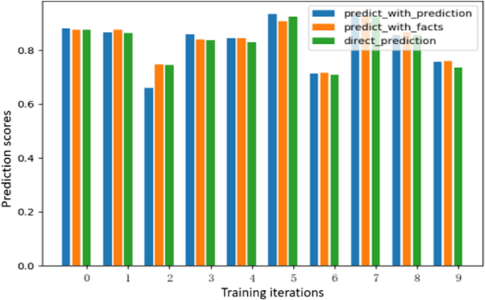
Predicted yield displacement results based on the three methods
The analyses above reveal that the iterative prediction combination approach can enhance the accuracy considerably. In addition, this study has explored the relationships among other mechanical performance parameters, such as the relationship between the ultimate load and the ultimate displacement, the relationship between the ultimate load and the yield load, and the relationship between the yield displacement and the ultimate displacement. However, the predictive results for these relationships are not ideal; and in some cases, the scores appear lower.
-
-
(2)
To predict target variables based on multivariate design of independent variables
The above design process mainly involves iterative predictions with two related variables. In practical models, however, multiple variables shall be considered to explore their relationships. Attempts were made in this study to predict the yield displacement based on the predicted elastic stiffness and the yield load.
Experimental results indicate that to fit the experimental data in combination with the predictions did not lead to an improvement, but may even result in a slight decline. The scores of twenty sets of model-training data are visualized in Fig. 6.
Fig. 6 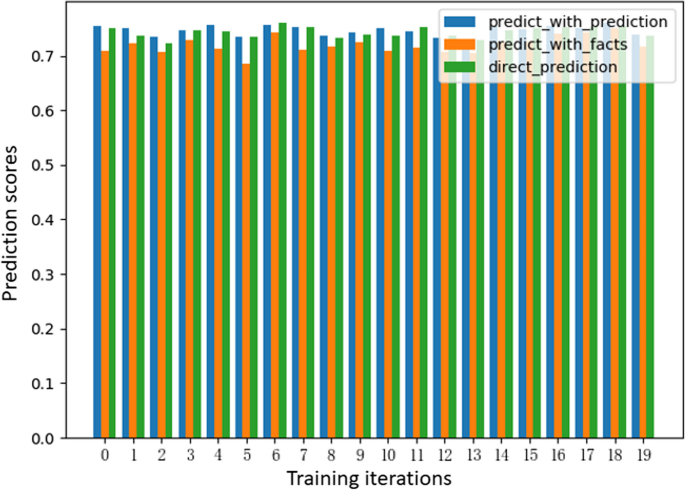
Comparison of prediction scores for each method
The training results mentioned above manifest that the most effective analysis method is to analyze experimental data individually. And the best approach is to focus on the relationship between design parameters and mechanical parameters, without delving into the interdependencies among the mechanical parameters. In other words, the approach of combining multiple single-variable predictions multiple times appears to be the most suitable.


3.2.3 Generalized overall model
In fact, multivariate output is also a model’s generalization capability. To achieve predictions from multiple input features for multiple target variables, a model accomplishing such functionality can be directly constructed. In this case, a Decision Tree model is used for constructing a multi-output model. The results of ten sets of model training are visualized in Fig. 7.

Comparison of prediction scores for different deep_max parameters
The deep_max parameter is a hyperparameter in the DT model. The larger the parameter, the better the model performs on the training data. When deep_max is adaptive, the scores are very close to 1. When this parameter is set to 2, the scores would be very low. The comparison of the above scores clearly indicates that the models with higher training depths have stronger generalization capabilities, resulting in more meaningful accuracy in prediction. There is a noticeable change when the training depth is shifted from 2 to 5 layers, but the training time exhibits an exponential growth from 0.08 s to 0.64 s.
3.2.4 Comparison
The comparison of the three approaches reveals that direct prediction of single variables is most adoptable. The iterative prediction of single variables performed better than direct prediction of single variables only in individual cases. The generalized overall model can produce more accurate predictions, but in the case of a large database, the training cost involved would increase rapidly.
4 The forward prediction model based on an augmented dataset
In this section, the original dataset is expanded within a certain range, and the boundary range of the braces’ force performance is analyzed based on the given design parameter range.
4.1 The expanded dataset
For the convenience of data analysis and representation of analytical methods, this section will investigate the relationship between parameters η and γ, while keeping length a and thickness t constant.
Expanding the existing dataset is crucial now for improving the model’s generalization ability, especially given the limited available data. Additionally, it’s worth noting that the dataset exhibits a continuous nature, particularly in the context of mechanical properties. This continuity is essential, as it underscores the importance of obtaining a more comprehensive dataset to capture the underlying regularities both in the input and output sets. In this study, two scenarios were analyzed: (1) Side length a = 150 mm, and plate thickness t = 12 mm; and (2) a = 180 mm, and t = 13 mm. Then, the other two parameters were expanded in terms of their range and granularity. Initially, the range of crease-weakening coefficient η was extended from the original data set [0.4, 1] to a new set [0.2, 1], and the range of angle γ was from set [55°, 65°] to [50°, 70°]. Additionally, the granularity of data selection was increased: the step size for selecting crease-weakening coefficient η was reduced from 5 to 0.2, thus increasing the data selection granularity by a factor of 25. The step size for selecting angle γ was reduced from 0.2 to 0.02, thus increasing the data selection granularity by a factor of 10.
The expanded parameter dataset was used as an independent variable set for testing, and the experimental data were used as the training dataset for the DT model, in order to predict the key parameters of the origami brace’s mechanical performance.
4.2 Prediction of mechanical performance under different parameters
The above data analysis sets were imported into MATLAB for further analysis. A three-dimensional model was designed in high-order linear fitting methods. The model’s accuracy was adjusted by modifying different parameters. When the model reached a good level of accuracy without excessive complexity, it was represented in contour heat maps, with color variations indicating the magnitude of the third-dimensional data.
When the parallelogram section side’s length a is 150 mm and the plate thickness t is 12 mm, the corresponding actual data points from the original dataset could also be identified. In this context, the original data are presented in a rhombus shape on the corresponding contour heat map.
Figure 8 depicts the impact of crease-weakening coefficient η and angle γ on the elastic stiffness. As observed from the figure, an increase in η and γ leads to higher elastic stiffness. When η and γ are relatively small, the growth rate will become slower. Compared to Fig. 8(a), the changes shown in Fig. 8(b) are not pronounced, meaning that lower elastic stiffness will come with a higher maximum value.

Investigating the impact of η and γ on elastic stiffness
Figure 9 illustrates the impact of crease-weakening coefficient η and angle γ on the yield displacement. As showed in Fig. 9(a), when the angle γ increases, the yield displacement will show a trend of decreasing first and increasing later, with the peak value appearing approximately at the angle of 67°. When the angle remains constant, the yield displacement will not change very significantly with variations in the crease-weakening coefficient η.

Investigating the impact of η and γ on yield displacement
Figure 9(a) and (b) exhibit completely different characteristics. Figure 9(b) indicates that as the angle increases and the crease-weakening coefficient decreases, the yield displacement would gradually decrease. Additionally, the yield displacement is generally larger in Fig. 9(b).
The impacts of crease-weakening coefficient η and angle γ on the elastic stiffness and the yield load are similar. As presented in Fig. 10(a), the yield load’s behavior aligns well with the actual mechanical loading pattern. However, there’s a slight dip in the yield load when crease-weakening coefficient η reaches extremely high values and angle γ is relatively low.

Investigating the impact of η and γ on yield load
Figure 10(a) and (b) display similar trends. However, the data variation appears to be more structured and hierarchical in Fig. 10(b). The data transitions appear more pronounced.
Contrary to the case with the yield displacement, changes of angle γ show almost no effect on the ultimate load, while the increase of crease-weakening coefficient η leads to a decrease in the ultimate displacement. The law shown in Fig. 11(a) is similar to that in Fig. 11(b); however, with changes of angle γ, there is a slight fluctuation in the size of the limit displacement.

Investigating the impact of η and γ on ultimate displacement
As evident in Fig. 12(a), a clear hierarchical relationship exists with changes of the ultimate load, but there are errors within a certain range. The parts that do not conform to the change law are mainly concentrated in the areas beyond the actual original dataset, such as the areas with crease-weakening coefficient η below 0.4 and the included angle γ below 55°.

Investigating the impact of η and γ on ultimate load
Compared with Fig. 12(a), the hierarchical relationship is more obvious in Fig. 12(b), and there is an identity with the changes of crease-weakening coefficient η and angle γ. In other words, the ultimate load would increase with the increase of crease-weakening coefficient η, while decreasing with the increase of angle γ. In general, the change of the ultimate load is basically consistent with the stress law of the origami-inspired braces.
4.3 Analysis of the performance limits
In order to optimize the structural performance, a parameter set was identified within the specified independent variable ranges, so as to maximize the elastic stiffness, the yield load and the ultimate load, while minimizing the yield and ultimate displacement.
To some extent, the initial data analysis reveals that the structural performance demonstrates some synergy: the optimal states for all performance indicators coincide with each other. In other words, as the elastic stiffness increases, it will lead to a higher yield and ultimate load, while minimizing the yield and ultimate displacement. These changes are exactly what the structural design expects.
In this section, a Decision Tree model and an expanded dataset are utilized to obtain a robust model, aiming to find out the optimal structural performance within the specified range. The testing scheme covers a range of design parameters, with a cross-sectional side length between 170 mm and 180 mm, an angle between 60.2° and 64.2°, plate thickness between 8.4 mm and 10.4 mm, and a weakening factor between 0.62 and 0.82. After training the model with this extended and densely-gridded dataset, the predicted results were obtained. The results for the specific parameter values and mechanical properties are listed in Table 5.
5 Validation of the reverse prediction model and finite element analysis
The previous section determined the mechanical performance limits of the origami-inspired braces within specified parameter ranges. This section will establish a reverse prediction model to design the geometric parameters of the origami-inspired braces based on the given mechanical performance. Subsequently, the finite element analysis (FEA) will be conducted to validate two sets of geometric parameters designed by using the reverse prediction model.
5.1 Reverse prediction model
Based on the expanded dataset, a reverse prediction model was developed with the DT model by reversing the roles of input and output variables in Table 5. Two sets of data were chosen for validation: one with a descending portion, where the ultimate displacement is less than 50 mm; and the other without any descending portion, but with an ultimate displacement of 50 mm. The reverse prediction model was trained to predict the corresponding parameter designs. The score of the reverse training model was roughly 0.932. The final selected data is shown in Table 6.
5.2 Finite element verification
-
(1)
Model design
The designed brace component has a total length of 3000 mm and is composed of fifteen identical typical elements, each of which has a length L of 200 mm. To reduce the impact of eccentricity on the component, 1/4 of the typical elements near the braces are replaced with straight pipes, as shown in Fig. 13. The cross-sectional material is Q235 steel, and a bilinear material model is used. The model elements are all S4R elements.
Fig. 13 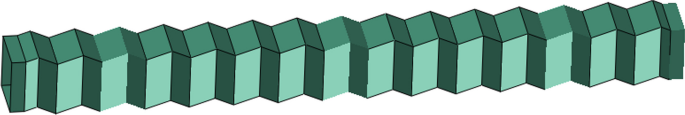
Schematic of the tubular components
-
(2)
Simulation results
To enhance clarity, the displacement display is magnified by a factor of 10. Figure 14 illustrates the variation in displacement during loading. The findings reveal that the structural deformation primarily involves axial compression, displaying a relatively uniform deformation process. Notably, the displacement is more pronounced near the load end, as highlighted in red, while the deformation near the fixed end, as depicted in blue, is comparatively minimal.
Fig. 14 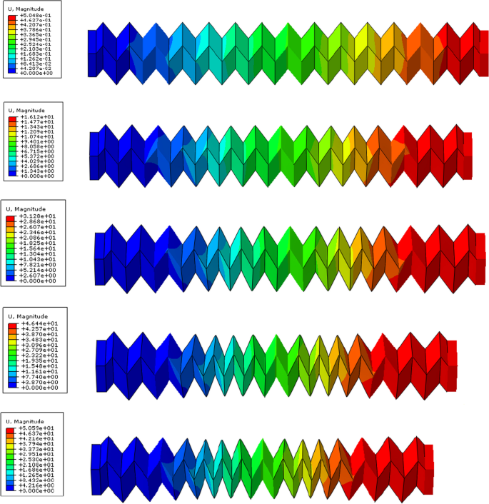
Deformation process of the origami-inspired braces
The chart of stress evolution clouds during the compression process of the support is illustrated in Fig. 15. The results indicate that the stress initially intensifies at the fold and subsequently diffuses gradually towards the center of the planar quadrilateral plate.
Fig. 15 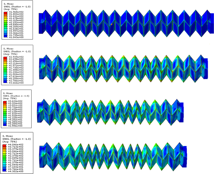
Stress evolution process of the origami-inspired braces
-
(3)
Comparison of the mechanical performance parameters
The load-displacement curve for Data Group 1 corresponding to the origami brace loading process was extracted, as shown in Fig. 16(a). During the 50 mm displacement loading process, the load consistently showed a monotonic increase, without any descending segments. As for the load-displacement curve for Data Group 2, as shown in Fig. 16(b), the load would first increase and then decrease with the increase of compression displacement. The model of the load-displacement curve is consistent with the design results. In addition, the errors of mechanical property parameters meet the design requirements, as presented in Table 7.
Fig. 16 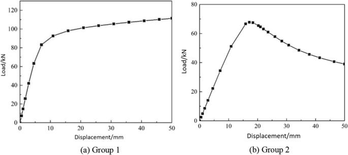
The load-displacement curve
Table 7 Results of finite element analysis for the origami-inspired braces It’s evident that the reverse prediction of the yield load and the ultimate displacement has yielded good results, and the maximum error is only 5.47%. In contrast, the error in the prediction of the elastic stiffness and ultimate load fluctuates from 7.26% to 16.73%. Among the above prediction targets, the absolute error fluctuation of the yield displacement is the smallest. In summary, the prediction model of this study delivers good results, but only two supporting data points are provided.


6 Conclusion
This study mainly explored the forward prediction of the mechanical performance of origami braces as well as the reverse prediction of their geometric parameters based on machine learning models, followed by finite element validation. Several machine learning methods were compared to analyze the mechanical performance of origami braces. The results show that the Decision Tree model has high accuracy and low training time.
Multiple approaches were taken to build multiple-input and multiple-output prediction models, including single performance prediction, multi-performance prediction, and generalized overall model. It is found that the most reasonable approach is to use multiple predictions of single variables. Taking into account the relationships between dependent variables for iterative combinations could lead to a decrease in accuracy. The generalized holistic model can achieve a certain level of accuracy, but the cost will grow exponentially in terms of training time.
Additionally, more fine-grained predictions and analyses were made by expanding the dataset within reasonable ranges of feature variables. Then an optimal set of parameters was determined. Finally, two groups of data were chosen to establish reverse prediction models, which were validated with finite element analysis results.
This study constructed certain design models for geometric parameters and mechanical performance of origami braces. However, the lack of static test data of origami braces is its limitation. In the future research, predictions will be verified in static tests.
Availability of data and materials
The data has been provided in Appendix.
References
Alaçam, S., Karadag, I., & Güzelci, O. Z. (2022). Reciprocal style and information transfer between historical Istanbul Pervititch maps and satellite views using machine learning. Estoa, Revista de la Facultad de Arquitectura y Urbanismo de la Universidad de Cuenca, 11(22), 97–113. https://doi.org/10.18537/est.v011.n022.a06
Bertoldi, K., Vitelli, V., Christensen, J., & van Hecke, M. (2017). Flexible mechanical metamaterials. Nature Reviews Materials, 2(11), 17066.
Cai, J., Zhong, Q., Pan, L., et al. (2023a). Nonlinear wrap-folding of membranes with predefined creases and seams. International Journal of Non-Linear Mechanics, 156, 104519.
Cai, J., Zhong, Q., Zhang, X., et al. (2023b). Mobility and kinematic bifurcation analysis of origami plate structures. Journal of Mechanisms and Robotics, 15(6), 061015.
Cai, J. G., Zhang, Q., Feng, J., & Xu, Y. X. (2019). Modeling and kinematic path selection of retractable kirigami roof structures. Computer-Aided Civil and Infrastructure Engineering, 34(4), 352–363.
Cai, J. G., Zhou, Y., Wang, X. Y., Xu, Y. X., Feng, J., & Deng, X. W. (2018). Dynamic analysis of a cylindrical boom based on Miura origami. Steel & Composite Structures, 28(5), 607–615.
Cehula, J., & Průša, V. (2020). Computer modelling of origami-like structures made of light-activated shape memory polymers. International Journal of Engineering Science, 150, 103235.
Chalab, R., Yazdanpanah, O., & Dolatshahi, K. M. (2023). Nonmodel rapid seismic assessment of eccentrically braced frames incorporating masonry infills using machine learning techniques. Journal of Building Engineering, 79, 107784.
Chen, P.-Y., & Guan, X. (2023). A multi-source data-driven approach for evaluating the seismic response of non-ductile reinforced concrete moment frames. Engineering Structures, 278, 115452.
Chen, W. J., Tian, X. Y., Gao, R. J., & Liu, S. T. (2018). A low porosity perforated mechanical metamaterial with negative Poisson’s ratio and band gaps. Smart Materials and Structures, 27(11), 115010.
Fatehi, E., Sarvestani, H. Y., Ashrafi, B., & Akbarzadeh, A. H. (2021). Accelerated design of architectured ceramics with tunable thermal resistance via a hybrid machine learning and finite element approach. Materials & Design, 210, 1–13. https://doi.org/10.1016/j.matdes.2021.110056
Filipov, E. T., Paulino, G. H., & Tachi, T. (2019). Deployable sandwich surfaces with high out-of-plane stiffness. Journal of the Structural Engineering, 145(2), 04018244.
Güzelci, O. Z. (2022). A machine learning-based model to predict the cap geometry of Anatolian Seljuk Kümbets. Periodica Polytechnica Architecture, 53(3), 207–219. https://doi.org/10.3311/PPar.20112
Hamidia, M., Mansourdehghan, S., Asjodi, A. H., & Dolatshahi, K. M. (2022a). Machine learning-aided scenario-based seismic drift measurement for RC moment frames using visual features of surface damage. Measurement, 205, 112195.
Hamidia, M., Mansourdehghan, S., Asjodi, A. H., & Dolatshahi, K. M. (2022b). Machine learning-based seismic damage assessment of non-ductile RC beam-column joints using visual damage indices of surface crack patterns. Structures (pp. 2038–2050). Elsevier.
Hayakawa, K., & Ohsaki, M. (2019). Frame model for analysis and form generation of rigid origami for deployable roof structure. In Proceedings of IASS annual symposia.
Hu, B., Min, Y., Wang, C., Xu, Q., & Keleta, Y. (2022). Design, analysis and application of the double-stage yield buckling restrained brace. Journal of Building Engineering, 48, 103980.
Jiang, Q., Wang, H., Feng, Y., Chong, X., Huang, J., Wang, S., et al. (2022). Analysis and experimental testing of a self-centering controlled rocking wall with buckling-restrained braces at the base. Engineering Structures, 269, 114843.
Karadag, I., Güzelci, O. Z., & Alaçam, S. (2022). EDU-AI: A twofold machine learning model to support classroom layout generation. Construction Innovation. https://doi.org/10.1108/CI-02-2022-0034
Li, H., Li, J., & Farhangi, V. (2023). Determination of piers shear capacity using numerical analysis and machine learning for generalization to masonry large scale walls. Structures (pp. 443–466). Elsevier.
Li, G. Q., Sun, Y. Z., Jiang, J., Sun, F. F., & Ji, C. (2019). Experimental study on two-level yielding buckling-restrained braces. Journal of Constructional Steel Research, 159, 260–269.
Liu, J., Ou, H. F., Zeng, R., Zhou, J. X., Long, K., Wen, G. L., & Xie, Y. M. (2019). Fabrication, dynamic properties and multi-objective optimization of a metal origami tube with Miura sheets. Thin-Walled Structures, 144, 106352.
Liu, Y., Zhang, W., Zhang, F. H., Lan, X., Leng, J. S., Liu, S., Jia, X. Q., Cotton, C., Sun, B. Z., Gu, B. H., & Chou, T. W. (2018). Shape memory behavior and recovery force of 4D printed laminated miura-origami structures subjected to compressive loading. Composites Part b: Engineering, 153, 233–242.
Ma, J., & You, Z. (2013). Energy absorption of thin-walled square tubes with a pre-folded origami pattern part I: Geometry and numerical simulation. Journal of Applied Mechanics, 81(1), 011003.
Ma, J. Y., Hou, D. G., Chen, Y., & You, Z. (2016). Quasi-static axial crushing of thin-walled tubes with a kite-shape rigid origami pattern: Numerical simulation. Thin-Walled Structures, 100, 38–47.
Maher, M. L., Merrick, K., & Saunders, R. (2007). From passive to proactive design elements. Computer-aided architectural design futures (CAADFutures) (pp. 447–460). Springer. https://doi.org/10.1007/978-1-4020-6528-6_33
Miura, K. (1985). Method of packaging and deployment of large membranes in space. In Proc. 31st Cong. Int. astronautical Federation (No. 618, pp. 1–9).
Ouisse, M., Collet, M., & Scarpa, F. (2016). A piezo-shunted kirigami auxetic lattice for adaptive elastic wave filtering. Smart Materials and Structures, 25(11), 115016.
Shigemune, H., Maeda, S., Hara, Y., Hosoya, N., & Hashimoto, S. (2016). Origami robot: A self-folding paper robot with an electrothermal actuator created by printing. IEEE/ASME Transactions on Mechatronics, 21(6), 2749–2754.
Song, J., Chen, Y., & Lu, G. X. (2012). Axial crushing of thin-walled structures with origami patterns. Thin-Walled Structures, 54, 65–71.
Sun, J., Pan, P., & Wang, H. (2018). Development and experimental validation of an assembled steel double-stage yield buckling restrained brace. Journal of Constructional Steel Research, 145, 330–340.
Tachi, T. (2010). One-DOF cylindrical deployable structures with rigid quadrilateral panels. In Evolution and trends in design, analysis and construction of shell and spatial structures: Proceedings.
Tamke, M., Nicholas, P., & Zwierzycki, M. (2018). Machine learning for architectural design: Practices and infrastructure. International Journal of Architectural Computing, 16(2), 123–143. https://doi.org/10.1177/1478077118778580
Topuz, B., & Çakici, A. L. P. N. (2023). Machine learning in architecture. Automation in Construction, 154, 105012.
Uzun, C., & Çolakoglu, M. B. (2019). Architectural drawing recognition: A case study for training the learning algorithm with architectural plan and section drawing images. In Education-and-research-in-computer-aided-architectural-design-in-Europe (eCAADe), Porto, Portugal (pp. 29–34). https://doi.org/10.5151/proceedings-ecaadesigradi2019_171
Vasileiadis, V., Kostinakis, K., & Athanatopoulou, A. (2023). Story-wise assessment of seismic behavior and fragility analysis of R/C frames considering the effect of masonry infills. Soil Dynamics and Earthquake Engineering, 165, 107714.
Wang, Z., & Ma, L. (2021). Effect of thickness stretching on bending and free vibration behaviors of functionally graded graphene reinforced composite plates. Applied Sciences, 11(23), 11362.
Wang Z, Wang T, Ding Y, et al. (2022). A simple refined plate theory for the analysis of bending, buckling and free vibration of functionally graded porous plates reinforced by graphene platelets. Mechanics of Advanced Materials and Structures.
Wang, Z., Wang, T., Ding, Y., et al. (2023). Free vibration analysis of functionally graded porous plates based on a new generalized single-variable shear deformation plate theory. Archive of Applied Mechanics, 93(6), 2549–2564.
Wang, C.-L., Gao, Y., Cheng, X., Zeng, B., & Zhao, S. (2019). Experimental investigation on H-section buckling-restrained braces with partially restrained flange. Engineering Structures, 199, 109584.
Watanabe, A., Hitomi, Y., Saeki, E., Wada, A., & Fujimoto, M. (1988). Properties of brace encased in buckling-restraining concrete and steel tube. Proceedings of Ninth World Conference on Earthquake Engineering, 4, 719–724.
Wu, J.-R., & Di Sarno, L. (2023). A machine-learning method for deriving state-dependent fragility curves of existing steel moment frames with masonry infills. Engineering Structures, 276, 115345.
Wu, N. H., Dimopoulou, M., Hsieh, H. H., & Chatzakis, C. (2019). A digital system for AR fabrication of bamboo structures through the discrete digitization of bamboo. In Education-and-research-in-computer-aided-architectural-design-in-Europe (eCAADe) (pp. 20–22). https://doi.org/10.5151/proceedingsecaadesigradi2019_538
Yu, Z., Su, R. K. L., Chen, H., et al. (2023). Evaluations of J-integral of nuclear graphite combining experimental and numerical methods. Theoretical and Applied Fracture Mechanics, 128, 104142.
Zhang, Q., Pan, N., Meloni, M., Lu, D., Cai, J. G., & Feng, J. (2021). Reliability analysis of radially retractable roofs with revolute joint clearances. Reliability Engineering & System Safety, 208, 107401.
Zhang, X., Cheng, G. D., You, Z., & Zhang, H. (2007). Energy absorption of axially compressed thin-walled square tubes with patterns. Thin-Walled Structures, 45(9), 737–746.
Zhou, Y., Zhang, Q., Cai, J., et al. (2021). Experimental study of the hysteretic behavior of energy dissipation braces based on Miura origami. Thin-Walled Structures, 167, 108196.
Zhou, Y., Zhang, Q., Zhou, Y., et al. (2023a). Buckling-controlled braces for seismic resistance inspired by origami patterns. Engineering Structures, 294, 116771.
Zhou, Y., Zhang, Y., Feng, J., et al. (2023b). Numerical study of the hysteretic behavior of energy dissipation braces based on Miura origami. International Journal of Non-Linear Mechanics, 157, 104523.
Zhu, F., Lu, R., Bai, P., et al. (2019). A novel in situ calibration of object distance of an imaging lens based on optical refraction and two-dimensional DIC. Optics and Lasers in Engineering, 120, 110–117.
Zhu, F., Lu, R., Gu, J., et al. (2020). High-resolution and high-accuracy optical extensometer based on a reflective imaging technique. Optics and Lasers in Engineering, 132, 106–136.
Zhu, B. L., Guo, Y. L., & Zhou, P. (2017). Numerical and experimental studies of corrugated-web-connected buckling-restrained braces. Engineering Structures, 134, 107–124.
Zhuge, Y., Ma, X., & Zeng, J. (2022). Recent progress in buckling restrained braces: A review on material development and selection. Advances in Structural Engineering, 25(7), 1549–1564.
Acknowledgements
The research presented in the paper was supported by the Jiangsu Provincial Department of Science and Technology Projects (BZ2022049 and BE2023801).
Funding
The research presented in the paper was supported by the Jiangsu Provincial Department of Science and Technology Projects (BZ2022049 and BE2023801).
Author information
Authors and Affiliations
Contributions
Jianguo Cai: supervision, conceptualization, funding acquisition, investigation. Huafei Xu: methodology, validation, writing—original draft. Jiacheng Chen and Qian Zhang: writing—original draft, visualization. Jian Feng: funding acquisition.
Corresponding author
Ethics declarations
Competing interests
There are no financial and non-financial competing interests.
Additional information
Publisher's Note
Springer Nature remains neutral with regard to jurisdictional claims in published maps and institutional affiliations.
Appendix
Appendix
1.1 Raw-data
a (mm) | γ (°) | t (mm) | η | Ke (N/mm) | Δy (mm) | Py (kN) | Δmax (mm) | Pmax (kN) |
|---|---|---|---|---|---|---|---|---|
100 | 55 | 8 | 0.4 | 815 | 15.44 | 5.19 | 50 | 14.2 |
100 | 55 | 8 | 0.6 | 1814 | 11.18 | 18.75 | 20.8 | 24.53 |
100 | 55 | 8 | 0.8 | 2730 | 9.97 | 17.19 | 16 | 32.15 |
100 | 55 | 8 | 1 | 3413 | 9.67 | 21.47 | 15.1 | 39.19 |
100 | 55 | 10 | 0.4 | 1503 | 13 | 9.53 | 43.7 | 21.92 |
100 | 55 | 10 | 0.6 | 3254 | 9.25 | 20.33 | 17.7 | 35.85 |
100 | 55 | 10 | 0.8 | 4801 | 8.25 | 29.84 | 13.9 | 46.35 |
100 | 55 | 10 | 1 | 5925 | 8.02 | 36.83 | 13.1 | 56.02 |
100 | 55 | 12 | 0.4 | 2465 | 11.18 | 15.45 | 36.8 | 31.16 |
100 | 55 | 12 | 0.6 | 5204 | 7.92 | 31.81 | 15.8 | 48.89 |
100 | 55 | 12 | 0.8 | 7541 | 7.09 | 45.77 | 12.75 | 62.66 |
100 | 55 | 12 | 1 | 9203 | 7.01 | 56.01 | 11.95 | 75.12 |
100 | 55 | 14 | 0.4 | 3730 | 9.8 | 22.96 | 31.05 | 41.79 |
100 | 55 | 14 | 0.6 | 7686 | 6.98 | 45.65 | 14.5 | 63.57 |
100 | 55 | 14 | 0.8 | 10,956 | 6.37 | 64.5 | 11.9 | 80.93 |
100 | 55 | 14 | 1 | 13,239 | 6.28 | 78.22 | 11.15 | 96.43 |
100 | 55 | 16 | 0.4 | 5318 | 8.75 | 32 | 27.1 | 53.75 |
100 | 55 | 16 | 0.6 | 10,710 | 6.31 | 61.49 | 13.65 | 79.86 |
100 | 55 | 16 | 0.8 | 15,036 | 5.79 | 85.19 | 11.35 | 101.11 |
100 | 55 | 16 | 1 | 18,008 | 5.75 | 102.71 | 10.6 | 119.73 |
100 | 60 | 8 | 0.4 | 1729 | 10.48 | 10.81 | 50 | 19.85 |
100 | 60 | 8 | 0.6 | 3991 | 9.25 | 24.5 | 28.4 | 42.04 |
100 | 60 | 8 | 0.8 | 6150 | 8.21 | 38.16 | 14.5 | 62.19 |
100 | 60 | 8 | 1 | 7799 | 8.37 | 48.87 | 12.55 | 78.24 |
100 | 60 | 10 | 0.4 | 3204 | 8.89 | 19.26 | 50 | 31.36 |
100 | 60 | 10 | 0.6 | 7207 | 7.56 | 42.77 | 20 | 63.9 |
100 | 60 | 10 | 0.8 | 10,875 | 6.8 | 65.86 | 11.55 | 89.52 |
100 | 60 | 10 | 1 | 13,587 | 6.94 | 84.03 | 10.2 | 112.15 |
100 | 60 | 12 | 0.4 | 5277 | 7.81 | 30.59 | 50 | 45.57 |
100 | 60 | 12 | 0.6 | 11,576 | 6.4 | 66.2 | 15.1 | 88.81 |
100 | 60 | 12 | 0.8 | 17,126 | 6 | 101 | 9.9 | 121.3 |
100 | 60 | 12 | 1 | 21,119 | 6.24 | 128.35 | 9 | 148.66 |
100 | 60 | 14 | 0.4 | 8011 | 7.05 | 44.68 | 50 | 62.27 |
100 | 60 | 14 | 0.6 | 17,140 | 5.59 | 93.54 | 12.6 | 116.44 |
100 | 60 | 14 | 0.8 | 24,888 | 5.34 | 140.61 | 8.8 | 155.38 |
100 | 60 | 14 | 1 | 30,327 | 5.51 | 176.01 | 8.1 | 189.42 |
100 | 60 | 16 | 0.4 | 11,450 | 6.44 | 60.99 | 46.15 | 81.18 |
100 | 60 | 16 | 0.6 | 23,898 | 5.03 | 125.01 | 11.05 | 146.72 |
100 | 60 | 16 | 0.8 | 34,091 | 4.85 | 182.69 | 8.1 | 192.75 |
100 | 60 | 16 | 1 | 41,093 | 5.11 | 226.64 | 7.55 | 233.2 |
100 | 65 | 8 | 0.4 | 3539 | 7.28 | 20.11 | 50 | 27.31 |
100 | 65 | 8 | 0.6 | 8201 | 6.67 | 45.54 | 30.9 | 59.41 |
100 | 65 | 8 | 0.8 | 12,666 | 6.48 | 73.08 | 14.85 | 96.3 |
100 | 65 | 8 | 1 | 16,088 | 6.13 | 96.04 | 9.95 | 119.59 |
100 | 65 | 10 | 0.4 | 6513 | 6.2 | 34.56 | 50 | 43.31 |
100 | 65 | 10 | 0.6 | 14,638 | 5.68 | 75.72 | 22.95 | 91.75 |
100 | 65 | 10 | 0.8 | 22,033 | 5.09 | 119.95 | 9.4 | 135.12 |
100 | 65 | 10 | 1 | 27,485 | 5.32 | 157.72 | 8.15 | 170.72 |
100 | 65 | 12 | 0.4 | 10,649 | 5.47 | 52.38 | 50 | 63.21 |
100 | 65 | 12 | 0.6 | 23,208 | 4.79 | 112.52 | 13.75 | 128.24 |
100 | 65 | 12 | 0.8 | 34,097 | 4.53 | 174.45 | 8 | 182.34 |
100 | 65 | 12 | 1 | 41,869 | 4.72 | 220.53 | 7.35 | 225.86 |
100 | 65 | 14 | 0.4 | 16,035 | 4.96 | 73.6 | 50 | 87.05 |
100 | 65 | 14 | 0.6 | 33,881 | 4.24 | 155.24 | 10.9 | 169.68 |
100 | 65 | 14 | 0.8 | 48,662 | 4.14 | 231.67 | 7.15 | 234 |
100 | 65 | 14 | 1 | 58,918 | 4.37 | 288.77 | 6.5 | 288.86 |
100 | 65 | 16 | 0.4 | 22,718 | 4.56 | 97.99 | 43.65 | 113.32 |
100 | 65 | 16 | 0.6 | 46,552 | 3.86 | 202.6 | 9.35 | 214.34 |
100 | 65 | 16 | 0.8 | 65,460 | 3.81 | 289.29 | 6.55 | 289.44 |
100 | 65 | 16 | 1 | 78,261 | 4.07 | 352.39 | 6.1 | 353.27 |
125 | 55 | 8 | 0.4 | 931 | 15.11 | 5.93 | 50 | 15.99 |
125 | 55 | 8 | 0.6 | 2066 | 14.56 | 13.15 | 50 | 35.09 |
125 | 55 | 8 | 0.8 | 3080 | 14.52 | 19.59 | 30.45 | 55.17 |
125 | 55 | 8 | 1 | 3816 | 14.54 | 24.25 | 24.25 | 70.23 |
125 | 55 | 10 | 0.4 | 1733 | 12.82 | 11.03 | 50 | 25.27 |
125 | 55 | 10 | 0.6 | 3768 | 12.58 | 23.85 | 50 | 55.22 |
125 | 55 | 10 | 0.8 | 5532 | 11.64 | 35.11 | 22.6 | 80.44 |
125 | 55 | 10 | 1 | 6779 | 12.23 | 43.05 | 19.1 | 100.4 |
125 | 55 | 12 | 0.4 | 2871 | 11.23 | 18.05 | 50 | 36.79 |
125 | 55 | 12 | 0.6 | 6127 | 10.8 | 38.18 | 38.2 | 77.48 |
125 | 55 | 12 | 0.8 | 8870 | 10.02 | 55.97 | 18.65 | 108.64 |
125 | 55 | 12 | 1 | 10,769 | 10.54 | 68.25 | 16.15 | 134.38 |
125 | 55 | 14 | 0.4 | 4388 | 10.05 | 27.04 | 50 | 50.59 |
125 | 55 | 14 | 0.6 | 9199 | 9.36 | 56.27 | 29.65 | 102.66 |
125 | 55 | 14 | 0.8 | 13,147 | 8.88 | 82.1 | 16.35 | 140.85 |
125 | 55 | 14 | 1 | 15,832 | 9.43 | 100.09 | 14.2 | 172.46 |
125 | 55 | 16 | 0.4 | 6320 | 9.14 | 38.09 | 50 | 66.72 |
125 | 55 | 16 | 0.6 | 13,024 | 8.33 | 78.15 | 24.75 | 130.73 |
125 | 55 | 16 | 0.8 | 18,389 | 7.96 | 113.44 | 14.6 | 175.87 |
125 | 55 | 16 | 1 | 21,978 | 8.46 | 138.33 | 12.85 | 213.31 |
125 | 60 | 8 | 0.4 | 1944 | 10.36 | 12.14 | 50 | 22.03 |
125 | 60 | 8 | 0.6 | 4436 | 9.89 | 27.31 | 50 | 49.33 |
125 | 60 | 8 | 0.8 | 6748 | 10.88 | 42.11 | 39.3 | 82.71 |
125 | 60 | 8 | 1 | 8470 | 11 | 53.31 | 23.75 | 114.78 |
125 | 60 | 10 | 0.4 | 3619 | 8.75 | 21.73 | 50 | 34.89 |
125 | 60 | 10 | 0.6 | 8084 | 8.51 | 48.27 | 50 | 78.32 |
125 | 60 | 10 | 0.8 | 12,073 | 8.59 | 73.85 | 21.4 | 122.81 |
125 | 60 | 10 | 1 | 14,950 | 8.82 | 93.45 | 15.95 | 161.25 |
125 | 60 | 12 | 0.4 | 5991 | 7.64 | 34.67 | 50 | 50.94 |
125 | 60 | 12 | 0.6 | 13,110 | 7.56 | 75.38 | 43.85 | 111.75 |
125 | 60 | 12 | 0.8 | 19,250 | 7.31 | 115.41 | 16.45 | 170.37 |
125 | 60 | 12 | 1 | 23,559 | 7.65 | 145.41 | 13.3 | 219.14 |
125 | 60 | 14 | 0.4 | 9144 | 6.83 | 50.77 | 50 | 70.28 |
125 | 60 | 14 | 0.6 | 19,601 | 6.73 | 107.61 | 34.95 | 150.43 |
125 | 60 | 14 | 0.8 | 28,328 | 6.51 | 165.14 | 13.95 | 223.79 |
125 | 60 | 14 | 1 | 34,313 | 6.9 | 208.86 | 11.6 | 281.97 |
125 | 60 | 16 | 0.4 | 13,144 | 6.21 | 69.52 | 50 | 93.03 |
125 | 60 | 16 | 0.6 | 27,605 | 6.09 | 145.39 | 28.05 | 193.63 |
125 | 60 | 16 | 0.8 | 39,298 | 5.84 | 221.43 | 12.2 | 281.46 |
125 | 60 | 16 | 1 | 47,152 | 6.33 | 282.36 | 10.4 | 351.17 |
125 | 65 | 8 | 0.4 | 3953 | 7.2 | 22.44 | 50 | 30.33 |
125 | 65 | 8 | 0.6 | 9030 | 6.95 | 50.49 | 50 | 68.4 |
125 | 65 | 8 | 0.8 | 13,752 | 7.43 | 80.14 | 26.5 | 113.52 |
125 | 65 | 8 | 1 | 17,285 | 7.64 | 104.33 | 16.8 | 158.35 |
125 | 65 | 10 | 0.4 | 7295 | 6.12 | 38.66 | 50 | 48.29 |
125 | 65 | 10 | 0.6 | 16,226 | 6.07 | 84.78 | 50 | 108.58 |
125 | 65 | 10 | 0.8 | 24,145 | 6.33 | 134.35 | 19 | 172.91 |
125 | 65 | 10 | 1 | 29,846 | 6.53 | 175.62 | 13.15 | 235.25 |
125 | 65 | 12 | 0.4 | 11,971 | 5.38 | 58.71 | 50 | 70.89 |
125 | 65 | 12 | 0.6 | 25,923 | 5.44 | 126.93 | 42.1 | 156.08 |
125 | 65 | 12 | 0.8 | 37,764 | 5.58 | 200.31 | 15.2 | 242.64 |
125 | 65 | 12 | 1 | 46,025 | 5.82 | 263.25 | 10.95 | 320.53 |
125 | 65 | 14 | 0.4 | 18,099 | 4.84 | 82.41 | 50 | 98.31 |
125 | 65 | 14 | 0.6 | 38,167 | 4.93 | 176.11 | 32.8 | 209.98 |
125 | 65 | 14 | 0.8 | 54,514 | 4.9 | 278.17 | 11.15 | 317.38 |
125 | 65 | 14 | 1 | 65,618 | 5.19 | 363.16 | 9.1 | 407.23 |
125 | 65 | 16 | 0.4 | 25,763 | 4.44 | 109.83 | 50 | 130.75 |
125 | 65 | 16 | 0.6 | 52,920 | 4.55 | 231.88 | 26.35 | 269.82 |
125 | 65 | 16 | 0.8 | 74,204 | 4.51 | 364.24 | 9.85 | 398.34 |
125 | 65 | 16 | 1 | 88,331 | 4.88 | 474.15 | 8.25 | 503.14 |
150 | 55 | 8 | 0.4 | 1031 | 15 | 6.57 | 50 | 17.45 |
150 | 55 | 8 | 0.6 | 2266 | 14.7 | 14.43 | 50 | 38.44 |
150 | 55 | 8 | 0.8 | 3343 | 16.69 | 21.27 | 50 | 65.77 |
150 | 55 | 8 | 1 | 4106 | 17.45 | 26.11 | 36 | 89.75 |
150 | 55 | 10 | 0.4 | 1927 | 12.67 | 12.28 | 50 | 27.61 |
150 | 55 | 10 | 0.6 | 4162 | 12.55 | 26.42 | 50 | 61.02 |
150 | 55 | 10 | 0.8 | 6052 | 14.09 | 38.49 | 40.5 | 100.64 |
150 | 55 | 10 | 1 | 7359 | 14.35 | 46.79 | 27.1 | 131.73 |
150 | 55 | 12 | 0.4 | 3205 | 11.06 | 20.16 | 50 | 40.21 |
150 | 55 | 12 | 0.6 | 6812 | 11.08 | 42.59 | 50 | 89.2 |
150 | 55 | 12 | 0.8 | 9782 | 11.88 | 61.97 | 30.15 | 140.11 |
150 | 55 | 12 | 1 | 11,792 | 12.37 | 74.92 | 22.15 | 179.49 |
150 | 55 | 14 | 0.4 | 4919 | 9.86 | 30.29 | 50 | 55.33 |
150 | 55 | 14 | 0.6 | 10,293 | 9.98 | 63.27 | 50 | 123.03 |
150 | 55 | 14 | 0.8 | 14,611 | 10.31 | 91.85 | 24.2 | 184.41 |
150 | 55 | 14 | 1 | 17,481 | 10.93 | 110.9 | 18.95 | 232.44 |
150 | 55 | 16 | 0.4 | 7112 | 8.94 | 42.78 | 50 | 73.03 |
150 | 55 | 16 | 0.6 | 14,664 | 9.2 | 88.65 | 50 | 161.78 |
150 | 55 | 16 | 0.8 | 20,594 | 9.19 | 128.21 | 20.7 | 233.51 |
150 | 55 | 16 | 1 | 24,471 | 9.95 | 154.89 | 16.9 | 291.76 |
150 | 60 | 8 | 0.4 | 2147 | 10.29 | 13.42 | 50 | 24.14 |
150 | 60 | 8 | 0.6 | 4856 | 9.95 | 29.99 | 50 | 54.18 |
150 | 60 | 8 | 0.8 | 7321 | 11.29 | 45.79 | 50 | 94.12 |
150 | 60 | 8 | 1 | 9127 | 12.31 | 57.53 | 32.65 | 132.71 |
150 | 60 | 10 | 0.4 | 4005 | 8.68 | 24.04 | 50 | 38.26 |
150 | 60 | 10 | 0.6 | 8885 | 8.53 | 53.3 | 50 | 86.37 |
150 | 60 | 10 | 0.8 | 13,167 | 9.81 | 81 | 43.6 | 145.46 |
150 | 60 | 10 | 1 | 16,206 | 10.34 | 101.63 | 24.65 | 200.39 |
150 | 60 | 12 | 0.4 | 6646 | 7.56 | 38.46 | 50 | 55.92 |
150 | 60 | 12 | 0.6 | 14,468 | 7.56 | 83.73 | 50 | 126.65 |
150 | 60 | 12 | 0.8 | 21,109 | 8.57 | 127.59 | 33.35 | 205.24 |
150 | 60 | 12 | 1 | 25,697 | 8.74 | 159.61 | 18.05 | 272.93 |
150 | 60 | 14 | 0.4 | 10,167 | 6.74 | 56.43 | 50 | 77.23 |
150 | 60 | 14 | 0.6 | 21,728 | 6.85 | 120.2 | 50 | 175.19 |
150 | 60 | 14 | 0.8 | 31,245 | 7.47 | 184.66 | 22.75 | 271.18 |
150 | 60 | 14 | 1 | 37,668 | 7.84 | 231.34 | 15.5 | 357.41 |
150 | 60 | 16 | 0.4 | 14,650 | 6.12 | 77.43 | 50 | 102.29 |
150 | 60 | 16 | 0.6 | 30,743 | 6.35 | 163.21 | 50 | 231.47 |
150 | 60 | 16 | 0.8 | 43,605 | 6.75 | 249.83 | 19 | 346.19 |
150 | 60 | 16 | 1 | 52,112 | 7.19 | 315.93 | 13.75 | 449.07 |
150 | 65 | 8 | 0.4 | 4363 | 7.13 | 24.72 | 50 | 33.3 |
150 | 65 | 8 | 0.6 | 9868 | 6.96 | 55.38 | 50 | 75.35 |
150 | 65 | 8 | 0.8 | 14,904 | 7.85 | 87.3 | 39.75 | 128.96 |
150 | 65 | 8 | 1 | 18,618 | 8.22 | 112.72 | 20.85 | 181.13 |
150 | 65 | 10 | 0.4 | 8062 | 6.06 | 42.67 | 50 | 53.09 |
150 | 65 | 10 | 0.6 | 17,791 | 6.04 | 93.6 | 50 | 120.85 |
150 | 65 | 10 | 0.8 | 26,296 | 6.77 | 147.86 | 28.95 | 198.82 |
150 | 65 | 10 | 1 | 32,333 | 7.03 | 191.5 | 15.8 | 271.85 |
150 | 65 | 12 | 0.4 | 13,250 | 5.32 | 64.75 | 50 | 78.01 |
150 | 65 | 12 | 0.6 | 28,536 | 5.43 | 140.41 | 50 | 178.09 |
150 | 65 | 12 | 0.8 | 41,357 | 6 | 222.61 | 21.85 | 280.79 |
150 | 65 | 12 | 1 | 50,179 | 6.24 | 289.61 | 13 | 375.35 |
150 | 65 | 14 | 0.4 | 20,072 | 4.78 | 90.88 | 50 | 108.3 |
150 | 65 | 14 | 0.6 | 42,203 | 5 | 195.33 | 50 | 246.78 |
150 | 65 | 14 | 0.8 | 60,070 | 5.43 | 310.03 | 17.4 | 373.25 |
150 | 65 | 14 | 1 | 71,977 | 5.71 | 404.12 | 11.4 | 484.73 |
150 | 65 | 16 | 0.4 | 28,636 | 4.38 | 121.1 | 50 | 144.17 |
150 | 65 | 16 | 0.6 | 58,804 | 4.7 | 257.99 | 46.6 | 322.19 |
150 | 65 | 16 | 0.8 | 82,223 | 4.94 | 408.06 | 13.55 | 468.34 |
150 | 65 | 16 | 1 | 97,609 | 5.31 | 533.16 | 10.3 | 606.92 |
175 | 55 | 8 | 0.4 | 1139 | 14.84 | 7.26 | 50 | 19.05 |
175 | 55 | 8 | 0.6 | 2481 | 14.74 | 15.8 | 50 | 42.13 |
175 | 55 | 8 | 0.8 | 3627 | 16.93 | 23.09 | 50 | 72.44 |
175 | 55 | 8 | 1 | 4430 | 19.56 | 28.18 | 50 | 106.35 |
175 | 55 | 10 | 0.4 | 2133 | 12.53 | 13.59 | 50 | 30.13 |
175 | 55 | 10 | 0.6 | 4571 | 12.57 | 29.03 | 50 | 66.93 |
175 | 55 | 10 | 0.8 | 6596 | 14.65 | 41.98 | 50 | 114.88 |
175 | 55 | 10 | 1 | 7977 | 16.82 | 50.75 | 42.05 | 162.01 |
175 | 55 | 12 | 0.4 | 3555 | 10.92 | 22.35 | 50 | 43.9 |
175 | 55 | 12 | 0.6 | 7507 | 11.07 | 47.01 | 50 | 97.88 |
175 | 55 | 12 | 0.8 | 10,706 | 13.04 | 67.92 | 50 | 167.35 |
175 | 55 | 12 | 1 | 12,841 | 14.26 | 81.68 | 32.2 | 224.25 |
175 | 55 | 14 | 0.4 | 5465 | 9.71 | 33.57 | 50 | 60.44 |
175 | 55 | 14 | 0.6 | 11,381 | 9.93 | 70.16 | 50 | 135.22 |
175 | 55 | 14 | 0.8 | 16,059 | 11.79 | 101.24 | 44.35 | 224.16 |
175 | 55 | 14 | 1 | 19,123 | 12.54 | 121.49 | 26.55 | 293.78 |
175 | 55 | 16 | 0.4 | 7917 | 8.79 | 47.52 | 50 | 79.81 |
175 | 55 | 16 | 0.6 | 16,270 | 9.09 | 98.61 | 50 | 179.09 |
175 | 55 | 16 | 0.8 | 22,730 | 10.55 | 142.07 | 35.9 | 285.91 |
175 | 55 | 16 | 1 | 26,891 | 11.25 | 170.64 | 22.8 | 369.79 |
175 | 60 | 8 | 0.4 | 2394 | 10.12 | 14.93 | 50 | 26.44 |
175 | 60 | 8 | 0.6 | 5364 | 9.91 | 33.17 | 50 | 59.54 |
175 | 60 | 8 | 0.8 | 8023 | 11.33 | 50.22 | 50 | 104.35 |
175 | 60 | 8 | 1 | 9950 | 13.27 | 62.76 | 44.55 | 151.55 |
175 | 60 | 10 | 0.4 | 4464 | 8.54 | 26.72 | 50 | 41.92 |
175 | 60 | 10 | 0.6 | 9821 | 8.49 | 58.98 | 50 | 95.02 |
175 | 60 | 10 | 0.8 | 14,450 | 9.89 | 89.17 | 50 | 165.82 |
175 | 60 | 10 | 1 | 17,697 | 11.14 | 111.19 | 31.5 | 230.05 |
175 | 60 | 12 | 0.4 | 7409 | 7.43 | 42.75 | 50 | 61.29 |
175 | 60 | 12 | 0.6 | 16,014 | 7.51 | 92.78 | 50 | 139.6 |
175 | 60 | 12 | 0.8 | 23,215 | 8.96 | 140.62 | 50 | 239.15 |
175 | 60 | 12 | 1 | 28,133 | 9.71 | 175.24 | 24.85 | 321.45 |
175 | 60 | 14 | 0.4 | 11,340 | 6.63 | 62.68 | 50 | 84.68 |
175 | 60 | 14 | 0.6 | 24,092 | 6.79 | 133.78 | 50 | 193.64 |
175 | 60 | 14 | 0.8 | 34,450 | 8.05 | 204.08 | 40.1 | 322.88 |
175 | 60 | 14 | 1 | 41,364 | 8.69 | 255.04 | 20.85 | 428.87 |
175 | 60 | 16 | 0.4 | 16,352 | 6.01 | 85.96 | 50 | 112.22 |
175 | 60 | 16 | 0.6 | 34,157 | 6.25 | 181.82 | 50 | 257.5 |
175 | 60 | 16 | 0.8 | 48,219 | 7.34 | 278.48 | 32.9 | 414.16 |
175 | 60 | 16 | 1 | 57,421 | 7.9 | 350.06 | 17.8 | 541.44 |
175 | 65 | 8 | 0.4 | 4783 | 7.08 | 27.07 | 50 | 36.48 |
175 | 65 | 8 | 0.6 | 10,745 | 6.97 | 60.45 | 50 | 82.64 |
175 | 65 | 8 | 0.8 | 16,156 | 8.01 | 94.82 | 50 | 145.92 |
175 | 65 | 8 | 1 | 20,121 | 8.9 | 122.07 | 28.1 | 205.03 |
175 | 65 | 10 | 0.4 | 8838 | 6.03 | 46.74 | 50 | 58.21 |
175 | 65 | 10 | 0.6 | 19,402 | 6.05 | 102.56 | 50 | 132.84 |
175 | 65 | 10 | 0.8 | 28,579 | 7.12 | 161.35 | 47.65 | 230.12 |
175 | 65 | 10 | 1 | 35,054 | 7.6 | 208.54 | 20.15 | 310.96 |
175 | 65 | 12 | 0.4 | 14,528 | 5.29 | 70.85 | 50 | 85.59 |
175 | 65 | 12 | 0.6 | 31,180 | 5.42 | 154 | 50 | 196.39 |
175 | 65 | 12 | 0.8 | 45,086 | 6.35 | 244.4 | 36.25 | 327.04 |
175 | 65 | 12 | 1 | 54,601 | 6.77 | 317.4 | 16.6 | 434.88 |
175 | 65 | 14 | 0.4 | 22,022 | 4.75 | 99.46 | 50 | 118.91 |
175 | 65 | 14 | 0.6 | 46,223 | 4.96 | 214.48 | 50 | 273.95 |
175 | 65 | 14 | 0.8 | 65,716 | 5.79 | 341.78 | 28.45 | 436.76 |
175 | 65 | 14 | 1 | 78,717 | 6.29 | 448.06 | 15.3 | 582.22 |
175 | 65 | 16 | 0.4 | 31,445 | 4.35 | 132.62 | 50 | 158.41 |
175 | 65 | 16 | 0.6 | 64,581 | 4.63 | 283.93 | 50 | 365.93 |
175 | 65 | 16 | 0.8 | 90,391 | 5.37 | 452.84 | 23.8 | 562.08 |
175 | 65 | 16 | 1 | 107,232 | 5.84 | 593.54 | 13.5 | 733.48 |
200 | 55 | 8 | 0.4 | 1242 | 14.72 | 7.92 | 50 | 20.5 |
200 | 55 | 8 | 0.6 | 2691 | 14.76 | 17.14 | 50 | 45.44 |
200 | 55 | 8 | 0.8 | 3910 | 17.11 | 24.89 | 50 | 78.33 |
200 | 55 | 8 | 1 | 4751 | 19.73 | 30.23 | 50 | 115.01 |
200 | 55 | 10 | 0.4 | 2330 | 12.4 | 14.85 | 50 | 32.45 |
200 | 55 | 10 | 0.6 | 4971 | 12.56 | 31.59 | 50 | 72.23 |
200 | 55 | 10 | 0.8 | 7133 | 14.79 | 45.4 | 50 | 124.51 |
200 | 55 | 10 | 1 | 8587 | 17.59 | 54.65 | 50 | 180.89 |
200 | 55 | 12 | 0.4 | 3890 | 10.78 | 24.46 | 50 | 47.31 |
200 | 55 | 12 | 0.6 | 8184 | 11.04 | 51.37 | 50 | 105.72 |
200 | 55 | 12 | 0.8 | 11,612 | 13.12 | 73.71 | 50 | 182.17 |
200 | 55 | 12 | 1 | 13,869 | 15.39 | 88.23 | 41.15 | 254.46 |
200 | 55 | 14 | 0.4 | 5989 | 9.58 | 36.74 | 50 | 65.16 |
200 | 55 | 14 | 0.6 | 12,436 | 9.9 | 76.8 | 50 | 146.14 |
200 | 55 | 14 | 0.8 | 17,467 | 11.9 | 110.3 | 50 | 251.57 |
200 | 55 | 14 | 1 | 20,718 | 13.52 | 131.68 | 33.25 | 337.23 |
200 | 55 | 16 | 0.4 | 8688 | 8.66 | 52.06 | 50 | 86.08 |
200 | 55 | 16 | 0.6 | 17,816 | 9.04 | 108.23 | 50 | 193.73 |
200 | 55 | 16 | 0.8 | 24,786 | 11.09 | 155.32 | 50 | 329.01 |
200 | 55 | 16 | 1 | 29,220 | 12.12 | 185.5 | 28.2 | 429.6 |
200 | 60 | 8 | 0.4 | 2583 | 10.09 | 16.12 | 50 | 28.53 |
200 | 60 | 8 | 0.6 | 5763 | 9.95 | 35.68 | 50 | 64.21 |
200 | 60 | 8 | 0.8 | 8585 | 11.44 | 53.78 | 50 | 112.55 |
200 | 60 | 8 | 1 | 10,610 | 13.63 | 66.92 | 50 | 165 |
200 | 60 | 10 | 0.4 | 4824 | 8.51 | 28.88 | 50 | 45.3 |
200 | 60 | 10 | 0.6 | 10,581 | 8.51 | 63.63 | 50 | 102.56 |
200 | 60 | 10 | 0.8 | 15,521 | 9.95 | 95.94 | 50 | 179.75 |
200 | 60 | 10 | 1 | 18,955 | 11.66 | 119.02 | 37.85 | 252.82 |
200 | 60 | 12 | 0.4 | 8017 | 7.4 | 46.26 | 50 | 66.3 |
200 | 60 | 12 | 0.6 | 17,296 | 7.52 | 100.45 | 50 | 150.76 |
200 | 60 | 12 | 0.8 | 25,016 | 8.92 | 151.9 | 50 | 263.25 |
200 | 60 | 12 | 1 | 30,244 | 10.16 | 188.52 | 29.2 | 355.73 |
200 | 60 | 14 | 0.4 | 12,284 | 6.59 | 67.93 | 50 | 91.66 |
200 | 60 | 14 | 0.6 | 26,077 | 6.79 | 145.46 | 50 | 209.22 |
200 | 60 | 14 | 0.8 | 37,231 | 8.22 | 221.36 | 50 | 361.82 |
200 | 60 | 14 | 1 | 44,617 | 9.22 | 275.85 | 25.85 | 479.9 |
200 | 60 | 16 | 0.4 | 17,731 | 5.98 | 93.23 | 50 | 121.55 |
200 | 60 | 16 | 0.6 | 37,050 | 6.24 | 197.91 | 50 | 278.36 |
200 | 60 | 16 | 0.8 | 52,257 | 7.6 | 303.55 | 43.45 | 466.33 |
200 | 60 | 16 | 1 | 62,131 | 8.37 | 379.89 | 21.75 | 611.4 |
200 | 65 | 8 | 0.4 | 5141 | 7.12 | 29.12 | 50 | 39.61 |
200 | 65 | 8 | 0.6 | 11,524 | 7.02 | 65.07 | 50 | 89.22 |
200 | 65 | 8 | 0.8 | 17,327 | 8.07 | 101.96 | 50 | 157.88 |
200 | 65 | 8 | 1 | 21,574 | 9.23 | 130.93 | 33.55 | 224.25 |
200 | 65 | 10 | 0.4 | 9490 | 6.06 | 50.54 | 50 | 63.18 |
200 | 65 | 10 | 0.6 | 20,825 | 6.09 | 110.73 | 50 | 143.43 |
200 | 65 | 10 | 0.8 | 30,711 | 7.14 | 174.18 | 50 | 253.06 |
200 | 65 | 10 | 1 | 37,688 | 7.99 | 224.64 | 24.9 | 342.91 |
200 | 65 | 12 | 0.4 | 15,597 | 5.32 | 76.49 | 50 | 92.91 |
200 | 65 | 12 | 0.6 | 33,510 | 5.45 | 166.7 | 50 | 212.1 |
200 | 65 | 12 | 0.8 | 48,562 | 6.56 | 264.78 | 50 | 368.65 |
200 | 65 | 12 | 1 | 58,877 | 7.12 | 343.48 | 19.95 | 482.2 |
200 | 65 | 14 | 0.4 | 23,644 | 4.78 | 107.38 | 50 | 129.07 |
200 | 65 | 14 | 0.6 | 49,757 | 4.99 | 232.69 | 50 | 295.89 |
200 | 65 | 14 | 0.8 | 70,965 | 6 | 371.66 | 40.1 | 495.29 |
200 | 65 | 14 | 1 | 85,141 | 6.6 | 485.87 | 18.55 | 648.15 |
200 | 65 | 16 | 0.4 | 33,775 | 4.38 | 143.3 | 50 | 171.95 |
200 | 65 | 16 | 0.6 | 69,648 | 4.65 | 308.53 | 50 | 395.48 |
200 | 65 | 16 | 0.8 | 97,875 | 5.54 | 493.6 | 30.45 | 626.82 |
200 | 65 | 16 | 1 | 116,347 | 6.11 | 648.57 | 16.15 | 822.73 |
225 | 55 | 8 | 0.4 | 1355 | 14.55 | 8.64 | 50 | 22.08 |
225 | 55 | 8 | 0.6 | 2917 | 14.72 | 18.58 | 50 | 49.09 |
225 | 55 | 8 | 0.8 | 4215 | 17.2 | 26.83 | 50 | 84.84 |
225 | 55 | 8 | 1 | 5103 | 19.94 | 32.47 | 50 | 125.18 |
225 | 55 | 10 | 0.4 | 2545 | 12.25 | 16.22 | 50 | 34.96 |
225 | 55 | 10 | 0.6 | 5399 | 12.52 | 34.3 | 50 | 78.06 |
225 | 55 | 10 | 0.8 | 7707 | 14.85 | 49.05 | 50 | 134.97 |
225 | 55 | 10 | 1 | 9245 | 17.74 | 58.84 | 50 | 197.88 |
225 | 55 | 12 | 0.4 | 4251 | 10.65 | 26.69 | 50 | 50.99 |
225 | 55 | 12 | 0.6 | 8901 | 10.98 | 55.91 | 50 | 114.3 |
225 | 55 | 12 | 0.8 | 12,572 | 13.16 | 79.81 | 50 | 197.7 |
225 | 55 | 12 | 1 | 14,967 | 16.07 | 95.24 | 50 | 286.53 |
225 | 55 | 14 | 0.4 | 6549 | 9.45 | 40.09 | 50 | 70.25 |
225 | 55 | 14 | 0.6 | 13,545 | 9.84 | 83.7 | 50 | 158.07 |
225 | 55 | 14 | 0.8 | 18,948 | 11.91 | 119.72 | 50 | 273.47 |
225 | 55 | 14 | 1 | 22,407 | 14.44 | 142.46 | 43.05 | 382.7 |
225 | 55 | 16 | 0.4 | 9507 | 8.53 | 56.84 | 50 | 92.84 |
225 | 55 | 16 | 0.6 | 19,433 | 8.97 | 118.1 | 50 | 209.59 |
225 | 55 | 16 | 0.8 | 26,939 | 10.95 | 169.11 | 50 | 362.31 |
225 | 55 | 16 | 1 | 31,669 | 12.98 | 201.15 | 35.85 | 489.23 |
225 | 60 | 8 | 0.4 | 2824 | 9.95 | 17.57 | 50 | 30.84 |
225 | 60 | 8 | 0.6 | 6259 | 9.9 | 38.74 | 50 | 69.51 |
225 | 60 | 8 | 0.8 | 9276 | 11.46 | 58.12 | 50 | 122.19 |
225 | 60 | 8 | 1 | 11,421 | 13.69 | 72.05 | 50 | 181.36 |
225 | 60 | 10 | 0.4 | 5273 | 8.39 | 31.48 | 50 | 49.01 |
225 | 60 | 10 | 0.6 | 11,502 | 8.47 | 69.14 | 50 | 111.1 |
225 | 60 | 10 | 0.8 | 16,796 | 9.95 | 103.93 | 50 | 195.5 |
225 | 60 | 10 | 1 | 20,445 | 12.09 | 128.48 | 46.4 | 281.5 |
225 | 60 | 12 | 0.4 | 8762 | 7.3 | 50.44 | 50 | 71.75 |
225 | 60 | 12 | 0.6 | 18,817 | 7.47 | 109.24 | 50 | 163.44 |
225 | 60 | 12 | 0.8 | 27,114 | 8.89 | 164.77 | 50 | 287.41 |
225 | 60 | 12 | 1 | 32,688 | 10.59 | 204 | 35.8 | 397.03 |
225 | 60 | 14 | 0.4 | 13,427 | 6.51 | 74.02 | 50 | 99.25 |
225 | 60 | 14 | 0.6 | 28,401 | 6.74 | 158.53 | 50 | 226.99 |
225 | 60 | 14 | 0.8 | 40,422 | 8.12 | 240.65 | 50 | 397.99 |
225 | 60 | 14 | 1 | 48,322 | 9.7 | 299.06 | 33.7 | 540.56 |
225 | 60 | 16 | 0.4 | 19,386 | 11.88 | 119.01 | 50 | 131.68 |
225 | 60 | 16 | 0.6 | 40,398 | 12.74 | 262.55 | 50 | 302.19 |
225 | 60 | 16 | 0.8 | 56,835 | 15.41 | 446.91 | 50 | 526.01 |
225 | 60 | 16 | 1 | 67,432 | 15.18 | 640.73 | 24.8 | 675.81 |
225 | 65 | 8 | 0.4 | 5652 | 6.98 | 31.86 | 50 | 43.07 |
225 | 65 | 8 | 0.6 | 12,545 | 6.95 | 70.73 | 50 | 96.82 |
225 | 65 | 8 | 0.8 | 18,714 | 8.05 | 110.17 | 50 | 171.92 |
225 | 65 | 8 | 1 | 23,169 | 9.58 | 140.9 | 42.5 | 248.46 |
225 | 65 | 10 | 0.4 | 10,425 | 5.95 | 54.91 | 50 | 68.74 |
225 | 65 | 10 | 0.6 | 22,679 | 6.04 | 120.27 | 50 | 155.78 |
225 | 65 | 10 | 0.8 | 33,215 | 7.11 | 188.83 | 50 | 276.47 |
225 | 65 | 10 | 1 | 40,555 | 8.35 | 242.86 | 31.75 | 381.68 |
225 | 65 | 12 | 0.4 | 17,126 | 5.23 | 82.98 | 50 | 101.12 |
225 | 65 | 12 | 0.6 | 36,524 | 5.4 | 180.9 | 50 | 230.58 |
225 | 65 | 12 | 0.8 | 52,612 | 6.46 | 287.27 | 50 | 407.81 |
225 | 65 | 12 | 1 | 63,500 | 7.47 | 372.81 | 25.35 | 537.32 |
225 | 65 | 14 | 0.4 | 25,960 | 4.7 | 116.49 | 50 | 140.56 |
225 | 65 | 14 | 0.6 | 54,769 | 4.95 | 255.07 | 50 | 325.91 |
225 | 65 | 14 | 0.8 | 77,033 | 6.02 | 403.55 | 50 | 564.01 |
225 | 65 | 14 | 1 | 92,050 | 6.91 | 526.95 | 23.75 | 727.03 |
225 | 65 | 16 | 0.4 | 37,089 | 4.3 | 155.39 | 50 | 187.36 |
225 | 65 | 16 | 0.6 | 76,099 | 4.59 | 334.26 | 50 | 430.69 |
225 | 65 | 16 | 0.8 | 106,464 | 5.65 | 536.8 | 40.05 | 711.39 |
225 | 65 | 16 | 1 | 126,106 | 6.4 | 708.31 | 20.2 | 924.69 |
Rights and permissions
Open Access This article is licensed under a Creative Commons Attribution 4.0 International License, which permits use, sharing, adaptation, distribution and reproduction in any medium or format, as long as you give appropriate credit to the original author(s) and the source, provide a link to the Creative Commons licence, and indicate if changes were made. The images or other third party material in this article are included in the article's Creative Commons licence, unless indicated otherwise in a credit line to the material. If material is not included in the article's Creative Commons licence and your intended use is not permitted by statutory regulation or exceeds the permitted use, you will need to obtain permission directly from the copyright holder. To view a copy of this licence, visit http://creativecommons.org/licenses/by/4.0/.
About this article

Cite this article
Cai, J., Xu, H., Chen, J. et al. Prediction and design of mechanical properties of origami-inspired braces based on machine learning. AI Civ. Eng. 3, 3 (2024). https://doi.org/10.1007/s43503-024-00022-w
Received:
Revised:
Accepted:
Published:
DOI: https://doi.org/10.1007/s43503-024-00022-w