
Abstract
A substantial portion of global quantum computing research has been conducted using quantum mechanics, which recently has been applied to quantum computers. However, the design of a quantum algorithm requires a comprehensive understanding of quantum mechanics and physical procedures. This work presents a quantum procedure for estimating information gain. It is aimed at making quantum computing accessible to those without preliminary knowledge of quantum mechanics. The procedure can be a basis for building data mining processes according to measures from information theory using quantum computers. The main advantage of this procedure is the use of amplitude encoding and the inner product of two quantum states to calculate the conditional entropy between two vectors. The method was implemented using the IBM simulator and tested over a dataset of six features and a Boolean target variable. The results showed a correlation of 0.942 between the ranks achieved by the classical and quantum computations with a significance of p < 0.005.
1 Introduction and related work
Quantum computing (QC) stands out as a highly promising domain within computation, commanding a significant presence in global research efforts (Ying 2010). At its core, QC relies on the foundational principle of quantum physics, positing that electrons can simultaneously exhibit wave-like and particle-like properties (Robertson 1943). However, the development and maintenance of quantum computers include formidable challenges due to their vulnerability to noise and anomalies (Bennett et al. 1997; De Wolf 2019). Many technological firms have been involved in quantum computing and invested heavily in developing this industry (Zeng et al. 2017). Over the years, a broader view of the pros and cons of QC has emerged, and this discussion remains relevant in modern times (Boyer et al. 1998; De Wolf 2019).
Compared to classical computing, QC demonstrates the potential to reduce computational complexity, enabling extensive simultaneous processing, a concept well supported by research (Biamonte et al. 2017; Wiebe 2020). However, algorithms are not limited to classical or quantum computers; they can work together to achieve better results (Buffoni and Caruso 2021). Consequently, combining QC and classical computing has given rise to a growing discipline called Quantum Machine Learning (QML). The transformation of classical machine learning algorithms into quantum equivalents requires translating classical algorithmic logic into circuits composed of quantum gates (Benedetti et al. 2019; Alchieri et al. 2021). Recent studies have published various quantum algorithm applications, including learning the behavior of random variables (González et al. 2022; Pirhooshyaran and Terlaky 2021), the development of quantum convolutional networks for image learning (Hur et al. 2022; Tüysüz et al. 2021), the creation of generative adversarial networks (GANs) and transfer learning (Assouel et al. 2022; Azevedo et al. 2022; Zoufal et al. 2021), as well as the implementation of reinforcement learning (Dalla Pozza et al. 2022).
In physics, entropy plays a vital role in characterizing the uncertainty in the state of matter (Bein 2006). Due to the rapid development of information technology, entropy has gained importance in information theory in recent years. Consequently, considering the amount of data in events, random variables and probability, considerable information can be identified through distributions of data (Wehrl 1978). These information measures have significant applications in artificial intelligence and machine learning, such as constructing decision trees and optimizing classifier models (Kapur and Kesavan 1992). Additionally, entropy is an essential metric in data mining and machine learning that indicates model inconclusiveness or inaccuracy. Generally, low entropy indicates that valuable information can be easily extracted from the data, while high entropy indicates a more significant challenge to generate meaningful insights (Kaufmann et al. 2020; Kaufmann and Vecchio 2020; Liu et al. 2022).
When dealing with a wide variety of data types, calculating entropy using a quantum computer can be challenging. First, it is necessary to ensure that the input is encoded in such a way that it fits the constraints of quantum states. Second, a series of quantum gates must be constructed to approximate the input data's entropy. As quantum simulators are now becoming more widely available, methods have been developed to calculate the entropy of a random variable using quantum circuits. An example of such a method is the entropy “black box” that uses variable distribution to determine its amplitude encoding and estimate its entropy (Koren et al. 2023).
Decision trees are fundamental elements in machine learning, offering a flexible and easily comprehensible approach to decision-making and predictive tasks (Navada et al. 2011). Their hierarchical structure breaks down complex decision-making processes into simple, often binary, questions accessible to non-specialized individuals. Their ability to understand complex data relationships makes decision trees valuable and reliable for building predictive models (Ahmed and Kim 2017). Furthermore, understanding that a decision tree is not homogeneous is essential, as a series of internal nodes can generate different decision trees. The maximum number of trees that can be generated from given data is exponential (Charbuty and Abdulazeez 2021).
The Iterative Dichotomiser 3 (ID3) algorithm is a traditional method for constructing decision trees (Hssina et al. 2014; Jin et al. 2009). This method follows a divide-and-conquer strategy and uses information gain (IG) to assess the accuracy of the classification (Kent 1983). The value of the IG indicates the rate of entropy reduction and is calculated by the entropy of the distribution of the subtraction in the primary data structure. Consequently, higher IG values indicate a higher percentage of removed entropy (Batra and Agrawal 2018; Guleria et al. 2014). Thus, for each recursive iteration, the algorithm selects the highest IG feature and uses it to build the next step of the tree.
This work presents a quantum procedure for estimating IG in datasets with Boolean target variables. It is a generic procedure that can be applied to data mining processes. Section 2 describes the procedure's correctness and general implementation using quantum logic circuits. The motivation to carry out this research is expressed in two main aspects. The first refers to the accessibility of quantum computation for the data mining process without the need for prior physical knowledge. The second is the calculation of IG in QC as a basis for building decision tree models and other measures according to information theory. The proposed method's main advantage is the amplitude of its encoding and the inner product of two quantum states used to calculate the conditional entropy between two vectors. Section 3 presents a case study of a simple dataset that compares the proposed method with the classical computer method’s results. The results of the proposed method will then be compared using a dataset with six features, which will be presented in Section 4. Last, Section 5 will discuss the main conclusions and suggestions for future directions.
2 Quantum information gain
This section presents a new method for calculating quantum information gain for discrete value features and a Boolean target variable. The proposed method uses the Quantum Entropy “Black Box” (QEBB), which inputs a vector of occurrences and calculates the entropy using amplitude encoding and parameterized vectors (Koren et al. 2023). First, the procedure and its quantum logic will be described. Then, the implementation and correctness of the method will be presented. Table 1 presents the notations used in this study.
2.1 Quantum logic and gates
Let \(D\) be a dataset consisting of \(m\) features and \(n\) records, denoted as \(F=\left\{{F}_{1},\dots ,{F}_{m}\right\}\), and a target variable, denoted as \({Y}_{D}\). The method inputs \(D\) and a feature denoted as \(A\), such that \(A\in F\). At the beginning, the method uses the QEBB to calculate the entropy of \({Y}_{D}\), the initial entropy of the dataset, denoted as \(QH\left(D\right)\). The method consists of three sub-procedures, as follows:
-
1.
Classical computer preprocessing – Given \(A\in F\), the method iterates over distinct values in \(A\), denoted as \({D}_{E}\left(A\right)=\left\{{a}_{1},\dots ,{a}_{p}\right\}\), for \(p\le n\). For each \({a}_{i}\in {D}_{E}\left(A\right)\), the method stores \({Y}_{i}\), the target variable of records such that \(A={a}_{i}\). Let \(W=\{{w}_{1},\dots ,{w}_{p}\)} be a set of proportional parameters, such that each \({w}_{i}\) equals \(|{Y}_{i}|\) and represents the weight of \({a}_{i}\) in the dataset.
-
2.
Initialization of amplitude vectors – At this point, the method creates \({Q}_{h}\), a set of all QEBB(\({Y}_{i}\)). The algorithm transforms both \(W,{Q}_{h}\) to an amplitude encoding by concatenating all items into a single amplitude vector. Let \(\widetilde{W}, \widetilde{Q}\) be the amplitude vectors, such that \({\left|\widetilde{W}\right|}^{2}={\left|\widetilde{Q}\right|}^{2}=1\), satisfies:
$$\widetilde{W}=\frac{1}{\sqrt{\sum_{i=1}^{p}{w}_{i}}}\cdot \sum_{i=1}^{p}\sqrt{{w}_{i}}$$(1a)$$\widetilde{Q}=\frac{1}{\sqrt{\sum_{i=1}^{p}{q}_{i}}}\cdot \sum_{i=1}^{p}\sqrt{{q}_{i}}$$(2a)Thus, each \({w}_{i}\in W\) is converted to \(\frac{\sqrt{{w}_{i}}}{\sqrt{\sum_{i=1}^{p}{w}_{i}}}\) and each \({q}_{i}\in {Q}_{h}\) to \(\frac{\sqrt{{q}_{i}}}{\sqrt{\sum_{i=1}^{p}{q}_{i}}}\).
-
3.
Quantum operations and output – The proposed method creates two quantum circuits: first for W with \(\left\lfloor{\text{log}}_2\vert W\vert\right\rfloor+1\) qubit and second for \({Q}_{h}\) with \(\left\lfloor{\text{log}}_2\vert Q_h\vert\right\rfloor+1\) qubit. (1a), (2a) are set as the initial states, denoted as, \(|{\psi }_{w}\rangle\) and \(|{\psi }_{q}\rangle\), respectively. Next, the method applies the \(U\) gate with the parameters \(\theta =\frac{\pi }{2},\phi =0,\lambda =\pi\) for both circuits to move the states into superposition, which is equivalent to applying the Hadamard gate. The inner product of the states, denoted as \(\langle {\psi }_{w}|{\psi }_{q}\rangle\), can be used to measure the overlap between the state vectors \({\psi }_{w},{\psi }_{q}\). The probability of observing the system in the state \({\psi }_{w}\), given that it is in state \({\psi }_{q}\), can be calculated by \({\left|\langle {\psi }_{w}|{\psi }_{q}\rangle \right|}^{2}\). Thus, the inner product of both states describes the amount of conditional entropy achieved in the sub-dataset of feature \(A\). Subtracting \({\left|\langle {\psi }_{w}|{\psi }_{q}\rangle \right|}^{2}\) from the original entropy of the dataset, \(QH\left(D\right)\) yields the information gain achieved in dataset \(D\) by feature \(A\).
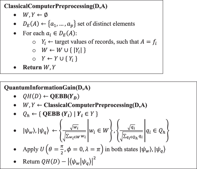

Table 2 provides the legend and description of the flow presented in Fig. 1

The quantum procedure flow of conditional entropy calculation
2.2 Correctness
Let \(D\) be a dataset consisting of \(m\) features and \(n\) records, denoted as \(F=\left\{{F}_{1},\dots ,{F}_{m}\right\}\), and a target variable, denoted as \({Y}_{D}\). Given \(A\in F\), let \({D}_{E}\left(A\right)=\left\{{a}_{1},\dots ,{a}_{p}\right\}\) be a set of distinct elements in feature \(A\), for \(p\le n\). For each value \({a}_{i}\in {D}_{E}\left(A\right)\), the method calculates \({w}_{i}\). The proportional parameter of \({a}_{i}\) equals \(|{Y}_{i}|\). Let \(W\) be a set of all \({w}_{i}\). Clearly,
The algorithm transforms \(W\) to an amplitude encoding by concatenating all items into a single amplitude vector. Let \((1a)\) be the amplitude vector, such that \({\left|\widetilde{W}\right|}^{2}=1\). The normalization constant, denoted as \(\widetilde{{W}_{c}}\), satisfies:
Each \({w}_{i}\in W\) is converted to \(\frac{\sqrt{{w}_{i}}}{\sqrt{\sum_{i=1}^{p}{w}_{i}}}\). Therefore, it satisfies the following:
Note that the same correctness holds for \((2a)\).
The Eq. (1a) is equivalent to (1b) as well as (2a) to (2b). The input vectors can be represented in the computational basis as \((1b)|i\rangle\) and \((2b)|i\rangle\). Since a quantum system of \(n\) qubits provide \({2}^{n}\) amplitudes, encoding \((1b),(2b)\) requires the use of \(\left\lfloor{\text{log}}_2\left|W\right|\right\rfloor+1\) qubit each, i.e., \(\left\lfloor{\text{log}}_2p\right\rfloor+1\). It is important to note that in cases where the length of \(\left(1b\right)\) or \((2b)\) is not to the power of two, zeros are added as their values do not change the IG calculation.
At this point, the method set the \(\left(1b\right), (2b)\) amplitude vectors as initial states, denoted as, \(|{\psi }_{w}\rangle\) and \(|{\psi }_{q}\rangle\), respectively. Since the normalization constant sums up to one, the coefficients of \(|{\psi }_{w}\rangle\) can describe the probability of each state, which is equivalent to the proportional parameter. Similarly, the coefficients of \(|{\psi }_{q}\rangle\) describe the relative entropy of each proportional parameter.
Next, the method creates two quantum circuits with \(2\left(\left\lfloor{\text{log}}_2p\right\rfloor+1\right)\) as the total number of qubits. By analyzing the worst case, all values in feature \(A\) are distinct, i.e., \(p=n\), and the total number of qubits equals twice the number needed for the complete dataset. Once the method allocates all qubits, it applies the \(U\) gate with the parameters \(\theta =\frac{\pi }{2},\phi =0,\lambda =\pi\) on both circuits independently, which moves the states into superposition. The following equations describe the quantum circuit over a single qubit, although the generalization to a higher dimension can be done with tensor products:
Let \(\langle {\psi }_{w}|{\psi }_{q}\rangle\) be the inner product of the states and let \({\left|\langle {\psi }_{w}|{\psi }_{q}\rangle \right|}^{2}\) be the probability of observing the system in the state \({\psi }_{w}\), given that it is in state \({\psi }_{q}\). The inner product can be understood as measuring the overlap between the state vectors \({\psi }_{w},{\psi }_{q}\). Since the value of \({\left|\langle {\psi }_{w}|{\psi }_{q}\rangle \right|}^{2}\) is a probability, it satisfies:
Thus, the inner product of these states:
Last, subtracting \({\left|\langle {\psi }_{w}|{\psi }_{q}\rangle \right|}^{2}\) from the original entropy of the dataset, \(QH\left(D\right)\), yields the IG achieved in dataset \(D\) by feature \(A\).
3 Case study
This section demonstrates a quantum IG calculation compared to classical computer computation. Table 3 presents a mockup dataset (\(D\)) consisting of feature \(A\) and a Boolean target variable, Y. First, the classic computer computation will be described, followed by the quantum procedure.
3.1 Classical computer computation
The IG is defined as the difference between the dataset entropy, \(H\left(Y\right)\), and the conditional entropy achieved by feature \(A\):
The initial entropy of the dataset can be calculated by:
The calculated conditional entropy is based on the probability distribution function of feature \(A\). For the demonstration, Table 4 presents the probability function, achieved by a simple preprocessing procedure.
The conditional entropy, \(H\left(Y|A\right)\), is defined as:
Last, the IG of dataset \(D\), achieved by feature \(A\), is:
3.2 Quantum computer computation
This section presents the case study and experiments of the IG calculation using the proposed method. The experiment was simulated using Qiskit (Cross 2018) and an IBM simulator with 1024 shots. To begin, the method used the QEBB (Koren et al. 2023) to obtain the initial entropy of the target variable.
Next, the method created and initialized W, the proportional parameter of each distinct value in \(A\), and \({Q}_{h}\), the vector of quantum entropy achieved by QEBB:
The quantum circuit converted \(W,{Q}_{h}\) into amplitude vectors. Applying the U gate and pushing the vectors into the superposition yielded state vectors of:
The inner product of both quantum states was defined as:
Last, the IG of dataset \(D\) achieved by feature \(A\) was:
The difference between the result obtained in classical computing and the proposed method is 0.045. For further analysis, see Section 4.
4 Results
This section compares and analyzes the proposed and classical computer computation methods for calculating IG. For the comparison, the diabetes dataset was used (Kahn 1994), which is a dataset of 768 diabetic and non-diabetic women. It consists of eight features and a Boolean target variable. Since the proposed method was designed for discrete values, the “BMI” and “DiabetesPedigreeFunction” features were removed.
Table 5 presents the six features of the dataset and compares the IG obtained in both classical computer calculation and quantum computation. The initial entropy was 0.933 for the classic calculation and 0.932 for the quantum computation. The minimal error obtained in the dataset appears in the glucose feature, with an error of 0.001, while the highest error was accrued in the skin thickness feature, with an error of 0.075.
Building a decision tree using the ID3 algorithm includes searching for the feature with the maximum IG value to be the root of the tree. In both methods, the glucose feature was chosen as the tree's root. Since the error of this feature was the minimal error achieved, it can be concluded that there was correspondence between the methods.
This study uses two inner quantum states to estimate the conditional entropy. Thus, Fig. 2 compares the conditional entropy achieved by the quantum and classical methods. High agreement was obtained among the features when, in most cases (five out of six), the quantum result scored slightly lower than the actual value. This conclusion also helps refine and understand the relationship between the conditional entropy and the inner product of quantum states.

A comparison of the conditional entropy of each feature
The IG measure can be interpreted as ranking the features in the dataset according to the level of mutual information with the target feature. Thus, for further analysis, the Spearman correlation coefficient, denoted as \({r}_{s}\), was used to examine the ranking correlation between the classic and quantum computation results (Myers and Sirois 2004).
Table 6 presents the ranks and their differences between the classical and quantum computation methods. Since all ranks were distinct integers, the \({r}_{s}\) was computed as follows:
Given that \({r}_{s}=0.942\) and \(p<0.005\), this indicated that there was a very strong positive correlation between the ranks with a probability of 0.995 (Ramsey 1989).
5 Conclusions and discussion
This study proposes a quantum procedure for information gain calculation. The presented procedure can be applied in data mining, information analysis, and machine learning algorithms. The proposed method involves amplitude encoding and uses the inner product of the quantum states to estimate the conditional entropy. Its main innovation is the use of quantum computers to calculate the IG without having to transform the problem from classical to quantum computation. Furthermore, it is accessible to those without a previous understanding of QC. The following are the current study’s main conclusions:
-
1.
The procedure is based on the inner product of the quantum states. The squared value of the inner product is the probability of observing the system in one state given the other state. By using amplitude encoding for the input vectors, the probability represents the conditional entropy of the target variable given a feature.
-
2.
The minimum error achieved between the value found using classical calculation and the proposed quantum procedure was 0.001, while the maximum error was 0.075. It can be concluded that, in the case of a Boolean target variable, the conditional entropy can be estimated by the inner product of quantum states.
-
3.
To compare the rating of the features according to the IG, the Spearman correlation coefficient (\({r}_{s}\)) was calculated for the ratings obtained by the classical and quantum calculations. The correlation coefficient value was 0.942 with a p-value < 0.005, indicating a strong level of agreement between the ranks with a probability of 0.995.
This study's limitation relates to the use of the inner product as the conditional entropy. Due to QC constraints, the conditional entropy was bounded between zero and one, which holds only for Binary target features. Future work should examine two main issues. First, the generalization of the proposed method supports multiclass classification (i.e., a target value with at least three distinct values) and continuous features. Second, the evaluation and analysis of additional datasets consisting of mixed types of features should be further studied.
Data availability
The data used in this study is available and accessible in UCI Machine Learning Repository – Datasets (https://archive.ics.uci.edu/ml/datasets.php).
References
Ahmed F, Kim KY (2017) Data-driven weld nugget width prediction with decision tree algorithm. Procedia Manuf 10:1009–1019. https://doi.org/10.1016/j.promfg.2017.07.092
Alchieri L, Badalotti D, Bonardi P, Bianco S (2021) An introduction to quantum machine learning: from quantum logic to quantum deep learning. Quantum Mach Intell 3:28. https://doi.org/10.1007/s42484-021-00056-8
Assouel A, Jacquier A, Kondratyev A (2022) A quantum generative adversarial network for distributions. Quantum Mach Intell 4:28. https://doi.org/10.1007/s42484-022-00083-z
Azevedo V, Silva C, Dutra I (2022) Quantum transfer learning for breast cancer detection. Quantum Mach Intell 4:5. https://doi.org/10.1007/s42484-022-00062-4
Batra M, Agrawal R (2018) Comparative analysis of decision tree algorithms. In: Nature Inspired Computing: Proceedings of CSI 2015. Springer, Singapore, pp 31–36
Bein B (2006) Entropy. Best Practice & Research. Clinical Anaesthesiology 20:101–109. https://doi.org/10.1016/j.bpa.2005.07.009
Benedetti M, Lloyd E, Sack S, Fiorentini M (2019) Parameterized quantum circuits as machine learning models. Quantum Sci Technol 4:043001. https://doi.org/10.1088/2058-9565/ab4eb5
Bennett CH, Bernstein E, Brassard G, Vazirani U (1997) Strengths and weaknesses of quantum computing. SIAM Journal on Computing 26:1510–1523. https://doi.org/10.1137/S0097539796300933
Biamonte J, Wittek P, Pancotti N, Rebentrost P, Wiebe N, Lloyd S (2017) Quantum machine learning. Nature 549:195–202. https://doi.org/10.1038/nature23474
Boyer M, Brassard G, Høyer P, Tapp A (1998) Tight bounds on quantum searching. Fortschritte Der Phys 46:493–505. https://doi.org/10.1002/(SICI)1521-3978(199806)46:4/5<493::AID-PROP493>3.0.CO;2-P
Buffoni L, Caruso F (2021) New trends in quantum machine learning (a). Europhysics Letters 132:60004. https://doi.org/10.1209/0295-5075/132/60004
Charbuty B, Abdulazeez A (2021) Classification based on decision tree algorithm for machine learning. J Appl Sci Technol Trends 2:20–28. https://doi.org/10.38094/jastt20165
Cross A (2018) The IBM Q experience and QISKit open-source quantum computing software. APS March Meet Abstr 2018(L58):003
Dalla Pozza N, Buffoni L, Martina S, Caruso F (2022) Quantum reinforcement learning: The maze problem. Quantum Mach Intell 4:11. https://doi.org/10.1007/s42484-022-00068-y
De Wolf R (2019) Quantum computing: Lecture notes. arXiv:1907.09415. https://doi.org/10.48550/arXiv.1907.09415
González FA, Gallego A, Toledo-Cortés S, Vargas-Calderón V (2022) Learning with density matrices and random features. Quantum Mach Intell 4:23. https://doi.org/10.1007/s42484-022-00079-9
Guleria P, Thakur N, Sood M (2014) Predicting student performance using decision tree classifiers and information gain. In: 2014 International conference on parallel, distributed and grid computing (pp. 126–129). IEEE, Solan, India, pp 126–129. https://doi.org/10.1109/PDGC.2014.7030728
Hssina B, Merbouha A, Ezzikouri H, Erritali M (2014) A comparative study of decision tree ID3 and C4.5. International Journal of Advanced Computer Science and Applications 4(2):13–19
Hur T, Kim L, Park DK (2022) Quantum convolutional neural network for classical data classification. Quantum Mach Intell 4:3. https://doi.org/10.1007/s42484-021-00061-x
Jin C, De-Lin L, Fen-Xiang M (2009) An improved ID3 decision tree algorithm. In: 2009 4th international conference on computer science & education. IEEE, Nanning, China, pp 127–130. https://doi.org/10.1109/ICCSE.2009.5228509
Kahn M (1994) Diabetes. UCI Machine Learning Repository. https://doi.org/10.24432/C5T59G
Kapur JN, Kesavan HK (1992) Entropy optimization principles and their applications. In: Singh VP, Fiorentino M (eds) Entropy and energy dissipation in water resources. Springer, Dordrecht, pp 3–20
Kaufmann K, Vecchio KS (2020) Searching for high entropy alloys: A machine learning approach. Acta Materialia 198:178–222. https://doi.org/10.1016/j.actamat.2020.07.065
Kaufmann K, Maryanovsky D, Mellor WM, Zhu C, Rosengarten AS, Harrington TJ, Oses C, Toher C, Curtarolo S, Vecchio KS (2020) Discovery of high-entropy ceramics via machine learning. NPJ Computational Materials 6:42. https://doi.org/10.1038/s41524-020-0317-6
Kent JT (1983) Information gain and a general measure of correlation. Biometrika 70(1):163–173. https://doi.org/10.1093/biomet/70.1.163
Koren M, Koren O, Peretz O (2023) A quantum “black box” for entropy calculation. Quantum Mach Intell 5(2):37. https://doi.org/10.1007/s42484-023-00127-y
Liu X, Zhang J, Pei Z (2022) Machine learning for high-entropy alloys: Progress, challenges and opportunities. Progress in Materials Science 131:101018. https://doi.org/10.1016/j.pmatsci.2022.101018
Myers L, Sirois MJ (2004) Spearman correlation coefficients, differences between. Encycl Stat Sci 12. https://doi.org/10.1002/0471667196.ess5050.pub2
Navada A, Ansari AN, Patil S, Sonkamble BA (2011) Overview of use of decision tree algorithms in machine learning. In: 2011 IEEE control and system graduate research colloquium. IEEE, Shah Alam, Malaysia, pp. 37–42. https://doi.org/10.1109/ICSGRC.2011.5991826
Pirhooshyaran M, Terlaky T (2021) Quantum circuit design search. Quantum Mach Intell 3:25. https://doi.org/10.1007/s42484-021-00051-z
Ramsey PH (1989) Critical values for Spearman’s rank order correlation. Journal of Educational Statistics 14(3):245–253. https://doi.org/10.3102/10769986014003245
Robertson JK (1943) The role of physical optics in research. American Journal of Physics 11:264–271. https://doi.org/10.1119/1.1990496
Tüysüz C, Rieger C, Novotny K, Demirköz B, Dobos D, Potamianos K, Vallecorsa S, Vilmant JR, Forster R (2021) Hybrid quantum classical graph neural networks for particle track reconstruction. Quantum Mach Intell 3:29. https://doi.org/10.1007/s42484-021-00055-9
Wehrl A (1978) General properties of entropy. Reviews of Modern Physics 50(2):221–260. https://doi.org/10.1103/RevModPhys.50.221
Wiebe N (2020) Key questions for the quantum machine learner to ask themselves. New Journal of Physics 22:091001. https://doi.org/10.1088/1367-2630/abac39
Ying M (2010) Quantum computation, quantum theory and AI. Artificial Intelligence 174:162–176. https://doi.org/10.1016/j.artint.2009.11.009
Zeng W, Johnson B, Smith R, Rubin N, Reagor M, Ryan C, Rigetti C (2017) First quantum computers need smart software. Nature 549:149–151. https://doi.org/10.1038/549149a
Zoufal C, Lucchi A, Woerner S (2021) Variational quantum Boltzmann machines. Quantum Mach Intell 3:7. https://doi.org/10.1007/s42484-020-00033-7
Funding
Open access funding provided by Shenkar College of Engineering and Design. This research did not receive any specific grants from funding agencies in the public, commercial, or not-for-profit sectors.
Author information
Authors and Affiliations
Contributions
Michal Koren: Conceptualization, Methodology, Formal analysis, Writing- Original draft preparation, Project administration. Or Peretz: Writing - Review & Editing ,Software, Data Curation, Visualization.
Corresponding author
Ethics declarations
Competing interest
The authors declare no competing interests.
Additional information
Publisher's Note
Springer Nature remains neutral with regard to jurisdictional claims in published maps and institutional affiliations.
Rights and permissions
Open Access This article is licensed under a Creative Commons Attribution 4.0 International License, which permits use, sharing, adaptation, distribution and reproduction in any medium or format, as long as you give appropriate credit to the original author(s) and the source, provide a link to the Creative Commons licence, and indicate if changes were made. The images or other third party material in this article are included in the article's Creative Commons licence, unless indicated otherwise in a credit line to the material. If material is not included in the article's Creative Commons licence and your intended use is not permitted by statutory regulation or exceeds the permitted use, you will need to obtain permission directly from the copyright holder. To view a copy of this licence, visit http://creativecommons.org/licenses/by/4.0/.
About this article

Cite this article
Koren, M., Peretz, O. A quantum procedure for estimating information gain in Boolean classification task. Quantum Mach. Intell. 6, 16 (2024). https://doi.org/10.1007/s42484-024-00151-6
Received:
Accepted:
Published:
DOI: https://doi.org/10.1007/s42484-024-00151-6