Veronese and Segre morphisms between non-commutative projective spaces

Abstract

We study Veronese and Segre morphisms between non-commutative projective spaces. We compute finite reduced Gröbner bases for their kernels, and compare them with their analogues in the commutative case.

1 Introduction

In this work, we describe Veronese and Segre morphisms for a class of non-commutative quadratic algebras that have permeated the literature under different names. They made one of their first appearances as quantum affine spaces in [33, Sections 1 and 4]. There, inspired and motivated by works of Fadeev and collaborators, Drinfeld, and Jimbo, Manin studied quantum affine spaces in connection to Hopf algebras and quantum groups. More recently, these very algebras surfaced as non-commutative projective spaces in the work [5] on mirror symmetry, as well as in the study of deformations of toric varieties [11, 12].

The study of non-commutative algebras defined by quadratic relations as examples of quantum non-commutative spaces has undoubtedly received considerable impetus from the seminal work [17], where the authors considered general deformations of quantum groups and spaces arising from an R-matrix, and from Manin’s programme for non-commutative geometry [35]. Quadratic algebras of the kind studied here still play to this day a central role in non-commutative geometry, as they provide a rich source of examples of non-commutative spaces.

Our work is motivated by the relevance of those algebras for non-commutative geometry, especially in relation to the theory of quantum groups, and inspired by the interpretation of morphisms between non-commutative algebras as “maps between non-commutative spaces”. We consider here non-commutative analogues of the Veronese and Segre embeddings, two fundamental maps that play pivotal roles not only in classical algebraic geometry but also in applications to other fields of mathematics.

The d-Veronese map is the non-degenerate embedding of the projective space ${\mathbb {P}}^n$ via the very ample line bundle . Its image, called the Veronese variety, has a capital importance in algebraic geometry. Just to mention an example, every projective variety is isomorphic to the intersection of a Veronese variety and a linear space (see [27, Exercise 2.9]). The Segre map is the embedding of via the very ample line bundle . It is used in projective geometry to endow the Cartesian product of two projective spaces with the structure of a projective variety. In quantum mechanics and quantum information theory, it is a natural mapping for describing non-entangled states (see [7, Sect. 4.3]). Both are studied for the theory of tensor decomposition [31, Sect. 4.3], as the image of the Segre morphism is the locus of rank 1 tensors, while the image of the Veronese morphism plays a similar role for symmetric tensors. Moreover, these constructions are central in the field of algebraic statistics: the variety of moments of a Gaussian random variable is a Veronese variety (see [1, Sect. 6]), while independence models are encoded by Segre varieties (see [18]).

The natural problem of finding non-commutative counterparts of those fundamental constructions has been addressed from different perspectives, for instance in [44] and [41]. Likewise, the equivalent non-commutative notion of line bundle has been studied in several works as [6, 10], and more recently [19], also in connections to quantum group deformations and $C^*$-algebra, as well as in work by the first author [2, 3] on q-deformations of circle bundles and operator K-theory.

In this work, we study the properties of Segre and Veronese maps and of the corresponding algebras from the point of view of the theory of Gröbner bases. In classical algebraic geometry, a variety V is completely determined by its defining ideal. When V is the image of a variety morphism f, the ideal of V is the kernel of the algebra morphism corresponding to f. Computing a Gröbner basis for the defining ideal can provide valuable information about the properties of V. With this motivation in mind, we are interested in computing Gröbner bases for the kernels of the non-commutative Veronese and Segre morphisms.

The theory of Gröbner bases for ideals bears several similarities with that of canonical subalgebra bases or SAGBI’s—an acronym that stands for subalgebra analogues of Gröbner bases for ideals. A natural question would be to investigate those in our setting, similar to what is done for instance in [42], where the authors construct and study an SAGBI basis for the quantum Grassmannian. In some sense, the work presented here lends itself to generalisation in the directions of studying maps between more general non-commutative algebras, like deformations of Grassmanians, products thereof, and other homogeneous spaces. We postpone the investigation of this more general setting to future work.

The paper is structured as follows. In Sect. 2 we recall some basics of the theory of Gröbner bases for ideals in the free associative algebra. Our Lemma 2.7 gives a criterion for quadratic Gröbner bases, which is crucial for the proof of our main results, Theorems 5.5 and 6.10. In Sect. 3 we present the quadratic algebras , called quantum spaces, or non-commutative projective spaces, and we recall some of their basic properties. In Sect. 4 we analyse their d-Veronese subalgebras. The main result of the section is Theorem 4.5, which gives a presentation of the d-Veronese subalgebra in terms of generators and quadratic relations. In Sect. 5 we introduce and study non-commutative analogues of the Veronese maps for non-commutative projective spaces. We present a modification of the theory of Gröbner bases for ideals in a quantum space and find explicitly a Gröbner basis for the kernel of the Veronese map in Theorem  5.5. Using a similar approach and methods, in Sect. 6 we introduce and study non-commutative analogues of Segre maps and Segre products. Theorem 6.10 describes the reduced Gröbner basis for the kernel of the Segre map. Finally, in Sect. 7 we present various examples that illustrate our results.

2 Preliminaries

We start with notation, conventions, and facts which will be used throughout the paper, and recall some basics on Gröbner bases for ideals in the free associative algebra. Lemma 2.7 gives a criterion for quadratic Gröbner bases which is particularly useful in our settings.

2.1 Basic notations and conventions

Throughout the paper $X_n= \{x_0, \dots , x_n\}$ denotes a non-empty set of indeterminates. To simplify notation, we shall often write X instead of $X_n$. We denote by ${\mathbb {C}}\langle x_0, \dots , x_n\rangle$ the complex free associative algebra with unit generated by $X_n$, while ${\mathbb {C}}[X_n]$ denotes the commutative polynomial ring in the variables $x_0,\dots ,x_n$. $\langle X_n \rangle$ is the free monoid generated by $X_n$, where the unit is the empty word, denoted by 1.

We fix the degree-lexicographic order < on $\langle X_n \rangle$, where we set $x_0< x_1< \dots <x_n$. As usual, ${\mathbb {N}}$ denotes the set of all positive integers, and ${\mathbb {N}}_0$ is the set of all non-negative integers. Given a non-empty set $F\subset {\mathbb {C}}\langle X_n \rangle$, we write (F) for the two-sided ideal of ${\mathbb {C}}\langle X_n \rangle$ generated by F.

In more general settings, we shall also consider associative algebras over a field ${{\textbf {k}}}$. Suppose $A= \bigoplus _{m\in {\mathbb {N}}_0} A_m$ is a graded ${{\textbf {k}}}$-algebra such that $A_0 ={{\textbf {k}}}$, and such that A is finitely generated by elements of positive degree. Recall that its Hilbert function is $h_A(m)=\dim A_m$ and its Hilbert series is the formal series . In particular, the algebra ${\mathbb {C}}[X_n]$ of commutative polynomials satisfies

We shall use two well-known gradings on the free associative algebra ${\mathbb {C}}\langle X_n \rangle$: the natural grading by length and the ${\mathbb {N}}_0^{n+1}$-grading.

Let $X^m$ be the set of all words of length m in $\langle X \rangle$. Then

so the free monoid $\langle X \rangle$ is naturally graded by length.

Similarly, the free associative algebra ${\mathbb {C}}\langle X \rangle$ is also graded by length:

$$\begin{aligned} {\mathbb {C}}\langle X \rangle = \bigoplus _{m\in {\mathbb {N}}_0} {\mathbb {C}}\langle X \rangle _m,\quad \text{ where }\;\; {\mathbb {C}}\langle X \rangle _m={\mathbb {C}}X^{m}. \end{aligned}$$

A polynomial $f\in {\mathbb {C}}\langle X \rangle$ is homogeneous of degree m if $f \in {\mathbb {C}}X^{m}$. We denote by

the set of ordered monomials (terms) in $\langle X_n \rangle$ and by

the set of ordered monomials of length d. It is well known that the cardinality is given by the Hilbert function (Hilbert polynomial) $h_{{\mathbb {C}}[X_n]}(d)$ of the polynomial ring in the variables $X_n$:

Definition 2.1

A monomial $w \in \langle X \rangle$ has multi-degree $\alpha =(\alpha _0, \dotsc , \alpha _n) \in {\mathbb {N}}_0^{n+1}$, if w, considered as a commutative term, can be written as $w = x_0^{\alpha _0}x_1^{\alpha _1}\cdots x_n^{\alpha _n}$. In this case we write . Clearly, w has length $|w|= \alpha _0 +\cdots + \alpha _n$. In particular, the unit $1\in \langle X \rangle$ has multi-degree ${{\textbf {0}}} =(0, \dots , 0)$, and . For each $\alpha = (\alpha _0, \alpha _1,\dots , \alpha _n) \in {\mathbb {N}}_0^{n+1}$ we define

(2.1)

The free monoid $\langle X_n \rangle$ is naturally ${\mathbb {N}}_0^{n+1}$-graded:

In a similar way, the free associative algebra ${\mathbb {C}}\langle X_n\rangle$ is also canonically ${\mathbb {N}}_0^{n+1}$-graded:

It follows straightforwardly from (2.1) that , for every $\alpha \in {\mathbb {N}}_0^{n+1}$. Moreover, every satisfies $u > T_{\alpha }$, i.e., $T_{\alpha }$ is the minimal element of $X_{\alpha }$ with respect to the ordering <.

2.2 Gröbner bases for ideals in the free associative algebra

In this subsection ${{\textbf {k}}}$ is an arbitrary field and $X= X_n=\{x_0,\dots ,x_n\}$. Suppose $f \in {{\textbf {k}}}\langle X \rangle$ is a non-zero polynomial. Its leading monomial with respect to < will be denoted by . One has if $f = cu + \sum _{1 \leqslant i\leqslant m} c_i u_i$, where $c,c_i \in {{\textbf {k}}}$, $c \ne 0$ and $u > u_i\in \langle X \rangle$, for every $i\in \{1,\dots ,m\}$.

Given a set $F \subseteq {{\textbf {k}}} \langle X \rangle$ of non-commutative polynomials, denotes the set

A monomial $u\in \langle X \rangle$ is normal modulo F if it does not contain any of the monomials $\mathbf {LM}(f), f \in F,$ as a subword. The set of all normal monomials modulo F is denoted by N(F).

Let I be a two-sided graded ideal in $K \langle X \rangle$ and let $I_m = I\cap {{\textbf {k}}}X^m$. We shall consider graded algebras with a minimal presentation. Without loss of generality, we may assume that I is generated by homogeneous polynomials of degree $\geqslant 2$ and $I = \bigoplus _{m\geqslant 2}I_m$. Then the quotient algebra $A = {{\textbf {k}}} \langle X \rangle / I$ is finitely generated and inherits its grading $A=\bigoplus _{m\in {\mathbb {N}}_0}A_m$ from ${{\textbf {k}}} \langle X_n \rangle$. We shall work with the so-called normal ${{\textbf {k}}}$-basis of A.

We say that a monomial $u \in \langle X_n \rangle$ is normal modulo I if it is normal modulo . We set . In particular, the free monoid $\langle X \rangle$ splits as a disjoint union

The free associative algebra ${{\textbf {k}}} \langle X \rangle$ splits as a direct sum of ${{\textbf {k}}}$-vector subspaces , and there is an isomorphism of vector spaces

$$\begin{aligned} A \simeq {\text {Span}}_{\,{{\textbf {k}}}} N(I). \end{aligned}$$

We define

$$\begin{aligned} N(I)_{m}=\{u\in N(I)\,{|}\, u \text{ has } \text{ length } m\}. \end{aligned}$$

Then $A_m \simeq {\text {Span}}_{\,{{\textbf {k}}}} N(I)_{m}$ for every $m\in {\mathbb {N}}_0$.

Definition 2.2

Let $I\subset {{\textbf {k}}}\langle X_n \rangle$ be a two-sided ideal.

• A subset $G \subseteq I$ of monic polynomials is a Gröbner basis of I (with respect to the ordering <) if

  • (a) G generates I as a two-sided ideal, and

  • (b) for every $f \in I$ there exists $g \in G$ such that is a subword of , that is , for some $a, b \in \langle X \rangle$.

• A Gröbner basis G is minimal if the set is not a Gröbner basis of I, whenever $f \in G$.

• A minimal Gröbner basis G of I is reduced if each $f \in G$ is a linear combination of normal monomials modulo . In this case we say that f is reduced modulo .

• If I has a finite Gröbner basis G, then the algebra $A = {{\textbf {k}}}\langle X \rangle / (G)$ is called a standard finitely presented algebra, or shortly an s.f.p. algebra.

It is well known that every ideal I of ${{\textbf {k}}} \langle X \rangle$ has a unique reduced Gröbner basis $G_0= G_0(I)$ with respect to <. However, $G_0$ may be infinite. For more details, we refer the reader to [16, 32, 36, 37].

Definition 2.3

Let $h_1,\dots ,h_s\in {{\textbf {k}}} \langle X \rangle$ ($h_i = 0$ is also possible). For every $i\in \{1,\dots , s\}$, let $w_i \in \langle X \rangle$ be a monomial of degree at least 2, such that , whenever $h_i \ne 0$, and let $g_i=w_i-h_i$. Each $g_i$ is a monic polynomial with . Let $G = \{g_1\dots , g_s\}\subset {{\textbf {k}}}\langle X \rangle$ and let $I = (G)$ be the two-sided ideal of ${{\textbf {k}}}\langle X \rangle$ generated by G. For $u,v\in \langle X \rangle$ and for $i\in \{1,\dots ,s\}$, we consider the ${{\textbf {k}}}$-linear operators $r_{uiv}:{{\textbf {k}}}\langle X_n \rangle \rightarrow {{\textbf {k}}}\langle X_n \rangle$ called reductions, defined on the basis elements $c\in \langle X_n \rangle$ by

$$\begin{aligned} r_{uiv}(c)= {\left\{ \begin{array}{ll} \, uh_iv &{} \text {if}\;\; c = uw_iv,\\ \, c &{} \text {otherwise}. \end{array}\right. } \end{aligned}$$

Then the following conditions hold:

• (1) $c - r_{uiv}(\omega ) \in I$.

• (2) .

• (3) More precisely, if and only if $c = uw_iv$.

More generally, for $f \in {{\textbf {k}}}\langle X \rangle$ and for any finite sequence of reductions one has

A polynomial $f \in {{\textbf {k}}}\langle X_n \rangle$ is in normal form (mod G) if none of its monomials contains as a subword any of the $w_i$’s. In particular, the 0 element is in normal form.

The degree-lexicographic ordering < on $\langle X_n \rangle$ satisfies the decreasing chain condition, and therefore for every $f \in {{\textbf {k}}}\langle X \rangle$ one can find a normal form of f by means of a finite sequence of reductions defined via G. In general, f may have more than one normal forms (mod G). It follows from Bergman’s Diamond Lemma (see [8, Theorem 1.2]) that G is a Gröbner basis of I if and only if every $f \in {{\textbf {k}}}\langle X \rangle$ has a unique normal form (mod G), which will be denoted by . In this case $f \in I$ if and only if f can be reduced to 0 via a finite sequence of reductions.

Definition 2.4

Let $G = \{g_i= w_i -h_i\,{|}\, i\in \{1,\dots , s\}\}\subset {{\textbf {k}}}\langle X_n \rangle$ be as in Definition 2.3 and let $I=(G)$. Let $u=w_i$ and $v=w_j$ for some $i,j\in \{1,\dots , s\}$ and let .

• Suppose that $u=ab$, $v= bt$ and let $\omega = abt=ut=av$. The difference

  $$\begin{aligned} (u,v)_{\omega }= g_it-ag_j= ah_j-h_it \end{aligned}$$

  is called a composition of overlap. Note that $(u,v)_{\omega }\in I$ and , so

  

  The composition of overlap $(u,v)_{\omega }$ is solvable if it can be reduced to 0 by means of a finite sequence of reductions defined via G.

• Suppose that $\omega = w_j =aw_ib$. The composition of inclusion corresponding to the pair $(u,\omega )$ is

  

  One has $(u, \omega )_{\omega } \in I$ and . The composition of inclusion $(u, \omega )_{\omega }$ is solvable if it can be reduced to 0 by means of a finite sequence of reductions defined via G.

The lemma below is a modification of the Diamond Lemma and follows easily from Bergman’s result [8, Theorem 1.2].

Lemma 2.5

Let $G = \{w_i -h_i\,{|}\, i\in \{1,\dots ,s\}\}\subset {{} \mathbf{k}}\langle X_n \rangle$ be as in Definition 2.3. Let $I = (G)$ and let $A = {{} \mathbf{k}}\langle X_n \rangle /I$. Then the following conditions are equivalent:

• (1) The set G is a Gröbner basis of I.

• (2) All compositions of overlap and all compositions of inclusion are solvable.

• (3) Every element $f\in {{\textbf {k}}} \langle X_n \rangle$ has a unique normal form modulo G, denoted by Nor.

• (4) There is an equality $N(G) = N(I)$, so there is an isomorphism of vector spaces

  

• (5) The image of N(G) in A is a ${{\textbf {k}}}$-basis of A. In this case A can be identified with the ${{\textbf {k}}}$-vector space ${{\textbf {k}}} N(G)$, made a ${{\textbf {k}}}$-algebra by the multiplication Nor (ab).

Suppose furthermore that G consists of homogeneous polynomials. Then A is graded by length and each of the above conditions is equivalent to

• (6) for every $m \in {\mathbb {N}}_0$.

Corollary 2.6

Let $G = \{w_i -h_i\,{|}\, i\in \{1,\dots ,s\}\}\subset {{\textbf {k}}} \langle X_n \rangle$ be as above and let $I=(G)$. Let N(G) and N(I) be the corresponding sets of normal monomials in ${{\textbf {k}}} \langle X_n \rangle$. Then $N(G) \supseteq N(I)$, where an equality holds if and only if G is a Gröbner basis of I.

It is shown in [29, Corollary 6.3] that there exist ideals in the free associative algebra ${{\textbf {k}}}\langle x_0, \dots , x_n\rangle$ for which the existence of a finite Gröbner basis is an undecidable problem.

In this paper, we focus on a class of quadratic standard finitely presented algebras known as non-commutative projective spaces or quantum spaces. Each such algebra is strictly ordered in the sense of [20, Definition 1.9], so there is a well-defined notion of Gröbner basis of a two-sided ideal in (cf. [20, Definition 1.2]). Moreover, every two-sided ideal in has a finite reduced Gröbner basis.

2.3 Quadratic algebras and quadratic Gröbner bases

As usual, let $X= X_n=\{x_0,\dots ,x_n\}$. Let M be a non-empty proper subset of $\{0,\dots ,n\}^2$. For every $(j,i)\in M$, let $h_{ji}\in {{\textbf {k}}}\langle X \rangle$ be either 0 or a homogeneous polynomial of degree 2 with . Let

(2.2)

Define and consider the quadratic algebra $A = {{\textbf {k}}}\langle X_n \rangle / I$. As in Sect. 2.2, let $N(I)_m = N(I)\cap (X_n)^{m}$ and be the corresponding subsets of normal words of length m. By construction, is a ${{\textbf {k}}}$-basis for $I_2$, so

As vector spaces,

Moreover, for the canonical grading by length one has

for every $m\in {\mathbb {N}}$.

The following lemma is crucial for the proofs of several results in the paper.

Lemma 2.7

Let be defined as in (2.2), let $A= {\textbf {k}} \langle X_n \rangle / (\mathscr {R})$. The following conditions are equivalent

• (1) The set is a (quadratic) Gröbner basis of the ideal .

• (2) .

• (3) All ambiguities of overlap determined by are -solvable.

In this case A is a PBW algebra in the sense of  [39, Sect. 5].

Proof

First note that there are no compositions of inclusions. By Corollary 2.6,

for every $m \geqslant 2$. The implications $(1)\,{\Leftrightarrow }\,(3)$ and $(1)\,{\Rightarrow }\,(2)$ follow from Lemma 2.5.

$(2)\,{ \Rightarrow }\, (3)$: A composition of overlap is either 0, or it produces only homogeneous polynomials of degree three. Suppose $\omega = x_kx_jx_i,$ where $(k, j), (j,i)\in M$, so and . Then the corresponding composition of overlap is

$$\begin{aligned} (x_kx_j, x_jx_i)_{\omega }= (f_{kj})x_i - x_k(f_{ji} )= {}-h_{kj}x_i+ x_k h_{ji} \in I. \end{aligned}$$

By Definition 2.4, a composition is solvable if and only if it can be reduced to 0. Assume by contradiction that the composition $(x_kx_j, x_jx_i)_{\omega }$ is not solvable. Then $(x_kx_j, x_jx_i)_{\omega }\ne 0$ and we can reduce it by means of a finite sequence of reductions to a (not necessarily unique) normal form

where $u > u_s$ and $c \ne 0.$ In particular, . However, the polynomial F is in the ideal I, hence and is not in $N(I)_3$. Therefore

Note that we have an isomorphism of vector spaces

$$\begin{aligned} A_3 \cong {{\textbf {k}}} N(I)_3, \end{aligned}$$

hence , a contradiction.$\square$

Remark 2.8

Lemma 2.7 is very useful for the case when we want to show that an algebra A with explicitly given quadratic defining relations is PBW (that is is a Gröbner basis of the ideal ) and we have precise information about the dimension $\dim A_3 = d_3$. In this case, instead of following the standard procedure (algorithm) of checking whether all compositions are solvable, we suggest a new simpler procedure:

• find the set and its order , and

• compare the order with $\dim A_3$.

One has and an equality holds if and only if is a Gröbner basis of the ideal . This method is particularly useful when we work in general settings—general n and general quadratic relations . It implies a similar procedure for ideals in the quantum space .

We use this result in Sect. 5, see the proof of Theorem 5.2. In Sect. 3.2 we give some basics on Gröbner bases for ideals in a quantum space . Lemma 3.14 is an important analogue of Lemma 2.7 designed for quadratic Gröbner bases of ideals in a quantum space.

3 Quantum spaces

In this section, we introduce a class of quadratic algebras that are central to our paper. We shall refer to them as quantum spaces, following Manin’s terminology.

Various deformations of projective spaces have appeared in the non-commutative geometry literature over the years. Notable examples are the Vaksman–Soibelman quantum projective spaces $C(CP^n_q)$, obtained as fixed-point algebras under the canonical circle action on the Vaksman–Soibelman odd quantum spheres $C(S^{2n+1}_q)$ [43]. They have been extensively studied in the context of Connes’ non-commutative geometry [14], possess the structure of quantum homogeneous space, and, remarkably, their algebras of continuous functions can also be realised as graph $C^*$-algebras [28]. Their weighted counterparts have also been investigated recently in both contexts, see for instance [15] and [9].

While similar in flavour, the spaces we study here are in some sense a milder form of deformation, related to so-called theta or isospectral deformations [13], and are not endowed with a $*$-algebraic structure nor a norm. They form a special case of the non-commutative deformations of projective spaces studied by Auroux, Katzarkov, and Orlov in the context of mirror symmetry [5]. Under mild assumptions on the deformation parameters, they are examples of non-commutative toric varieties, as outlined in [12]. These algebras are a particular case of the skew-polynomial rings with binomial relations studied in [22, 23]. We point out that these objects appear with different names in the literature: they are sometimes referred to as non-commutative projective spaces and quantum affine spaces.

We shall now recall their definition and main properties.

3.1 Basic definitions and results

Definition 3.1

A square matrix ${{\textbf {q}} }= \Vert q_{ij}\Vert$ over the complex numbers is multiplicatively anti-symmetric if $q_{ij} \in {\mathbb {C}}^{\times }$, $q_{ji}=q_{ij}^{-1}$ and $q_{ii}=1$ for all i, j. We shall sometimes refer to ${{\textbf {q}} }$ as a deformation matrix.

Definition 3.2

Let ${{\textbf {q}} }$ be an multiplicatively anti-symmetric matrix. We denote by the complex quadratic algebra with $n+1$ generators $x_0, \dots , x_n$ subject to the $\left( {\begin{array}{c}n+1\\ 2\end{array}}\right)$ quadratic binomial relations

(3.1)

In other words . We refer to as the quantum space defined by the multiplicatively anti-symmetric matrix ${\textbf {q}}$.

Clearly, the algebra is commutative if and only if all entries of ${\textbf {q}}$ are 1. In this case is isomorphic to the algebra of commutative polynomials ${\mathbb {C}}[x_0, \dotsc , x_n]$. Although is non-commutative whenever ${\textbf {q}}$ has at least one entry different from 1, it preserves all ‘good properties’ of the commutative polynomial ring ${\mathbb {C}}[x_0, \dotsc , x_n]$, see Facts 3.7.

Example 3.3

For $n=2$ and

$$\begin{aligned} {\textbf {q}} = \begin{pmatrix} 1 &{} q^{-2} &{} 1\\ q^2 &{} 1 &{} 1\\ 1&{} 1&{} 1 \end{pmatrix} \end{aligned}$$

one obtains the non-commutative variety ${\mathbb {P}}^2_{q, \hslash =0}$ defined in [30, Sect. 3.7]. The quantum space is an Artin–Schelter regular algebra of global dimension 3, see [4].

Remark 3.4

It is easy to prove that the set defined in (3.1) is a reduced Gröbner basis for the ideal and this fact is well known, see for example [29, Proposition 5.5]. Therefore

In other words the set of ordered monomials is the normal basis of the ${\mathbb {C}}$-vector space . The free monoid $\langle X_n \rangle$ splits as a disjoint union

and .

Remark 3.5

(1) Every element has unique normal form , which satisfies

where $c_i \in {\mathbb {C}}^{\times }$, , and the equality holds in the algebra . Moreover, if and only if $f\in I$.

(2) The normal form can be found effectively using a finite sequence of reductions defined via .

(3) There is an equality , for every $0\leqslant i<j\leqslant n$.

When the ideal I, or its generating set is understood from the context, we shall denote the normal form of f by .

More generally, recall that a quadratic algebra is an associative graded algebra $A=\bigoplus _{i\geqslant 0}A_i$ over a ground field ${{\textbf {k}}}$ determined by a vector space of generators $V = A_1$ and a subspace of homogeneous quadratic relations We assume that A is finitely generated, so $\dim A_1 < \infty$. Thus $A=T(V)/( R)$ inherits its grading from the tensor algebra T(V). The Koszul dual algebra of A, denoted by $A^{!}$ is the quadratic algebra $T(V^{*})/( R^{\bot })$, see [33, 34]. The algebra $A^{!}$ is also referred to as the quadratic dual algebra to a quadratic algebra A, see [38, p. 6].

Note that every quantum space is a skew-polynomial ring with binomial relations in the sense of [22, 23], and a quantum binomial algebra in the sense of [25]. Thus the next corollary follows straightforwardly from [24, Theorem A], see also [25, Lemma 5.3 and Theorem 1.1].

Corollary 3.6

Let be a quantum space defined by the multiplicatively anti-symmetric matrix ${\textbf {q}}$. Then

• (1) The Koszul dual has a presentation , where consists of $\left( {\begin{array}{c}n+1\\ 2\end{array}}\right)$ quadratic binomial relations and $n+1$ monomials

  

• (2) The set is a Gröbner basis of the ideal in ${\mathbb {C}}\langle \xi _0, \xi _1, \dots , \xi _n \rangle$, so is a PBW algebra with PBW generators $\xi _0, \xi _1, \dots , \xi _n$.

• (3) is a quantum Grassmann algebra of dimension $n+1$.

The following result can be extracted from [23, 26], and [25, Theorem 1.1]. We use the well-known equality $\left( {\begin{array}{c}n+d\\ n\end{array}}\right) = \left( {\begin{array}{c}n+d\\ d\end{array}}\right)$.

Facts 3.7

Let be a quantum space.

• (1) is canonically graded by length, it is generated in degree one, and .

• (2) is a PBW-algebra in the sense of Priddy [39, Sect. 5], with a PBW basis . For every $d\in {\mathbb {N}}$ there is an isomorphism of vector spaces , so

  

• (3) is Koszul.

• (4) is a left and a right Noetherian domain.

• (5) is an Artin–Schelter regular algebra, that is

  • (a) has polynomial growth of degree $n+1$ (equivalently, );

  • (b) has finite global dimension ;

  • (c) is Gorenstein.

• (6) The Hilbert series of is .

Remark 3.8

The algebra is a quantum projective space in the sense of [40, Definition 2.1] and it is solvable in the sense of Kandri–Rodi and Weispfenning [29, Sect. 1].

Suppose a monomial $u \in \langle X_n\rangle$ has multi-degree and let $T_\alpha = x_0^{\alpha _0}x_1^{\alpha _1}\cdots x_n^{\alpha _n}$ be as in Definition 2.1. Since all relations in are binomials which preserve the multigrading, there exists a unique $\zeta _u \in {\mathbb {C}}^{\times }$ such that

• $\zeta _u$ is a monomial in the entries of ${\textbf {q}}$,

• ,

• $u \equiv \zeta _u T_{\alpha } \text{ modulo } I$, i.e., the equality $u = \zeta _u T_{\alpha }$ holds in .

Convention 3.9

Following [8] (see also our Lemma  2.5), we consider the space endowed with multiplication defined by

for every . Then has a well-defined structure of a graded algebra, and there is an isomorphism of graded algebras

By convention we shall identify the algebra with .

3.2 Some basics of Gröbner bases theory for ideals in quantum spaces

In Sects. 5 and 6 we shall introduce analogues of the Veronese map $v_{n,d}$ and of the Segre map $s_{n,m}$ for quantum spaces. A natural problem in this context is to describe the reduced Gröbner bases of and . Each of the kernels is an ideal of an appropriate quantum space , so we need a Gröbner bases theory which is admissible for quantum spaces. Proposition 3.10 shows that each quantum space is a strictly ordered algebra in the sense of [20, Definition 1.9], and the Gröbner bases theory for ideals in strictly ordered algebras presented by the third author in [20] and [21] seems natural and convenient for our quantum spaces. Here we follow the approach of these works. Note that the results of [20] and [21] are independent from and agree with [29] and [37].

In the sequel we often work simultaneously with two distinct quantum spaces whose sets of generators $X_n = \{x_0, \dots , x_n\}$ and $Y_N = \{y_0, \dots , y_N\}$ are disjoint and have different cardinalities, $N> n$. To avoid ambiguity we denote by $\prec$ the degree-lexicographic ordering on $\langle Y_N \rangle$ and by $\prec _0$ the restriction of $\prec$ on the set of ordered monomials .

Given an arbitrary multiplicatively anti-symmetric matrix ${{\textbf {g}}} =\Vert g_{ij}\Vert$, let be the associated quantum space, where

Following Convention 3.9, we identify the two algebras

Let . We shall write for the normal form of $f\in {\mathbb {C}}\langle Y_N \rangle$, keeping the ideal ${\mathfrak {J}}_{{\textbf {g}}}$ fixed. The operation $\bullet$ on induces also an operation $\star$ on the set defined by

for every . It is not difficult to see that is a monoid.

Let , and $\alpha ={\text {deg}}u+{\text {deg}}v$. We know that , where $\zeta = \zeta (u,v) \in {\mathbb {C}}^{\times }$ and , with ${\text {deg}}T(u,v) = \alpha$. Similarly, where $\eta (v,u) \in {\mathbb {C}}^{\times }$ and ${\text {deg}}T(v,u) = \alpha = {\text {deg}}T(u,v)$. The unique ordered monomial in $\langle Y_N \rangle$ with multi-degree $\alpha$ is $T_{\alpha }$, therefore

It follows that there is an isomorphism of monoids , the free abelian monoid generated by $Y_N$. This agrees with [20, Theorems I and II].

Note that identifying with we also have the degree-lexicographic well-ordering $\prec _0$ on the free abelian monoid . For every , its leading monomial with respect to $\prec _0$ is denoted by . In fact and we shall simply write .

The proposition below follows straightforwardly from [20].

Proposition 3.10

• (1) The quantum space is a strictly ordered algebra in the sense of [20, Definition 1.9], that is, each of the following two equivalent conditions is satisfied:

  SO1:

  Let . If $a \prec _0 b$, then and ;

  SO2:

  , for all .

• (2) Every two-sided (respectively, one-sided) ideal ${\mathfrak {K}}$ of has a finite reduced Gröbner basis with respect to the ordering $\prec _0$ on , see Definition 3.12.

The properties SO1 and SO2 allow to define Gröbner bases for ideals of a quantum space in a natural way, and to use a standard Gröbner bases theory, analogous to the theory of non-commutative Gröbner bases for ideals of the free associative algebra (Diamond Lemma) proposed by Bergman.

Definition 3.11

Let be an arbitrary subset, and let . A monomial is normal modulo P if it does not contain as a subword any . We denote

Definition 3.12

Suppose ${\mathfrak {K}}$ is an ideal of . A set $F \subset {\mathfrak {K}}$ is a Gröbner basis of ${\mathfrak {K}}$ if for any $h \in {\mathfrak {K}}$ there exists an $f \in F$, and monomials such that . Due to the commutativity of the operation $\star$ this is equivalent to , for some .

An interested reader can find various equivalent definitions of a Gröbner basis in [29, 37], and numerous papers which appeared later. Given an ideal ${\mathfrak {K}}$ generated by a finite set F one can verify algorithmically whether F is a Gröbner basis for the ideal ${\mathfrak {K}}$, see for example [37].

Lemma 3.13

Let ${\mathfrak {K}} = (F)$ be an ideal of generated by the set . Then F is a Gröbner basis of ${\mathfrak {K}}$ if and only if $N(F) = N_{\prec _0}(F) = N_{\prec _0}({\mathfrak {K}})$. In this case the vector space splits as a direct sum

and the set projects to a ${\mathbb {C}}$-basis of the quotient algebra Moreover, if F consists of homogeneous polynomials, then

for every $j \geqslant 2$.

The following is an analogue of Lemma 2.7 for ideals of generated by quadratic polynomials.

Lemma 3.14

Let ${\mathfrak {K}} = (F)$ be an ideal of generated by a set of quadratic polynomials and let . We consider the canonical grading of B induced by the grading of . Then F is a Gröbner basis of ${\mathfrak {K}}$ if and only if

$$\begin{aligned} \dim B_3 = |(N_{\prec _0}(F))_3|. \end{aligned}$$

4 The d-Veronese subalgebra of , its generators and relations

In this section we study the d-Veronese subalgebra of the quantum space . This is an algebraic construction which mirrors the Veronese embedding. First we recall some basic definitions and facts about Veronese subalgebras of general graded algebras. Our main reference is [38, Sect. 3.2]. The main result of the section is Theorem 4.5 which presents the d-Veronese subalgebra in terms of generators and explicit quadratic relations.

Definition 4.1

Let $A=\bigoplus _{k\in {\mathbb {N}}_0}A_{k}$ be a graded algebra. For $d\in {\mathbb {N}}$, the d-Veronese subalgebra of A is the graded algebra

$$\begin{aligned} A^{(d)}=\bigoplus _{k\in {\mathbb {N}}_0} A_{kd}. \end{aligned}$$

Remark 4.2

(1) By definition the algebra $A^{(d)}$ is a subalgebra of A. However, the embedding is not a graded algebra morphism. The Hilbert function of $A^{(d)}$ satisfies

(2) Let be the quadratic algebra with relations introduced in Definition 3.2. It follows from [38, Proposition 2.2], and Facts  3.7 that its d-Veronese subalgebra is one-generated, quadratic and Koszul. Moreover, is left and right Noetherian.

We fix a multiplicatively anti-symmetric matrix ${\textbf {q}}$ and set . By Convention 3.9, is identified with the algebra and

Hence its d-Veronese subalgebra satisfies

The ordered monomials of length d are degree one generators of , hence

We set $N=\left( {\begin{array}{c}n+d\\ d\end{array}}\right) -1$ and we order the elements of lexicographically, so

The d-Veronese is a quadratic algebra (one)-generated by $w_0, w_1, \dots , w_N.$ We shall find a minimal set of its quadratic relations, each of which is a linear combination of products $w_iw_j$ for some $i,j\in \{0,\dots ,N\}$. The following notation will be used throughout the paper.

Notation 4.3

Let $N=\left( {\begin{array}{c}n+d\\ d\end{array}}\right) -1$. For every integer j, $1 \leqslant j \leqslant N$, we denote by $\alpha ^{j}$ the multi-degree , thus

We define

In other words, if for some $0 \leqslant j_1 \leqslant j_2 \leqslant \cdots \leqslant j_d$ and ${\alpha _{j_1}}, \dots , {\alpha _{j_d}} \geqslant 1$, then $m(j)= j_1$ and $M(j) = j_d$. For example, if $w_j = x_2x_4^3x_7^2$, then $m(j) = 2$ and $M(j) = 7$. We further define

Lemma 4.4

Let be the set of all ordered monomials $w \in \langle X_n \rangle$ of length $|w|= p$.

• (1) The maps

  

  are bijective. Therefore

  

• (2) The set ${\text {P}}(n, d)$ is a disjoint union ${\text {P}}(n, d) = {\text {C}}(n,2, d) \sqcup$ MV (n, d). Moreover

  $$\begin{aligned} |{\text {P}}(n, d)| = \left( {\begin{array}{c}N+2\\ 2\end{array}}\right) \quad \text{ and }\quad |{ {{\text {MV}}}}(n,d)|= \left( {\begin{array}{c}N+2\\ 2\end{array}}\right) - \left( {\begin{array}{c}n+2d\\ n\end{array}}\right) . \end{aligned}$$

Proof

(1) Given , their product $w = w_iw_j$ belongs to if and only if $(i,j)\in {\text {C}}(n,2, d)$, hence ${\Phi }$ is well-defined. Observe that every can be written uniquely as

$$\begin{aligned} w = x_{i_1}\dots x_{i_d}x_{j_{1}}\dots x_{j_{d}},\quad \text{ where }\;\; 0 \leqslant i_1 \leqslant \dots \leqslant i_d \leqslant j_1 \leqslant \dots \leqslant j_d. \end{aligned}$$

It follows that w has a unique presentation $w=w_iw_j$, where

This implies that ${\Phi }$ is a bijection.

Consider now the map ${\Psi }$. Given , their product $\omega = w_iw_jw_k$ (considered as an element in $\langle X_n \rangle$) belongs to if and only if $(i,j,k)\in {\text {C}}(n,3, d)$, hence ${\Psi }$ is well-defined. The proof that ${\Psi }$ is bijective is similar to the case of ${\Phi }$.

(2) It is clear that

$$\begin{aligned} |{\text {P}}(n, d)| =\left( {\begin{array}{c}N+1\\ 2\end{array}}\right) + N+1 = \left( {\begin{array}{c}N+2\\ 2\end{array}}\right) . \end{aligned}$$

By definition ${\text {P}}(n,d)={\text {C}}(n,2, d) \sqcup {\text {MV}}(n,d)$ is a disjoint union of sets, hence

$$\begin{aligned} |{\text {MV}}(n,d)| = |{\text {P}}(n, d)| -|{\text {C}}(n,2,d)| = \left( {\begin{array}{c}N+2\\ 2\end{array}}\right) -\left( {\begin{array}{c}n+2d\\ n\end{array}}\right) . \end{aligned}$$

$\square$

The following result describes the d-Veronese subalgebra of the quantum space in terms of generators and quadratic relations.

Theorem 4.5

Let ${\textbf {q}}$ be an multiplicatively anti-symmetric matrix and let . The d-Veronese subalgebra is a quadratic algebra with $\left( {\begin{array}{c}n+d\\ d\end{array}}\right)$ generators, namely the elements of , subject to $(N+1)^2 -\left( {\begin{array}{c}n+2d\\ n\end{array}}\right)$ independent quadratic relations which split into two disjoint sets and given below.

• (1) The set contains exactly $\left( {\begin{array}{c}N+1\\ 2\end{array}}\right)$ relations

  

  (4.1)

  where for each pair $j >i$ the product $w_jw_i$ occurs exactly once in , and there is unique pair such that , with . One has

  

  Moreover, for every pair $(i,j) \in {\text {C}}(n,2,d)$ such that $i < j$, the product occurs in a relation . Each coefficient $\varphi _{ji}$ is a non-zero complex number, uniquely determined by ${\textbf {q}}$.

• (2) The set consists of exactly $\left( {\begin{array}{c}N+2\\ 2\end{array}}\right) - \left( {\begin{array}{c}n+2d\\ n\end{array}}\right)$ relations

  

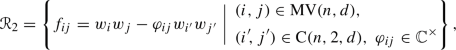  (4.2)

  where for each pair the word $w_i w_j$ occurs exactly once in , and determines uniquely a pair with , and a non-zero complex number $\varphi _{ij}$ such that , with . In particular,

  

• (3) The relations imply a set of $\left( {\begin{array}{c}N+1\\ 2\end{array}}\right)$ additional relations:

  

  (4.3)

  where for each $i < j$ the coefficient $g_{ji} = \frac{\varphi _{ji}}{\varphi _{ij}}$ is uniquely determined by the matrix ${\textbf {q}}$. We set $\varphi _{ij} = 1$ whenever $(i,j) \in {\text {C}}(n,2,d)$.

• (4) Conversely, the relations imply the relations . Moreover, is also a complete set of independent relations for the d-Veronese algebra .

Proof

(1) Suppose that $0\leqslant i<j\leqslant N$. Then $w_j > w_i$, and it is not difficult to see that $M(j) > m(i)$, so $w_jw_i$ is not in normal form. By Remark 3.5, its normal form has the shape where , and $\varphi _{ji} \in {\mathbb {C}}^{\times }$ is uniquely determined by the entries of ${\textbf {q}}$. By Lemma 4.4, $T_{\beta } = w_{i^{\prime }} w_{j^{\prime }}$ for a unique pair of ordered monomials of length d. We claim that .

Assume by contradiction that , where . This implies that . But this is possible if and only if for every $k\in \{2,\dots ,d\}$, that is , for some $p\in \{0,\dots ,n\}$, so $T_{\beta } =(x_p)^{2d}$. In other words $\beta = (\beta _0, \dots , \beta _n)$, where $\beta _p = 2d$ and $\beta _i =0$ for every $i \ne p$. One has , which together with $|w_i|=|w_j|= d$ imply $\alpha ^i =\alpha ^j$ and $w_i=w_j = (x_p)^d$, which is impossible, since by assumption $i<j$. Hence and . We know that the equality holds in , hence it is an equality in . This implies that the equality $(w_jw_i) = \varphi _{ji} w_{i^{\prime }} w_{j^{\prime }}$ holds in , for all $0 \leqslant i < j \leqslant N$. It follows that satisfies the relations $f_{ji}= 0$, for all , see (4.1). Moreover, the relations satisfy the properties given in part (1). It is clear that the order of is exactly $\left( {\begin{array}{c}N+1\\ 2\end{array}}\right)$.

(2) Suppose that $(i,j) \in {\text {MV}}(n,d)$. Then the following are equalities in :

and $\varphi _{ij} \in {\mathbb {C}}^{\times }$ is uniquely determined by the entries of ${\textbf {q}}$. By Lemma 4.4, $T_{\beta } = w_{i^{\prime }} w_{j^{\prime }}$ for a unique pair . We claim that . As in part (1), assuming that $w_{i^{\prime }}= w_{j^{\prime }}$ we obtain that $w_i=w_j = (x_p)^d$, but then , which contradicts our assumption $(i,j) \in {\text {MV}}(n,d)$. The equality holds in , therefore it is an equality in . We have shown that for every pair $(i,j) \in {\text {MV}}(n,d)$ there is unique pair such that and $w_jw_i= \varphi _{ii} w_{i^{\prime }} w_{j^{\prime }}$ holds in . Therefore satisfies the relations (4.2) from . It is clear that all properties listed in part (2) hold and . Note that

It follows that and therefore . Hence the set of relations is a disjoint union and

(4.4)

(3) Assume now that $0 \leqslant i < j \leqslant N$. Two cases are possible.

(a) $(i,j) \in {\text {C}}(n,2,d)$. In this case and $w_j w_i = \varphi _{ji} w_i w_j = \varphi _{ji} w_{i^{\prime }}w_{j^{\prime }}$, so $g_{ji}= \varphi _{ji}$.

(b) $(i,j) \in {\text {MV}}(n,d)$. Then the two relations

$$\begin{aligned} w_j w_i = \varphi _{ji} w_{i^{\prime }}w_{j^{\prime }}\quad \text{ and }\quad w_i w_j = \varphi _{ij} w_{i^{\prime }}w_{j^{\prime }} \end{aligned}$$

imply

and therefore . It follows that $w_jw_i = g_{ji}w_iw_j$, where the non-zero coefficient $g_{ji}= \frac{\varphi _{ji}}{\varphi _{ij}}$ is uniquely determined by ${\textbf {q}}$.

(4) This is analogous to (3).$\square$

Observe that Theorem 4.5 contains important numerical data about the d-Veronese , which will be used in the sequel, and which we summarise below.

Notation 4.6

Let be the quantum space defined via a multiplicatively anti-symmetric matrix ${\textbf {q}}$. Let $d \geqslant 2$ and $N = \left( {\begin{array}{c}n+d\\ n\end{array}}\right) -1$. We associate to the d-Veronese a list of invariants uniquely determined by ${\textbf {q}}$ and d.

Let ${\mathfrak {F}}_1= \{\varphi _{ji}\,{|}\, 0\leqslant i < j \leqslant N\}$ be the set of coefficients occurring in (see (4.1)) and let ${\mathfrak {F}}_2= \{\varphi _{ij}\,{|}\, (i,j) \in {\text {MV}}(n,d)\}$ be the set of coefficients occurring in (see (4.2)). Let ${{\textbf {g}}} = \Vert g_{ij}\Vert$ be the multiplicatively anti-symmetric matrix whose entries $g_{ij}$, $0 \leqslant i < j \leqslant N$, are the coefficients occurring in see (4.3). We collect this information about in the following data:

5 Veronese maps

Let $n, d\in {\mathbb {N}}$ and $N=\left( {\begin{array}{c}n+d\\ d\end{array}}\right) -1$. In this section, we introduce and study non-commutative analogues of the Veronese embeddings $V_{n,d}:{\mathbb {P}}^{\,n} \rightarrow {\mathbb {P}}^N$. The main result of the section is Theorem 5.2, which describes explicitly the reduced Gröbner bases for the kernel of the non-commutative Veronese map.

We keep the notation and conventions from the previous sections, so $X_n = \{x_0, \dots , x_n\}$ and is the set of ordered monomials (terms) in the alphabet $X_n$. The set of all degree d terms is enumerated according the degree-lexicographic order in $\langle X_n \rangle$:

We introduce a second set of variables $Y_N = \{y_0, \dots , y_N\}$, and given an arbitrary multiplicatively anti-symmetric matrix ${{\textbf {g}}} =\Vert g_{ij}\Vert$, we present the corresponding quantum space as , where

5.1 Definitions and first results

Lemma 5.1

Let $n, d\in {\mathbb {N}}$ and let $N=\left( {\begin{array}{c}n+d\\ d\end{array}}\right) -1$. Let and $\;Y_N$ be as above. For every multiplicatively anti-symmetric matrix ${\textbf {q}}$, there exists a unique multiplicatively anti-symmetric matrix ${{\textbf {g}}} =\Vert g_{ij}\Vert$ such that the assignment

$$\begin{aligned} y_0 \mapsto w_0, \;\; y_1 \mapsto w_1, \;\; \dots , \;\; y_N \mapsto w_N \end{aligned}$$

extends to an algebra homomorphism

The entries of ${{\textbf {g}}}$ are given explicitly in terms of the data of the d-Veronese , see 4.6. The image of the map $v_{n,d}$ is the d-Veronese subalgebra .

We call $v_{n,d}$ the (n, d)-Veronese map.

Proof

Suppose ${\textbf {q}}$ is an multiplicatively anti-symmetric matrix, and let be the corresponding quantum space. Assume that there exists an multiplicatively anti-symmetric matrix ${{\textbf {g}}}$ such that the map $v_{n,d}$ is a homomorphism of ${\mathbb {C}}$-algebras. Then

$$\begin{aligned} w_jw_i=v_{n,d}(y_jy_i)= v_{n,d}(g_{ji} y_iy_j)=g_{ji}w_iw_j, \end{aligned}$$

for every $0 \leqslant i \leqslant j \leqslant N$. By Theorem 4.5,

$$\begin{aligned} w_j w_i = \varphi _{ji} T_{\beta }\quad \text{ and }\quad w_i w_j = \varphi _{ij} T_{\beta }, \end{aligned}$$

for every $0 \leqslant i<j \leqslant N$, where is the unique ordered monomial of multi-degree . In the particular cases when $(i,j) \in {\text {C}}(n,2,d)$, one has $w_i w_j = T_{\beta }$, so $\varphi _{ij}= 1$. The nonzero coefficients $\varphi _{ji}$ and $\varphi _{ij}$ are uniquely determined by the matrix ${\textbf {q}}$, see 4.6. It follows that the equalities

$$\begin{aligned} \varphi _{ji} T_{\beta }= w_jw_i =g_{ji}w_iw_j = g_{ji}\varphi _{ij} T_{\beta } \end{aligned}$$

hold in , so $(g_{ji}\varphi _{ij} -\varphi _{ji}) T_{\beta } = 0$. But $T_{\beta }$ is in the ${\mathbb {C}}$-basis of , and therefore

$$\begin{aligned} g_{ji} = \frac{\varphi _{ji}}{\varphi _{ij}}\in {\mathbb {C}}^{\times }, \end{aligned}$$

(5.1)

for all $0 \leqslant i \leqslant j \leqslant N$, which agrees with 4.6. This determines a unique multiplicatively anti-symmetric matrix ${{\textbf {g}}}$ with the required properties, and therefore the quantum space is also uniquely determined. The image of $v_{n,d}$ is the subalgebra of generated by the ordered monomials , which by Theorem 4.5 is exactly the d-Veronese .

Conversely, if ${{\textbf {g}}} =\Vert g_{ij}\Vert$ is an matrix whose entries satisfy (5.1) then ${{\textbf {g}}}$ is a multiplicatively anti-symmetric matrix which determines a quantum space and the Veronese map , $y_i \mapsto w_i, 0\leqslant i \leqslant N$, is well-defined.$\square$

We fix an multiplicatively anti-symmetric matrix ${\textbf {q}}$ defining the quantum space . Let be the quantum space defined via the matrix ${{\textbf {g}}}$ from Lemma 5.1. To simplify notation, as in the previous subsection, we shall write . We know that there is a standard finite presentation , where

(5.2)

is the reduced Gröbner basis of the ideal , where $\rho$ is the canonical projection

We can lift the Veronese map to a uniquely determined homomorphism extending the assignment

$$\begin{aligned} y_0 \mapsto w_0,\; y_1 \mapsto w_1,\; \dots ,\; y_N \mapsto w_N. \end{aligned}$$

It is clear that the map V is surjective, since the restriction is bijective, and the set of ordered monomials generates .

Let . We want to find the reduced Gröbner basis of the ideal K with respect to the degree-lexicographic order $\prec$ on $\langle Y_N \rangle$, where $y_0 \prec \cdots \prec y_N$.

Heuristically, we use the explicit information on the d-Veronese subalgebra given in terms of generators and relations in Theorem 4.5, (4.1), and (4.2). In each of these relations we replace $w_i$ with $y_i$, $0\leqslant i \leqslant N$, preserving the remaining data (the coefficients and the sets of indices), and obtain a polynomial in ${\mathbb {C}}\langle Y_N \rangle$. This yields two disjoint sets of linearly independent quadratic binomials $\Re _1$ and $\Re _2$ in ${\mathbb {C}}\langle Y_N \rangle$:

• The set $\Re _1$, corresponding to the set defined in (4.1), consists of $\left( {\begin{array}{c}N+1\\ 2\end{array}}\right)$ quadratic relations:

  

  (5.3)

• The set $\Re _2$, corresponding to the set defined in (4.2), has exactly $\left( {\begin{array}{c}N+2\\ 2\end{array}}\right) - \left( {\begin{array}{c}n+2d\\ n\end{array}}\right)$ relations:

  

  (5.4)

There is one more set which is contained in K: the set of defining relations for . Note that corresponds exactly to from (4.3). We set $\Re = \Re _1\cup \Re _2$ and . It is not difficult to see that there are equalities of ideals in ${\mathbb {C}}\langle Y_N \rangle$:

and that the set of relations $\Re$ and $\Re ^{\prime }$ are equivalent.

It is clear that the set $\Re = \Re _1\cup \Re _2$ of quadratic polynomials in ${\mathbb {C}}\langle Y_N \rangle$ and the set of relations of the d-Veronese subalgebra from Theorem 4.5 have the same cardinality. In fact

(5.5)

as computed in (4.4). We shall prove that the set $\Re = \Re _1\cup \Re _2$ is the reduced Gröbner basis of K, while $\Re ^{\prime }$ is a minimal Gröbner basis of K.

Theorem 5.2

With notation as above, let be the algebra homomorphism extending the assignment

$$\begin{aligned} y_0 \mapsto w_0,\; y_1 \mapsto w_1, \; \dots , \; y_N \mapsto w_N, \end{aligned}$$

let K be the kernel of V. Let $\Re = \Re _1 \cup \Re _2$ be the set of quadratic polynomials given in (5.3) and (5.4), and let , where is given in (5.2). Then

• (1) $\Re$ is the reduced Gröbner basis of the ideal K.

• (2) $\Re ^{\prime }$ is a minimal Gröbner basis of the ideal K.

Proof

We start with a general observation. The quantum space is a quadratic algebra, therefore its d-Veronese is also quadratic, see Remark 4.2. Hence K is generated by quadratic polynomials and it is graded by length.

Remark 5.3

It is clear that the sets of leading monomials and the sets of normal monomials satisfy the following equalities in $\langle Y_N \rangle$:

Therefore $\Re ^{\prime }$ is a minimal Gröbner basis of the ideal K if and only if $\Re$ is a reduced Gröbner basis of K.

By Theorem 4.5, the quadratic polynomials $F_{ji}(Y_n)$ in (5.3) and $F_{ij}(Y_n)$ in (5.4) satisfy

$$\begin{aligned} V(F_{ji}(y_0, \dotsc , y_N)) = f_{ji}(w_0, \dotsc , w_N) = 0,\quad \text{ for } \text{ every }\;\; 0 \leqslant i < j \leqslant N, \end{aligned}$$

and

$$\begin{aligned} V(F_{ij}(y_0, \dotsc , y_N)) = f_{ij}(w_0, \dotsc , w_N) = 0,\quad \text{ for } \text{ every }\;\;(i,j) \in {\text {MV}}(n,d). \end{aligned}$$

Thus $\Re \subset K$ and, in a similar way, . We shall show that $\Re$ is a reduced Gröbner basis of K.

As usual, $N(K) \subset {\mathbb {C}}\langle Y_N \rangle$ denotes the set of normal monomials modulo K, and $N(\Re ) \subset {\mathbb {C}}\langle Y_N \rangle$ denotes the set of normal words modulo $\Re$. In general,

$$\begin{aligned} N(K) \subseteq N(\Re ), \end{aligned}$$

and by Corollary 2.6 equality holds if and only if $\Re$ is a Gröbner basis of K. Recall from Sect. 2.3 that there are isomorphisms of vector spaces

The ideal K is graded by length, i.e. $K = \bigoplus _{j \geqslant 0} K_j$, with $K_0 = K_1 = 0$.

For $j\geqslant 0$, let $N(K)_j$ be the set of normal words of length j, with the convention that $N(K)_0 = \{1\}$, $N(K)_1 = Y_N$. As vector spaces,

In particular, , so

We know that

where $Y_N^2$ is the set of all words of length two in $\langle Y_N \rangle$. This, together with (5.5), implies

$$\begin{aligned} \dim K_2 =(N+1)^2 -\left( {\begin{array}{c}n +2d\\ n\end{array}}\right) = |\Re |. \end{aligned}$$

Clearly, the set $\Re$ consists of linearly independent polynomials, therefore $\dim K_2 = \dim {\mathbb {C}}\Re = |\Re |$. It follows that ${\mathbb {C}}\Re = K_2,$ and since K is generated by quadratic polynomials, one has $K = (\Re )$.

We shall use the following remark.

Remark 5.4

The following are equivalent:

• (1) $y_iy_jy_k \in N(\Re )_3$;

• (2) $y_iy_j \in N(\Re )_2$ and $y_jy_k \in N(\Re )_2$;

• (3) $(i,j,k) \in {\text {C}}(n,3, d)$.

Moreover, there are equalities

$$\begin{aligned} |N(\Re )_3|= |{\text {C}}(n,3, d)| = \left( {\begin{array}{c}n+3d\\ n\end{array}}\right) . \end{aligned}$$

(5.6)

We know that , so which together with (5.6) imply

It follows from Lemma 2.7 that the set $\Re$ is a Gröbner basis of the ideal K. The set of leading monomials is an antichain of monomials, hence $\Re$ is a minimal Gröbner basis. For $j > i$, every $F_{ji} \in \Re$ defined in (5.3) is in normal form modulo . Similarly, for $(i,j) \in {\text {MV}}(n,d)$, every $F_{ij} \in \Re$ defined in (5.4) is in normal form modulo . We have proven that $\Re$ is a reduced Gröbner basis of the ideal K.

It follows from Remark 5.3 that $\Re ^{\prime }$ is a minimal Gröbner basis of K.$\square$

5.2 The Veronese map $v_{n,d}$ and the reduced Gröbner basis of its kernel

Theorem 5.5

Let $n, d\in {\mathbb {N}}$ and $N=\left( {\begin{array}{c}n+d\\ d\end{array}}\right) -1$. Let be a quantum space defined by an deformation matrix ${\textbf {q}}$ and let be the quantum space whose multiplicatively anti-symmetric matrix ${{\textbf {g}}}$ is determined by Lemma 5.1. Let

be the Veronese map extending the assignment

$$\begin{aligned} y_0 \mapsto w_0, \; y_1 \mapsto w_1, \; \dotsc ,\; y_N \mapsto w_N. \end{aligned}$$

• (1) The image of $v_{n,d}$ is the d-Veronese subalgebra of .

• (2) The kernel of the Veronese map has a reduced Gröbner basis consisting of exactly $\left( {\begin{array}{c}N+2\\ 2\end{array}}\right) - \left( {\begin{array}{c}n+2d\\ n\end{array}}\right)$ binomials:

  

  (5.7)

  where , $y_iy_j \succ y_{i^{\prime }}y_{j^{\prime }}$, and $\varphi _{ij} \in {\mathbb {C}}^{\times }$ are invariants of given in Notation 4.6.

Proof

Part (1) follows from Lemma 5.1. For part (2), we first prove that the set generates ${\mathfrak {K}}$. The proof is similar to the argument describing the kernel $K = \ker V$ in Theorem 5.2.

Note that . Indeed, by direct computation, one shows that the set of relations of the d-Veronese given in (4.2), so . Moreover, it follows from (5.7) that for each pair $(i,j) \in {\text {MV}}(n,d)$ the set contains exactly one element, namely $y_i y_j - \varphi _{ij} y_{i^{\prime }}y_{j^{\prime }}$, where . Here we consider the normal form , see Theorem 4.5 (2). Hence

where the last equality follows from Lemma 4.4. By Convention 3.9, we identify . Our goal is to show that the two set of normal words $N({\mathfrak {K}})$ and coincide, where

as in Definition 3.11. There are obvious isomorphisms of vector spaces

For simplicity of notation, we set and consider the canonical grading of B induced by the grading of . Then

so there are equalities

(5.8)

for every $m\geqslant 2$. In particular, for $m =2$ one has and

which implies

It is clear that the set is linearly independent, so it is a basis of the graded component ${\mathfrak {K}}_2$, and $\mathfrak {K}_2 = {\mathbb {C}}{\mathscr {R}}_{\textbf {q}} ^{{\text {v}}}$. But the ideal ${\mathfrak {K}}$ is generated by homogeneous polynomials of degree 2, therefore

(5.9)

so generates the kernel ${\mathfrak {K}}$.

We are now ready to prove that is a Gröbner basis of ${\mathfrak {K}}$. We shall provide two proofs. $\square$

First proof

Here we use an analogue of Remark 5.4 in the settings of a quantum space.

Remark 5.6

The following are equivalent:

• (1) ;

• (2) 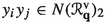and ;

• (3) $(i,j,k) \in {\text {C}}(n,3, d)$.

Moreover there are equalities

(5.10)

By (5.8), , which together with (5.10) implies

Now Lemma 3.14 implies that is a Gröbner basis of the ideal . It is clear that is the reduced Gröbner basis of ${\mathfrak {K}}$.$\square$

Second proof

We shall use Theorem 5.2 and ideas from [37]. By (5.9), we know that the set generates ${\mathfrak {K}}$. Consider now the ideal in ${\mathbb {C}}\langle Y_N \rangle$. It is easy to see that

where $K= \ker V$ is the kernel of the epimorphism from Theorem 5.2. Indeed, the polynomials in and , considered as elements of the free associative algebra ${\mathbb {C}}\langle Y_N \rangle$, satisfy

where $\Re _1^{\prime }$ and $\Re _2$ are the relations given in Theorem  5.2, see (4.3) and (5.4). Hence by the same theorem, the set is a minimal Gröbner basis of the ideal K. Theorem 5.2 also implies that the disjoint union of quadratic relations $\Re = \Re _1 \cup \Re _2$ is the reduced Gröbner basis of K in ${\mathbb {C}}\langle Y_N \rangle$. It follows from [37, Proposition 9.3 (3)] that the intersection

is the reduced Gröbner basis of the ideal . Moreover, we have . Then the obvious equalities

imply that is the reduced Gröbner basis of ${\mathfrak {K}}$. $\square$

We remark that [37, Proposition 9.3 (4)] implies that the set is the reduced Gröbner basis of the ideal K. This fact agrees with Part (3) of our Theorem 5.2, proven independently.

Corollary 5.7

The set of leading monomials for the Gröbner basis does not depend on the deformation matrix ${\textbf {q}}$ and equals

6 Segre products and Segre maps

In this section we introduce and investigate non-commutative analogues of the Segre embedding The main result of the section is Theorem 6.10, which describes explicitly the reduced Gröbner basis for the kernel of the non-commutative Segre map. We first recall the notion of Segre product of graded algebras, following [38, Sect. 3.2].

Definition 6.1

Let

$$\begin{aligned} R=\bigoplus _{k\in {\mathbb {N}}_0}R_k\quad \text{ and }\quad S=\bigoplus _{k\in {\mathbb {N}}_0}S_k \end{aligned}$$

be graded algebras. The Segre product of R and S is the graded algebra

Clearly, the Segre product is a subalgebra of the tensor product algebra . Note that the embedding is not a graded algebra morphism, as it doubles grading. The Hilbert function of satisfies

Given $n, m \in {\mathbb {N}}$, let

Let ${\textbf {q}}$ and ${\textbf {q}} ^{\prime }$ be two multiplicatively anti-symmetric matrices of sizes and , respectively, and let and be the corresponding quantum spaces. We shall construct a quantum space defined via $N+1$ (double indexed) generators

$$\begin{aligned} Z_{nm}= \bigl \{z_{i\alpha }\mid i\in \{0,\dots ,n\},\, \alpha \in \{0,\dots ,m\}\bigr \} \end{aligned}$$

and an multiplicatively anti-symmetric matrix ${{\textbf {g}}}$ uniquely determined by ${\textbf {q}}$ and ${\textbf {q}} ^{\prime }$.

Convention 6.2

We order the set $Z_{nm}$ using the lexicographic ordering on the pairs of indices $(i, \alpha )$, $0 \leqslant i \leqslant n$, $0 \leqslant \alpha \leqslant m$, that is, $z_{i\alpha } \prec z_{j\beta }$ if and only if either (a) $i < j$, or (b) $i = j,$ and $\alpha < \beta$. Thus

$$\begin{aligned} Z_{nm} = \{z_{00} \prec z_{01} \prec \cdots \prec z_{0m} \prec z_{10}\prec \cdots \prec z_{nm-1 } \prec z_{nm} \}. \end{aligned}$$

(6.1)

When no confusion arises, we write Z for $Z_{nm}$. As usual, we consider the free associative algebra ${\mathbb {C}}\langle Z \rangle$ and fix the degree-lexicographic ordering $\prec$ induced by (6.1) on the free monoid $\langle Z \rangle$.

In this section, we shall work simultaneously with three disjoint sets of variables, $X= X_n$, $Y =Y_m$, and $Z = Z_{nm}$. We shall use notation , and for the corresponding sets of ordered terms in variables X, respectively Y, respectively Z. In particular, the set of ordered monomials in Z with respect to the ordering (6.1) is

As in Convention 3.9, we identify with and with .

Remark 6.3

Consider the free associative algebra ${\mathbb {C}}\langle X;Y \rangle = {\mathbb {C}}\langle x_0, \dotsc , x_n, y_0, \dotsc , y_m\rangle$, generated by the disjoint union $X_n \sqcup Y_m$, and the free monoid $\langle X;Y \rangle = \langle x_0, \dotsc , x_n, y_0,\dotsc , y_m\rangle$ with the canonical degree-lexicographic ordering $\prec$ extending $x_0\prec x_1 \prec \cdots \prec x_n\prec y_0 \prec y_1 \prec \cdots \prec y_m$. Let

Then is the reduced Gröbner basis of the two-sided ideal of ${\mathbb {C}}\langle X;Y \rangle$ and there is an isomorphism of algebras

Proposition 6.4

In notation as above, let and be quantum spaces and let . Then there exists a unique multiplicatively anti-symmetric matrix ${{\textbf {g}}} =\Vert g_{i\alpha , j\beta }\Vert$ such that the assignment

extends to a well-defined ${\mathbb {C}}$-algebra homomorphism

(6.2)

Moreover, the following conditions hold:

• (1) The quantum space is presented as

  

  where

  

  is a reduced Gröbner basis for the two-sided ideal in ${\mathbb {C}}\langle Z \rangle$.

• (2) There is an isomorphism of algebras , where the multiplication $\bullet$ is defined as .

• (3) The image is the Segre subalgebra of .

We call the homomorphism $s_{n,m}$ the (n, m)-Segre map.

Proof

Assume that there exists an multiplicatively anti-symmetric matrix ${{\textbf {g}}}$ such that $s_{n,m}$ is a homomorphism of ${\mathbb {C}}$-algebras. Let $Z=Z_{nm}$ as above be the set of generators of . We compute $s_{n,m}(z_{i\alpha } z_{j\beta })$ in two different ways:

Therefore,

for every $i,j\in \{0,\dots ,n\}$ and every $\alpha ,\beta \in \{0,\dots ,m\}$. It follows that ${{\textbf {g}}} = \Vert g_{i\alpha , j \beta }\Vert$ is a multiplicatively anti-symmetric matrix uniquely determined by the equalities

$$\begin{aligned} g_{i\alpha , j \beta } = (q_{ji} q^{\prime }_{\beta \alpha })^{-1} = q_{ij} q^{\prime }_{\alpha \beta }. \end{aligned}$$

(6.3)

We remark that the matrix ${{\textbf {g}}}$ is equal to the the Kronecker product of the matrices ${\textbf {q}}$ and ${\textbf {q}} ^{\prime }$.

Conversely, if ${{\textbf {g}}}$ is the multiplicatively anti-symmetric matrix defined via (6.3), then the Segre map (6.2) is a well-defined algebra homomorphism. Conditions (1) and (2) follow straightforwardly from the discussion in Sect. 3, see Remarks 3.4 and Convention 3.9. The Segre subalgebra is generated by the elements for $i\in \{0,\dots ,n\}$ and $\alpha \in \{0,\dots ,m\}$. By construction , hence the image is the Segre subalgebra , which proves (3).$\square$

As usual, we identify the quantum space with , see Convention 3.9.

Remark 6.5

Being a Segre product, the algebra inherits various properties from the two algebras and . In particular, since the latter are one-generated, quadratic, and Koszul, it follows from [38, Proposition 3.2.1] that the algebra is also one-generated, quadratic, and Koszul. Clearly, the set of cardinality $N+1 = (n+1)(m+1)$ is a generating set of .

Lemma 6.6

The following equalities hold in the Segre product , for all i, j, $\alpha ,\beta$, such that $0 \leqslant i <j \leqslant n$ and $0 \leqslant \alpha < \beta \leqslant m$:

(6.4)

(6.5)

(6.6)

Remark 6.7

(1) The equalities given in Lemma 6.6 imply the following explicit list of defining relations for the quantum space :

for every $0 \leqslant i <j \leqslant n$ and every $0 \leqslant \alpha <\beta \leqslant m$.

(2) Equalities (6.5) imply that the following quadratic binomials in are in the kernel of the Segre map:

$$\begin{aligned} z_{i\beta }z_{j\alpha } - q^{\prime }_{\beta \alpha } z_{i\alpha }z_{j\beta } \in \ker s(n,m), \end{aligned}$$

for every $0 \leqslant i <j \leqslant n$ and every $0 \leqslant \alpha <\beta \leqslant m$.

Notation 6.8

We denote by ${\text {MS}}(n,m)$ the following collection of quadruples:

$$\begin{aligned} {\text {MS}}(n,m)= \bigl \{ (i,j,\beta , \alpha ) \mid 0 \leqslant i<j \leqslant n, 0 \leqslant \alpha < \beta \leqslant m\bigr \}. \end{aligned}$$

Lemma 6.9

The cardinality of MS(n, m) is

$$\begin{aligned} |\hbox {MS}(n,m)| = \left( {\begin{array}{c}n+1\\ 2\end{array}}\right) \left( {\begin{array}{c}m+1\\ 2\end{array}}\right) . \end{aligned}$$

Proof

Clearly, $|\{(i,j) \,{|}\, 0 \leqslant i<j \leqslant n\}| = \left( {\begin{array}{c}n+1\\ 2\end{array}}\right)$. Moreover, for each fixed pair (i, j), $0 \leqslant i<j \leqslant n$, the number of quadruples $\{(i,j,\beta , \alpha )\,{|}\, 0 \leqslant \alpha < \beta \leqslant m \}$ is exactly $\left( {\begin{array}{c}m+1\\ 2\end{array}}\right)$, which finishes the proof.$\square$

We keep the notation and conventions of this section, in particular we identify the quantum space with . Recall that if is an arbitrary set, then denotes the set of leading monomials

A monomial is normal modulo P if it does not contain as a subword any . The set of all normal mod P monomials in is denoted by $N_{\prec _0}(P)$, so

A criterion for a Gröbner basis F of an ideal ${\mathfrak {K}}=(F)$ in follows straightforwardly as an analogue of Lemma 3.13, in which we only replace $Y_N$ with the set of generators Z, and keep the remaining notation and assumptions.

Theorem 6.10

The set

consisting of $\left( {\begin{array}{c}n+1\\ 2\end{array}}\right) \left( {\begin{array}{c}m+1\\ 2\end{array}}\right)$ quadratic binomials is a reduced Gröbner basis for the kernel of the Segre map

Proof

It is clear that . We set

By Remark 6.7 (2), . We claim that generates ${\mathfrak {K}}$ as a two-sided ideal of .

The image is the Segre product , which is a quadratic algebra, see Remark 6.5. Therefore the kernel ${\mathfrak {K}}$ is generated by polynomials of degree 2. Moreover, there is an isomorphism of vector spaces

In particular,

It is clear that , hence

Now the equality , together with the obvious linear independence of the elements of , imply that is a ${\mathbb {C}}$-basis of $({\mathfrak {K}})_2$, so it spans the space $({\mathfrak {K}})_2$. But we know that the kernel ${\mathfrak {K}}$ is generated by polynomials of degree 2, hence .

Next we shall prove that is a Gröbner basis of the ideal ${\mathfrak {K}}$. Let . Then

Hence

(6.7)

We claim that . Indeed, by the identification we have

Clearly, a monomial is normal modulo if and only if each of its subwords of length 2, $z_{i\alpha }z_{j\beta }$ and $z_{j\beta }z_{k\gamma }$, is normal modulo . Moreover,

therefore

(6.8)

It follows from (6.8) that

which together with (6.7) give the desired equality . Now Lemma 3.14 implies that is a Gröbner basis of the ideal ${\mathfrak {K}}$. It is obvious that is a reduced Gröbner basis of ${\mathfrak {K}}$.$\square$

7 Examples

We present here some examples that illustrate the results of our paper.

Example 7.1

(The non-commutative twisted cubic curve) Let $n=1$ and $d=3$. Then

In this case $N=\left( {\begin{array}{c}1+3\\ 3\end{array}}\right) -1 =3$ and the corresponding quantum space is defined by the following data:

$$\begin{aligned} \begin{array}{l} Y= \{y_0, y_1, y_2, y_3\}, \quad { {{\textbf {g}}} }= \begin{pmatrix} 1 &{}\quad q^{-3} &{}\quad q^{-6}&{}\quad q^{-9} \\ q^3 &{}\quad 1 &{}\quad q^{-3}&{}\quad q^{-6} \\ q^6 &{}\quad q^3 &{}\quad 1&{}\quad q^{-3} \\ q^9 &{}\quad q^6 &{}\quad q^3&{}\quad 1 \\ \end{pmatrix}. \end{array} \end{aligned}$$

The kernel of the Veronese map has a reduced Gröbner basis G given below

$$\begin{aligned} G= \bigl \{y_1^2-q^2y_0y_2, \, y_1y_2-qy_0y_3, \, y_2^2-q^2y_1y_3\bigr \}. \end{aligned}$$

We have used the fact that in this case ${\text {MV}}(1,3)=\{(1,1),(1,2),(2,2)\}$.

Setting $q=1$ we obtain that the defining ideal for the commutative Veronese is generated by the three polynomials $\{y_1^2-y_0y_2,y_1y_2-y_0y_3, y_2^2-y_1y_3\}$. This is exactly the set of generators described and discussed in [27, pp. 23, 51].

Example 7.2

(The non-commutative rational normal curves) Generalising the previous example, we consider $n=1$ and d arbitrary. In notation as above, we write

In this case, $N= \left( {\begin{array}{c}d+1\\ d\end{array}}\right) -1=d$ and the corresponding quantum space is determined by the data

$$\begin{aligned} \begin{array}{l} Y= \{y_0, y_1, \dots , y_d\}, \quad {{{\textbf {g}}} }= \begin{pmatrix} 1 &{}\quad q^{-d} &{}\quad q^{-2d}&{}\quad \dots &{}\quad \dots &{}\quad \dots &{}\quad q^{-d^2} \\ q^{d} &{}\quad 1 &{}\quad q^{-d }&{}\quad &{}\quad &{}\quad &{}\quad q^{-d(d-1)} \\ q^{2d} &{}\quad q^{d} &{}\quad 1&{}\quad \ddots &{}\quad &{}\quad &{}\quad q^{-d(d-2)} \\ \vdots &{}\quad &{}\quad \ddots &{}\quad \ddots &{}\quad \ddots &{}\quad &{}\quad \vdots \\ \vdots &{}\quad &{}\quad &{}\quad \ddots &{}\quad \ddots &{}\quad \ddots &{}\quad \vdots &{}\quad \\ q^{d(d-1)} &{}\quad &{}\quad &{}\quad &{}\quad \ddots &{}\quad 1 &{}\quad q^{-d} \\ q^{d^2} &{}\quad q^{d(d-1)} &{}\quad q^{d(d-2)} &{}\quad \dots &{}\quad \dots &{}\quad q^d &{}\quad 1 \\ \end{pmatrix}. \end{array}\nonumber \\ \end{aligned}$$

(7.1)

Observe that whenever q is a d-th root of unity, the derived (1, d)-quantum space is a commutative algebra.

The kernel of the Veronese map has a reduced Gröbner basis G given by $\left( {\begin{array}{c}d\\ 2\end{array}}\right)$ quadratic relations:

$$\begin{aligned} G= \lbrace y_i y_j-h_{ij} \, \vert \, 1 \leqslant i \leqslant j \leqslant d-1 \rbrace , \quad h_{ij} = {\left\{ \begin{array}{ll}\, q^{i(d-j)} y_0 y_{i+1}, &{} i+j \leqslant d, \\ \,q^{i(d-j)}y_{i+j-d} y_d, &{} i+j > d. \end{array}\right. } \end{aligned}$$

Once again, for $q=1$ we obtain that a reduced Gröbner basis for the defining ideal of the commutative rational normal curve (see [27, Example 1.16]).

Example 7.3

(The non-commutative Veronese surface) Let $n=d=2$, that is,

In this case $N=5$ and the corresponding (2, 2)-quantum space is completely determined by the data

Observe that inside the matrix ${{\textbf {g}}}$ we find as submatrices three occurrences of the matrix in (7.1) for $d=2$ and q equal to one of the three commutation parameters, namely

$$\begin{aligned} \begin{pmatrix} 1 &{}\quad q_{10}^{-2} &{}\quad q_{10}^{-4} \\ q_{10}^{2} &{}\quad 1 &{}\quad q_{10}^{-2} \\ q_{10}^{4} &{}\quad q_{10}^{2} &{}\quad 1 \end{pmatrix}, \qquad \begin{pmatrix} 1 &{}\quad q_{20}^{-2} &{}\quad q_{20}^{-4} \\ q_{20}^{2} &{}\quad 1 &{}\quad q_{20}^{-2} \\ q_{20}^{4} &{}\quad q_{20}^{2} &{}\quad 1 \end{pmatrix}, \quad \text{ and } \quad \begin{pmatrix} 1 &{}\quad q_{21}^{-2} &{}\quad q_{21}^{-4} \\ q_{21}^{2} &{}\quad 1 &{}\quad q_{21}^{-2} \\ q_{21}^{4} &{}\quad q_{21}^{2} &{}\quad 1 \end{pmatrix}. \end{aligned}$$

The kernel of the Veronese map has a reduced Gröbner basis consisting of six quadratic polynomials

$$\begin{aligned} G = \bigl (&y_1^2 - q_{10} y_0y_3, \, y_1y_2-q_{10}y_0y_4, \, y_2^2 - q_{20}y_0y_5,\\&y_2y_3 - q_{21}^2 y_1y_4, \, y_2y_4 -q_{21}y_1y_5, \, y_4^2 -q_{21}y_3y_5 \bigr ) . \end{aligned}$$

Example 7.4

(The Segre quadric) Let $n=m=1$. Following the above conventions, we write

In this case, $N=3$ and the quantum space is determined by the data

$$\begin{aligned} \begin{array}{l} Z= \{z_{00}, z_{01}, z_{10}, z_{11} \}, \quad {{\textbf {g}}} = \begin{pmatrix} 1 &{}{q^\prime }{}^{-1} &{} q^{-1} &{} (q^\prime q)^{-1}\\ q^{\prime } &{} 1 &{} q^{-1} q^{\prime } &{} q^{-1} \\ q &{} q(q^\prime )^{-1} &{} 1 &{} (q^\prime )^{-1} \\ qq^{\prime } &{} q &{} q^{\prime } &{} 1 \\ \end{pmatrix}. \end{array} \end{aligned}$$

The kernel of the Segre map has a reduced Gröbner basis consisting of a single quadratic polynomial

$$\begin{aligned} G= \lbrace z_{01}z_{10} - q^\prime z_{00}z_{11} \rbrace . \end{aligned}$$

Example 7.5

(The non-commutative Segre threefold) Let $n=2$ and $m=1$. We consider

and

Then $N =5$ and the corresponding (2, 1)-derived quantum space is determined by the following data:

$$\begin{aligned} Z&= \{z_{00}, z_{01}, z_{10}, z_{11}, z_{20}, z_{21} \}, \\ {{\textbf {g}}}&= \begin{pmatrix} 1 &{}\quad (q^\prime )^{-1} &{}\quad q_{10}^{-1} &{}\quad (q_{10}q^\prime )^{-1} &{}\quad q_{20}^{-1} &{}\quad (q_{20}q^\prime )^{-1}\\ q^{\prime } &{}\quad 1 &{}\quad q_{10}^{-1} q^{\prime } &{}\quad q_{10}^{-1} &{}\quad q_{20}^{-1} q^{\prime } &{}\quad q_{20}^{-1}\\ q_{10} &{}\quad q_{10}(q^\prime )^{-1} &{}\quad 1 &{}\quad (q^\prime )^{-1} &{}\quad q_{21}^{-1} &{}\quad (q_{21}q^\prime )^{-1} \\ q_{10}q^{\prime } &{}\quad q_{10} &{}\quad q^{\prime } &{}\quad 1 &{}\quad q_{21}^{-1}q^{\prime } &{}\quad q_{21}^{-1}\\ q_{20} &{}\quad q_{20}(q^\prime )^{-1} &{}\quad q_{21} &{}\quad q_{21}(q^\prime )^{-1} &{}\quad 1 &{}\quad (q^{\prime })^{-1}\\ q_{20}q^\prime &{}\quad q_{20} &{}\quad q_{21} q^\prime &{}\quad q_{21} &{}\quad q^{\prime } &{}\quad \quad 1 \\ \end{pmatrix}. \end{aligned}$$

The kernel of the Segre map has a reduced Gröbner basis consisting of three quadratic polynomials

$$\begin{aligned} G= \bigl \lbrace z_{01}z_{10} - q^\prime z_{00}z_{11}, z_{01}z_{20} - q^\prime z_{00}z_{21}, z_{11}z_{20} - q^\prime z_{10}z_{21} \bigr \rbrace . \end{aligned}$$

References

Améndola, C., Faugère, J.-C., Sturmfels, B.: Moment varieties of Gaussian mixtures. J. Algebr. Stat. 7(1), 14–28 (2016)
Arici, F., Brain, S., Landi, G.: The Gysin sequence for quantum lens spaces. J. Noncommut. Geom. 9(4), 1077–1111 (2015)
Arici, F., Kaad, J., Landi, G.: Pimsner algebras and Gysin sequences from principal circle actions. J. Noncommut. Geom. 10(1), 29–64 (2016)
Artin, M., Schelter, W.F.: Graded algebras of global dimension \(3\). Adv. Math. 66(2), 171–216 (1987)
Auroux, D., Katzarkov, L., Orlov, D.: Mirror symmetry for weighted projective planes and their noncommutative deformations. Ann. Math. 167(3), 867–943 (2008)
Beggs, E.J., Brzeziński, T.: Line bundles and the Thom construction in noncommutative geometry. J. Noncommut. Geom. 8(1), 61–105 (2014)
Bengtsson, I., Życzkowski, K.: Geometry of Quantum States, 2nd edn. Cambridge University Press, Cambridge (2017)
Bergman, G.M.: The diamond lemma for ring theory. Adv. Math. 29(2), 178–218 (1978)
Brzeziński, T., Szymański, W.: The \(C^*\)-algebras of quantum lens and weighted projective spaces. J. Noncommut. Geom. 12(1), 195–215 (2018)
Ciccoli, N., Fioresi, R., Gavarini, F.: Quantization of projective homogeneous spaces and duality principle. J. Noncommut. Geom. 2(4), 449–496 (2008)
Cirio, L., Landi, G., Szabo, R.J.: Algebraic deformations of toric varieties II: noncommutative instantons. Adv. Theor. Math. Phys. 15(6), 1817–1907 (2011)
Cirio, L.S., Landi, G., Szabo, R.J.: Algebraic deformations of toric varieties I. General constructions. Adv. Math. 246, 33–88 (2013)
Connes, A., Landi, G.: Noncommutative manifolds, the instanton algebra and isospectral deformations. Comm. Math. Phys. 221(1), 141–159 (2001)
D’Andrea, F., Landi, G.: Bounded and unbounded Fredholm modules for quantum projective spaces. J. K-Theory 6(2), 231–240 (2010)
D’Andrea, F., Landi, G.: Quantum weighted projective and lens spaces. Comm. Math. Phys. 340(1), 325–353 (2015)
Eisenbud, D., Peeva, I., Sturmfels, B.: Non-commutative Gröbner bases for commutative algebras. Proc. Amer. Math. Soc. 126(3), 687–691 (1998)
Faddeev, L.D., Reshetikhin, N.Yu., Takhtajan, L.A.: Quantization of Lie groups and Lie algebras. In: Algebraic Analysis, vol. I, pp. 129–139. Academic Press, Boston (1988)
Garcia, L.D., Stillman, M., Sturmfels, B.: Algebraic geometry of Bayesian networks. J. Symbolic Comput. 39(3–4), 331–355 (2005)
García, F.D., Krutov, A., Buachalla, R.O., Somberg, P., Strung, K.R.: Positive line bundles over the irreducible quantum flag manifolds (2019). arXiv:abs/1912.08802
Gateva-Ivanova, T.: On the Noetherianity of some associative finitely presented algebras. J. Algebra 138(1), 13–35 (1991)
Gateva-Ivanova, T.: Noetherian properties and growth of some associative algebras. In: Mora, T., Traverso, C. (eds.) Effective Methods in Algebraic Geometry. Progress in Mathematics, vol. 94, pp. 143–158. Birkhäuser, Boston (1991)
Gateva-Ivanova, T.: Noetherian properties of skew polynomial rings with binomial relations. Trans. Amer. Math. Soc. 343(1), 203–219 (1994)
Gateva-Ivanova, T.: Skew polynomial rings with binomial relations. J. Algebra 185(3), 710–753 (1996)
Gateva-Ivanova, T.: Binomial skew-polynomial rings, Artin–Schelter regular rings, and binomial solutions of the Yang–Baxter equation. Serdica Math. J. 30(2–3), 431–470 (2004)
Gateva-Ivanova, T.: Quadratic algebras, Yang–Baxter equation, and Artin–Schelter regularity. Adv. Math. 230(4–6), 2152–2175 (2012)
Gateva-Ivanova, T., Van den Bergh, M.: Semigroups of \(I\)-type. J. Algebra 206(1), 97–112 (1998)
Harris, J.: Algebraic Geometry. Graduate Texts in Mathematics, vol. 133. Springer, New York (1992)
Hong, J.H., Szymański, W.: Quantum spheres and projective spaces as graph algebras. Comm. Math. Phys. 232(1), 157–188 (2002)
Kandri-Rody, A., Weispfenning, V.: Noncommutative Gröbner bases in algebras of solvable type. J. Symbolic Comput. 9(1), 1–26 (1990)
Kapustin, A., Kuznetsov, A., Orlov, D.: Noncommutative instantons and twistor transform. Comm. Math. Phys. 221(2), 385–432 (2001)
Landsberg, J.M.: Tensors: Geometry and Applications. Graduate Studies in Mathematics, vol. 128. American Mathematical Society, Providence (2012)
Latyshev, V.N.: Combinatorial Ring Theory. Izd. Mosk. Univ., Moscow (1988)
Manin, Yu.I.: Some remarks on Koszul algebras and quantum groups. Ann. Inst. Fourier (Grenoble) 37(4), 191–205 (1987)
Manin, Yu.I.: Quantum Groups and Noncommutative Geometry. Université de Montréal, Centre de Recherches Mathématiques, Montreal (1988)
Manin, Yu.I.: Topics in Noncommutative Geometry. M.B. Porter Lectures, Princeton University Press, Princeton (1991)
Mora, T.: Groebner bases in noncommutative algebras. In: Gianni, P. (ed.) Symbolic and Algebraic Computation. Lecture Notes in Computer Science, vol. 358, pp. 150–161. Springer, Berlin (1989)
Mora, T.: An introduction to commutative and noncommutative Gröbner bases. Theoret. Comput. Sci. 134(1), 131–173 (1994)
Polishchuk, A., Positselski, L.: Quadratic Algebras. University Lecture Series, vol. 37. American Mathematical Society, Providence (2005)
Priddy, S.B.: Koszul resolutions. Trans. Amer. Math. Soc. 152, 39–60 (1970)
Shelton, B., Tingey, C.: On Koszul algebras and a new construction of Artin–Schelter regular algebras. J. Algebra 241(2), 789–798 (2001)
Smith, S.P.: Maps between non-commutative spaces. Trans. Amer. Math. Soc. 356(7), 2927–2944 (2004)
Sottile, F., Sturmfels, B.: A sagbi basis for the quantum Grassmannian. J. Pure Appl. Algebra 158(2–3), 347–366 (2001)
Vaksman, L.L., Soibelman, Y.S.: Algebra of functions on the quantum group \({{\rm SU}}(n+1)\), and odd-dimensional quantum spheres. Leningrad Math. J. 2(5), 1023–1042 (1991)
Verëvkin, A.B.: On a noncommutative analogue of the category of coherent sheaves on a projective scheme. In: Algebra and Analysis. American Mathematical Society Translations: Series 2, vol. 151, pp. 41–53. American Mathematical Society, Providence (1992)
Acknowledgements
FA and FG would like to thank the Max Planck Institute for Mathematics in Bonn for their hospitality during a visit to TGI in May 2019. We would also like to thank Bernd Sturmfels for encouraging this line of research and Giovanni Landi for discussions on toric non-commutative manifolds. We express our gratitude to the anonymous referee for a careful and thorough reading of this paper and for their valuable suggestions and comments which helped to improve the text.
Funding
Open Access funding enabled and organized by Projekt DEAL.
Author information
Authors and Affiliations
Corresponding author
Additional information
Publisher's Note
Springer Nature remains neutral with regard to jurisdictional claims in published maps and institutional affiliations.
The authors acknowledge support by the Max Planck Institute for Mathematics in the Sciences (MPI MiS), Leipzig. FA was partially funded by the Netherlands Organisation of Scientific Research (NWO) under the VENI grant 016.192.237. TGI was partially supported by the Max Planck Institute for Mathematics, (MPIM), Bonn, and by Grant KP-06 N 32/1 of 07.12.2019 of the Bulgarian National Science Fund.
Rights and permissions
Open Access This article is licensed under a Creative Commons Attribution 4.0 International License, which permits use, sharing, adaptation, distribution and reproduction in any medium or format, as long as you give appropriate credit to the original author(s) and the source, provide a link to the Creative Commons licence, and indicate if changes were made. The images or other third party material in this article are included in the article’s Creative Commons licence, unless indicated otherwise in a credit line to the material. If material is not included in the article’s Creative Commons licence and your intended use is not permitted by statutory regulation or exceeds the permitted use, you will need to obtain permission directly from the copyright holder. To view a copy of this licence, visit http://creativecommons.org/licenses/by/4.0/.
About this article
Cite this article
Arici, F., Galuppi, F. & Gateva-Ivanova, T. Veronese and Segre morphisms between non-commutative projective spaces. European Journal of Mathematics 8 (Suppl 1), 235–273 (2022). https://doi.org/10.1007/s40879-022-00547-3
Received:
Revised:
Accepted:
Published:
Issue Date:
DOI: https://doi.org/10.1007/s40879-022-00547-3
Keywords
- Quadratic algebras
- Non-commutative projective spaces
- Veronese subalgebras