Explicit Deligne pairing

Abstract

We give an explicit formula for the Deligne pairing for proper and flat morphisms $f:X\rightarrow S$ of schemes, in terms of the determinant of cohomology. The whole construction is justified by an analogy with the intersection theory on non-singular projective algebraic varieties.

1 Introduction

The intersection pairing between two divisors on a projective non-singular surface is the unique bilinear and symmetric pairing with values in ${\mathbb {Z}}$ that satisfies some very natural properties: it counts the number of intersection points (when the divisors are normal crossing) and it is invariant if we “move” any of the two divisors in their linear class of equivalence. With the same philosophy, such a definition of intersection pairing between divisors can be extended naturally for projective non-singular varieties of any dimension: we list a number of natural properties and we find a unique multi-linear symmetric pairing satisfying them. It turns out that this unique intersection pairing on algebraic varieties can be expressed explicitly in terms of the Euler–Poincaré characteristics of (invertible sheaves associated to the) divisors. For example, for a surface over a field k we have the well-known formula

(1.1)

which is involved in the proof of the Riemann–Roch theorem for surfaces (see for example [1]).

For a relative scheme $X\rightarrow S$, if we do not appeal to any “compactification arguments” of X and S, there is in general no hope for finding a non-trivial reasonable intersection pairing for divisors which is invariant up linear equivalence. Let us see a simple example in the case of an arithmetic surface $X\rightarrow {{\,\mathrm{Spec}\,}}{\mathbb {Z}}$: consider a prime $p\in {{\,\mathrm{Spec}\,}}{\mathbb {Z}}$, then the fibre $X_{p}$ is a principal vertical divisor on X. Let D be an effective, irreducible, horizontal divisor on X, then certainly D meets $X_p$, so on one hand $D.X_p>0$ since our phantomatic intersection pairing should count the number of intersection points with multiplicity; but on the other hand we said that $X_p$ is principal, which means $D.X_p=0$.

The closest object to an intersection pairing on a relative scheme $X\rightarrow S$ of relative dimension n is the Deligne pairing. It is a map

where denotes the set of invertible sheaves, which descends to a symmetric, multi-linear map at the level of Picard groups. This pairing is of crucial importance in arithmetic geometry, since it gives “the schematic contribution” to the Arakelov intersection number.

The Deligne pairing was originally constructed by Deligne in [6] for arithmetic surfaces and then generalised to any dimension in [8, 9, 22]. Its definition was not built as the unique solution of a universal problem, it was rather constructed locally in terms of meromorphic sections of invertible sheaves. A set of axioms that uniquely identify the Deligne pairing have been found recently in the preprint [21].

For arithmetic surfaces one can show the following isomorphism of invertible sheaves which turns out to be crucial in the proof of Faltings–Riemann–Roch theorem (see for example [6, 16] for more details):

(1.2)

One can notice immediately the similarities between equations (1.1) and (1.2). The only substantial difference is that for algebraic surfaces we use the Euler–Poincaré characteristic, whereas for arithmetic surfaces we use the determinant of the cohomology. Such a distinction makes perfect sense, since the determinant of the cohomology is constructed to be the arithmetic analogue of the Euler–Poincaré characteristic.

At this point the natural question is the following one: is it possible to give an explicit definition of the Deligne pairing (in the most general case) in terms of the determinant of cohomology?¹ In this paper we give an affirmative answer. By working in complete analogy of the theory of algebraic varieties, we write down a simple explicit formula for the Deligne pairing in terms of the determinant of cohomology. Let $f:X\rightarrow S$ be a proper, flat morphism of integral Noetherian schemes, and assume that f has pure dimension n, then we put

(1.3)

where for any coherent sheaf ${\mathscr {F}}$ and any invertible sheaf ${\mathscr {L}}$ (here only the class of ${\mathscr {F}}$ in the Grothendieck group matters). Moreover $N_{X/S}$ is the norm, relative to f, of an invertible sheaf. We show that definition (1.3) satisfies the axioms of [21], and this implies that our definition is exactly the Deligne pairing.

Let us mention some other papers that previously investigated in our direction: an explicit formula for the Deligne pairing when X and S are integral schemes over ${\mathbb {C}}$ was announced in [3], although a complete proof is not given. The approach of [3] is essentially different from ours, indeed the authors work on local trivializations of invertible sheaves. A more complicated expression of the Deligne pairing in terms of symmetric difference of the functor $\det Rf_*$ is proved in [7] with heavy usage of category theory (see also [4, Appendix A]). Moreover, when ${\mathscr {L}}$ is very ample on the fibres, an explicit expression of the Deligne pairing $\langle \mathscr {L},\ldots ,{\mathscr {L}}\rangle$, is given in [18] as the leading term of the Knudsen–Mumford expansion of $\det Rf_*(\mathscr {L}^k)$.

This paper is organized in the following way: in Sect. 2 we introduce the map $c_1({\mathscr {L}}):K_0(X)\rightarrow K_0(X)$ with all its properties. Section 3 is a review of intersection theory for algebraic varieties and it gives to the reader the philosophical guidelines for the case of relative schemes. In Sect. 4 we give the axioms of the Deligne pairing and we show with all details that if such pairing exists, then it must be unique (we follow [21]). Afterwards we show that the pairing (1.3) satisfies all the axioms. Appendix A is a review of the determinant of cohomology, this part is crucial in order to understand Sect. 4. Finally, in Appendix B we review in all details the original construction of Deligne pairing of [6] (very often this construction is just sketched in the literature).

2 An endomomorphism of the group $K_0(X)$

Let us briefly recall the abstract construction of the Groethendieck group $K_0(\mathbf{C} )$. Fix an abelian category $\mathbf{C}$ and let $F(\mathbf{C} )$ be the free abelian group over the set ${{\,\mathrm{Ob}\,}}(\mathbf{C} )/{\cong }$, where $\cong$ is the isomorphism relation. If $C\in {{\,\mathrm{Ob}\,}}(\mathbf{C} )$, then (C) denotes isomorphism class in ${{\,\mathrm{Ob}\,}}(\mathbf{C} )/{\cong }$. To any short exact sequence in $\mathbf{C}$,

we associate an element . Now, $H(\mathbf{C} )$ is the subgroup of $F(\mathbf{C} )$ generated by all the elements $Q({\mathcal {S}})$ for ${\mathcal {S}}$ running over all short exact sequences. Then

and $[C]\in K_0(\mathbf{C} )$ denotes the equivalence class associated to $C\in {{\,\mathrm{Ob}\,}}(\mathbf{C} )$.

Let us fix a Noetherian scheme X, then , where $\mathbf{Coh} (X)$ is the category of coherent sheaves on X. From now on, by an abuse of notation we identify any coherent sheaf ${\mathscr {F}}$ with its class in $K_0(X)$. In this paper, with the notation $\mathbf{Coh} _{\,r}(X)$ we denote the category of coherent sheaves on X whose support has dimension at most r, and we define . Clearly when $0\leqslant i\leqslant j$, then $K_{0,i}(X)\subseteq K_{0,j}(X)$.

For any invertible sheaf ${\mathscr {L}}$ on X we define a map

Note that it is well defined because tensoring with an invertible sheaf is an exact functor, moreover it defines and endomorphism of the group $K_0(X)$. Since the notation for the function $c_1({\mathscr {L}})$ is multiplicative, the symbol denotes the composition of functions. The properties of the operator $c_1({\mathscr {L}})$ are well described in [12, Appendix B], so here we just recall them.

Proposition 2.1

The following properties hold for the operator $c_1({\mathscr {L}})$:

• (i) , where clearly the sum is taken in .

• (ii) .

• (iii) If $Z\subset X$ is a closed subscheme and ${\mathscr {L}}_{|Z}={\mathscr {O}}_Z(D)$ where D is an effective Cartier divisor on Z, then .

Proof

Both sides of the equality in (i) applied to ${\mathscr {F}}$ expand to

(2.1)

(ii) follows easily by looking at equation (2.1). For (iii) consider the short exact sequence

Proposition 2.2

([12, Lemma B4]) Let ${\mathscr {F}}\in K_{0,r}(X)$ and let $Z_1,\ldots , Z_s$ be the r-dimensional irreducible components of   whose generic points are denoted respectively by $z_i$. Let $n_i={{\,\mathrm{length}\,}}{\mathscr {F}}_{z_i}$. Then in $K_{0,r}(X)$ we have the equality

$$\begin{aligned}{\mathscr {F}}\equiv \sum ^s_{i=1} n_i{\mathscr {O}}_{Z_i}\;\,\mathrm{mod} \ K_{0,r-1}(X).\end{aligned}$$

Proposition 2.3

([12, Lemma B5]) Let ${\mathscr {L}}$ be an invertible sheaf on X, then $c_1(\mathscr {L})K_{0,r}(X)\subset K_{0,r-1}(X)$ for any $r\geqslant 0$.

Remark 2.4

The operator $c_1({\mathscr {L}})$ can be “extended” to bounded complexes of coherent sheaves on X. Let ${\mathscr {F}}^\bullet$ be a bounded complex of objects in $\mathbf{Coh} (X)$ then we can define

Such a map is clearly zero on short exact sequences.

3 Intersection theory for algebraic varieties

Definition 3.1

Let X be an n-dimensional projective, non-singular algebraic variety over a field k. An intersection pairing on X is a map

$$\begin{aligned} {{\,\mathrm{Div}\,}}(X)^n&\rightarrow {\mathbb {Z}}\\ (D_1,\ldots ,D_n)&\mapsto D_1.D_2.\,\ldots \,.D_n \end{aligned}$$

satisfying the following properties:

• (1) It is symmetric and ${\mathbb {Z}}$-multilinear.

• (2) It descends to a pairing .

• (3) Let $D_i$ be a prime divisor for any i and let $e_{i,x}\in {\mathscr {O}}_{X,x}$ be a local equation of $D_i$ at the point x. Assume that for all x in the support of all divisors $D_i$, the $e_{i,x}$’s form a regular sequence in $\mathscr {O}_{X,x}$ (i.e., the divisors are in general position), then

  

Now we show that if an intersection pairing exists, it is uniquely defined by the three axioms of Definition 3.1.

Proposition 3.2

If an intersection pairing exists, then it is unique.

Proof

Let and be two pairings satisfying axioms (1)–(3) and fix ; by (1) we can assume that all $D_i$ are prime. Thanks to Chow’s moving lemma we can find some divisors $D'_i$ such that $D\sim D_i'$ and $D'_1,\ldots ,D'_n$ are in general position. Therefore, by using (2) and (3) we get

The remaining part of this section is devoted to providing the explicit expression of the intersection pairing on X as in [19, 20] and later [5]; then we see that the axioms of Definition 3.1 are satisfied. Such an intersection pairing uses the endomorphism defined in Sect. 2 and the Euler–Poincaré characteristic for coherent sheaves.

We actually give a definition of the intersection pairing in a more general setting, in fact we will assume that X is a relative scheme over a scheme S, and we define a “partial” intersection number for a particular subclass of divisors.

From now on, in this section we assume that $X\rightarrow S$ is a flat and proper morphism of integral Noetherian schemes. Let us denote by $\mathbf{Coh} (X/S)$ the category of coherent sheaves on X whose schematic support is proper over a 0-dimensional subscheme of S. Moreover, $\mathbf{Coh} _{\,r}(X/S)$ is the subcategory of $\mathbf{Coh} (X/S)$ made of sheaves whose support has dimension at most r. The motivation behind the restriction to sheaves with this kind of support is that for any ${\mathscr {F}}\in \mathbf{Coh} (X/S)$ we have a well-defined notion of Euler–Poincaré characteristic. In fact, if T is the schematic support of ${\mathscr {F}}$ and $S_0=f(T)$, we know that $S_0$ is Noetherian of dimension 0, so $S_0={{\,\mathrm{Spec}\,}}A$ with A artinian; at this point we can put

When $S={{\,\mathrm{Spec}\,}}k$, then $\chi _S$ is the usual Euler–Poicaré characteristic (for coherent sheaves with proper support). Thanks to the “additivity” of $\chi _S$ with respect to short exact sequences, it is immediate to notice that we have a naturally induced group homomorphism $\chi _S:K_0(\mathbf{Coh} _{\,r}(X/S))\rightarrow {\mathbb {Z}}$.

Definition 3.3

Let $X\rightarrow S$ be as above and consider $\mathscr {F}\in \mathbf{Coh} _{\,r}(X/S)$. Then the intersection number of the invertible sheaves ${\mathscr {L}}_1,\ldots {\mathscr {L}}_r$ (with respect to ${\mathscr {F}}$) is defined as

When ${\mathscr {F}}={\mathscr {O}}_X$, which implies , we put for simplicity

Moreover if ${\mathscr {L}}_i={\mathscr {O}}_X(D_i)$ for a Cartier divisor $D_i$ on X, then

Example 3.4

If X is a surface over k and C, D are two divisors, then

The mere definitions tell us that we can intersect a number of divisors which is greater or equal to the dimension on X. On the other hand, the next lemma shows that intersection of a number of divisors which is strictly bigger than the dimension of X is always 0.

Lemma 3.5

If  , then $(\mathscr {L}_1.{\mathscr {L}}_2.\,\ldots \,.{\mathscr {L}}_{r+1},{\mathscr {F}})=0$.

Proof

It follows directly from Proposition 2.3. $\square$ $\square$

Proposition 3.6

The intersection number of ${\mathscr {L}}_1,\ldots ,{\mathscr {L}}_m$ with respect to ${\mathscr {F}}$ is a ${\mathbb {Z}}$-multilinear map in the ’s (the operation is the tensor product).

Proof

Follows by Proposition 2.1 (i) and Lemma 3.5. $\square$

Proposition 3.7

([12, Lemma B.15]) Let be a morphism of S-schemes and let , then

$$\begin{aligned} (g^*{\mathscr {L}}_1.g^*{\mathscr {L}}_2.\,\ldots \,. g^*{\mathscr {L}}_n, {\mathscr {F}})=({\mathscr {L}}_1.{\mathscr {L}}_2.\,\ldots \,. {\mathscr {L}}_n, g_*{\mathscr {F}}). \end{aligned}$$

We can give an explicit expression of the intersection number on varieties.

Proposition 3.8

Let X be a non-singular algebraic variety of dimension n over a field k. The pairing

$$\begin{aligned}(D_1,\ldots ,D_n)\mapsto D_1.D_2.\,\ldots \,.D_n\end{aligned}$$

defines the intersection number on X.

Proof

Axiom (1) is satisfied thanks to Proposition 3.6. Axiom (2) is obvious and axiom (3) is [14, IV, Theorem 2.8]. $\square$

Finally we state a proposition regarding the intersection along fibres.

Proposition 3.9

([14, VI, Proposition 2.10]) Let $s\in S$ be a closed point and let $X_s$ be the fibre over b. Assume that , then the map

$$\begin{aligned}s\mapsto ({\mathscr {L}}_1,\ldots ,{\mathscr {L}}_d; {\mathscr {O}}_{X_s})\end{aligned}$$

is locally constant on S.

4 The case of schemes over a general base

4.1 Multi-monoidal and symmetric functors

The Deligne pairing will be expressed as a collection of functors, so in this section we recall what the functorial equivalent of a multi-linear homomorphism of abelian groups is.

We assume that the reader is familiar with some basic notions of category theory and the concept of Picard groupoid. Roughly speaking, a Picard groupoid is a category where the morphisms are all invertible and moreover there is a “group-like” operation between the object of the category. A simple example is the Picard category $\mathbf{Pic} (X)$, made of all invertible sheaves on a scheme X, and where the morphisms are just the isomorphisms. The “operation” in $\mathbf{Pic} (X)$ is clearly the tensor product of invertible sheaves and the identity element is the structure sheaf. The morphisms we want to consider between Picard groupoids are monoidal functors, i.e., functors that preserve the monoidal structure of the categories.

For the remaining part of this subsection we fix two Picard groupoids and .

Definition 4.1

A monoidal functor $\mathbf{C} \rightarrow \mathbf{D}$ is a collection $(F,\epsilon , \mu )$ where , satisfying the following properties:

• $F:\mathbf{C} \rightarrow \mathbf{D}$ is a functor.

• is an isomorphism.

• is an isomorphism functorial in X and Y which satisfies associativity and unitality in the obvious categorical sense.

For simplicity we often omit $\epsilon$ and $\mu$ and we say that F is a monoidal functor between $\mathbf{C}$ and $\mathbf{D}$. In symbols we write $F\in L^1(\mathbf{C} ,\mathbf{D} )$.

Definition 4.2

A natural transformation between monoidal functors $(F, \epsilon ,\mu )$ and is a monoidal natural transformation $\alpha :F\rightarrow F'$ which maps $\epsilon$ to $\epsilon '$ and $\mu$ to $\mu '$.

In order to give the next definition we need to introduce some notations. An object of the category $\mathbf{C} ^n$ (i.e., an n-uple of objects of $\mathbf{C}$) is denoted by $X=(X_1,\ldots , X_n)$. Let $X, Y\in \mathbf{C} ^n$ and let $i\in \{1,\ldots ,n\}$ be such that for any $j\in \{1,\ldots ,n\}$ with $j\ne i$ we have , then we define in the following way:

Definition 4.3

A multi-monoidal²functor $\mathbf{C} ^n\rightarrow \mathbf{D}$ is the datum of

• A functor $F:\mathbf{C} ^n\rightarrow \mathbf{D}$.

• For any functor $F':\mathbf{C} \rightarrow \mathbf{D}$ obtained by fixing $n-1$ components in $\mathbf{C}$, we have a collection $\mu '$ such that is a monoidal functor $\mathbf{C}$ and $\mathbf{D}$.

• For every $i,j\in \{1,\ldots , n\}$ and $X,Y,Z,W\in \mathbf{C} ^n$ such that $X_k=Y_k=Z_k=W_k$ for all $k\ne i,j$, we have a commutative diagram

  

The notion of symmetry is what one expects.

Definition 4.4

A multi-monoidal functor $\mathbf{C} ^n\rightarrow \mathbf{D}$ is symmetric if for any $c_i\in \mathbf{C}$ and any permutation $\Sigma \in \Sigma _n$ we have $F(c_1,\ldots c_n)\cong F(c_{\Sigma (1)},\ldots c_{\Sigma (n)})$.

The set of symmetric multi-monoidal functors from $\mathbf{C} ^n$ to $\mathbf{D}$ is denoted by $L^n(\mathbf{C} ,\mathbf{D} )$.

Definition 4.5

A natural transformation between two multi-monoidal functors is a functorial isomorphism $\alpha :F\rightarrow F'$ which restricts to a natural transformation to each component in the sense of Definition 4.2.

4.2 Axiomatic Deligne pairing

The Deligne pairing was introduced in [6] as a bilinear and symmetric map , where $X\rightarrow S$ is an arithmetic surface. Such a definition requires the choice of meromorphic sections “behaving well" on an open set, and then clearly one has to show the independence with respect to this choice. The Deligne pairing satisfies some compatibility conditions with respect to the base change, the pullback functor and the norm functor. In [8], Deligne’s construction was extended straight away for proper flat morphisms of integral schemes of any dimension.

Let $f:X\rightarrow S$ be a proper flat morphism between Noetherian integral schemes, the guiding idea of this paper is that the Deligne pairing relative to f should be a generalisation of the intersection pairing described in Sect. 3. We want to work in complete analogy with the case of algebraic varieties, so in this section we give a set of “natural axioms” that uniquely define the Deligne pairing.³ The explicit construction of the Deligne pairing will be carried out in Sect. 4.3.

Let X and S be two Noetherian integral schemes, by the symbol ${\mathcal {F}}^n(X,S)$ we denote the set of all proper flat morphisms $X\rightarrow S$ of pure dimension n.

Definition 4.6

A Deligne pairing consists of the following data for any $f\in {\mathcal {F}}^n(X,S)$ where X and S are two Noetherian integral schemes: a functor

and a collection of natural transformations $\alpha ,\beta ,\gamma ,\delta$ described below:

• (1) For any commutative square given by a base change which is proper, flat and with connected fibres

  

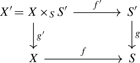
  a natural transformation $\alpha _{f,g}$ between multi-monoidal functors $\mathbf{Pic} (X)^{n+1}\rightarrow \mathbf{Pic} (S')$ such that

  

• (2) When $n>0$ and $D\in {{\,\mathrm{Div}\,}}(X)$ is an effective relative Cartier divisor, a natural transformation $\beta _{f,D}$ between multi-monoidal functors $\mathbf{Pic} (X)^{n}\rightarrow \mathbf{Pic} (S)$ such that

  $$\begin{aligned}\beta _{f,D}:\langle {\mathscr {L}}_1,\ldots ,{\mathscr {L}}_n, {\mathscr {O}}_X(D)\rangle _{X/S}\xrightarrow { \ \cong \ }\langle {\mathscr {L}}_1|_D,\ldots ,{\mathscr {L}}_n|_D\rangle _{D/S}.\end{aligned}$$

  Moreover $\beta _{f,D}$ is natural with respect to base change in the following sense: for a base change diagram as in axiom (1) we have a commutative diagram

  

  where the vertical isomorphisms are given by $\alpha _{f,g}$ (remember that $g'^*{\mathscr {O}}_X(D)={\mathscr {O}}_{X'}(g'^*D)$).

• (3) When $n>0$, a natural transformation $\gamma _{f}$ between multi-monoidal functors such that

  $$\begin{aligned}\gamma _{f}:\langle f^*{\mathscr {L}},{\mathscr {L}}_1\ldots ,{\mathscr {L}}_n\rangle _{X/S}\xrightarrow { \ \cong \ }{\mathscr {L}}^{({\mathscr {L}}_1|_{X_s}.{\mathscr {L}}_2|_{X_s}.\,\ldots \,.{\mathscr {L}}_n|_{X_s};{\mathscr {O}}_{X_s})}\end{aligned}$$

  where $X_s$ is a generic fibre of f (see Proposition 3.9). Moreover $\gamma _{f}$ is natural with respect to base change in the following sense: for a base change diagram as in axiom (1) we have a commutative diagram

  

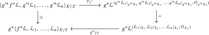
  where the vertical isomorphism is given by $\alpha _{f,g}$ and the equality follows from Proposition 3.7 and the properties of g.

• (4) When $n=0$, a natural transformation $\delta _{f}$ between monoidal functors $\mathbf{Pic} (X)\rightarrow \mathbf{Pic} (S)$ such that

  $$\begin{aligned}\delta _{f}:\langle {\mathscr {L}}\rangle _{X/S}\xrightarrow { \ \cong \ } N_{X/S}({\mathscr {L}})\end{aligned}$$

  where $N_{X/S}$ is the norm of f (see Definition A.7). Moreover, $\delta _f$ is natural with respect to base change in the following sense: for a base change diagram as in axiom (1) we have a commutative diagram

  

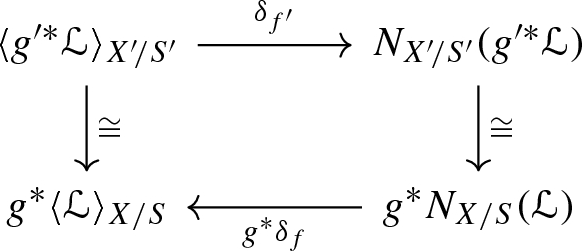
  where the vertical isomorphisms are given respectively by $\alpha _{f,g}$ and thanks to the properties of the norm.

We have to show that if a Deligne pairing exists, then it is unique. Roughly speaking, we will show that any two pairings , with $i=1,2$, satisfying the axioms of Definition 4.6 are related by natural transformation of functors that respects all the data. We will work by induction on the relative dimension of the morphism f. Note that we cannot use straight away property (2) to pass from relative dimension n to $n-1$, since the whole construction would depend on the choice of a relative divisor D, whereas we want our constructions to be natural in a functorial way. So, let us describe a general well-known procedure to reduce the relative dimension of f by using a canonical choice of a relative Cartier divisor. It is called universal extension.

Let $f\in {\mathcal {F}}^n(X,S)$ and let ${\mathscr {L}}$ be an invertible sheaf on X. We assume that ${\mathscr {L}}$ is sufficiently ample with respect to f, i.e., that the following properties are satisfied: ${\mathscr {L}}$ is very ample with respect to f and $R^i f_*{\mathscr {L}}=0$ for $i>0$.

Remark 4.7

The following properties hold for sufficient ampleness:

• It is preserved after base change.

• If $f\in {\mathcal {F}}^n(X,S)$ and ${\mathscr {L}}$ is sufficiently ample on X, then $f_*{\mathscr {L}}$ is a locally free sheaf on S.

• If ${\mathscr {L}}_0$ is an invertible sheaf on X, then there exists a sufficiently ample ${\mathscr {L}}$ such that is sufficiently ample. In particular we can always find on X a sufficiently ample invertible sheaf.

Put ${\mathscr {M}}=(f_*{\mathscr {L}})^{\vee }$ and let be the projective vector bundle associated to ${\mathscr {M}}$, over S. Then we obtain the following base change diagram:

Consider now the invertible sheaf on ${\mathbb {X}}$. We want to construct a canonical global section $\Sigma$ of ${\mathscr {L}}_f$. It is enough to find a canonical non-zero element in ${\mathscr {L}}^{-1}_f$, because if $\phi \in {{\,\mathrm{Hom}\,}}({\mathscr {O}}_X,{\mathscr {L}}_f)=\mathscr {L}^{-1}_f$ then we put . First of all we construct a surjective canonical morphism

$$\begin{aligned} \Psi :f^*{\mathscr {M}}\rightarrow {\mathscr {L}} . \end{aligned}$$

Thanks to the properties of the pullback we have a canonical isomorphism . Since ${\mathscr {L}}$ is sufficiently ample, we have a canonical isomorphism . Moreover there is a surjective canonical map given in the following way:

By taking all compositions, we finally get our surjective $\Psi$. We have to prove that $\Psi$ induces a canonical element in $\mathscr {L}^{-1}_f$ (in order to get $\Sigma$). Note that ${\mathscr {L}}^{-1}_f$ is canonically isomorphic to , but

We conclude that the dual map of $\Psi$ induces the non-zero element of ${\mathscr {L}}^{-1}_f$ that we were searching for.

From now on we will say that the section $\Sigma$ constructed above is the universal section relative to ${\mathscr {L}}$. The following remark explains why we can use the universal section for our inductive step in the proof of uniqueness.

Remark 4.8

In [9, 2.2] it is shown that $\Sigma$ is a regular section, which is equivalent to say that the zero locus of $\Sigma$ (considered with its reduced scheme structure)

is a relative Cartier divisor on ${\mathbb {X}}$. In this case we also have that ${\mathscr {L}}_f$ is canonically isomorphic to $\mathscr {O}_{{\mathbb {X}}}(Z(\Sigma ))$. Now consider the restriction

Let U be the flat locus of p and put . Then V is open in ${\mathbb {P}}$, and we denote its closed complement by W, then we conclude that

$$\begin{aligned} p:Z(\Sigma )-p^{-1}(W)\rightarrow V \end{aligned}$$

(4.2)

is flat of relative dimension $n-1$.

The following theorem ensures the unicity of the Deligne pairing.

Theorem 4.9

The Deligne pairing is unique: given two sets of data , with $i=1,2$, satisfying the conditions of Definition 4.6, there is a unique multi-monoidal morphism that transforms accordingly.

Proof

We proceed by induction on n. When $n=0$, the claim follows directly from axiom (4). Let us work now with $n>0$; first of all we want a functorial isomorphism

$$\begin{aligned} \Psi ({\mathscr {L}}_0,\ldots , {\mathscr {L}}_n):\langle \mathscr {L}_0,\ldots ,{\mathscr {L}}_n\rangle ^1_{X/S}\xrightarrow { \ \cong \ }\langle {\mathscr {L}}_0,\ldots ,{\mathscr {L}}_n\rangle ^2_{X/S}. \end{aligned}$$

(4.3)

Let us first construct it by assuming that one invertible sheaf ${\mathscr {L}}={\mathscr {L}}_0$ is chosen sufficiently ample; we will denote it by $\Psi '({\mathscr {L}}_0,\ldots , {\mathscr {L}}_n)$. Let us construct for ${\mathscr {L}}$ the base change diagram (4.1), with the same notations. Then $\Sigma$ is the universal section of ${\mathscr {L}}_f$ and we also have the map p described in equation (4.2). Thanks to [10, Lemme 21.13.2], in order to give isomorphism (4.3), it is enough to give a functorial isomorphism

$$\begin{aligned} (\pi |_{V})^*\langle {\mathscr {L}}, {\mathscr {L}}_1,,\ldots ,\mathscr {L}_n\rangle ^1_{({\mathbb {X}}-p_1^{-1}(W))/V}\xrightarrow {\ \cong \ }(\pi |_{V})^*\langle {\mathscr {L}},{\mathscr {L}}_1,\ldots ,\mathscr {L}_n\rangle ^2_{({\mathbb {X}}-p_1^{-1}(W))/V}, \end{aligned}$$

where $V\subset {\mathbb {P}}$ is the image of the flat locus of p (remember that V is open) and $W={\mathbb {P}}-V$. Let us now put . By applying axiom (1), it is enough to get a functorial isomorphism

Now remember that by definition of ${\mathscr {L}}_f$ we have

Let us put for simplicity of notations ; by multi-additivity and axiom (3) we only need to find a functorial isomorphism

At this point put ; thanks to axiom (2), it is enough to find a functorial isomorphism

$$\begin{aligned} \begin{aligned} \langle (q^*{\mathscr {L}}_1)|_{Z'(\Sigma )},&\ldots ,(q^*\mathscr {L}_n)|_{Z'(\Sigma )}\rangle ^1_{Z'(\Sigma )/V}\\&\xrightarrow { \ \cong \ }\langle (q^*\mathscr {L}_1)|_{Z'(\Sigma )},\ldots ,(q^*{\mathscr {L}}_n)|_{Z'(\Sigma )}\rangle ^2_{Z'(\Sigma )/V}. \end{aligned} \end{aligned}$$

The relative dimension of the map $p:Z'(\Sigma )\rightarrow V$ is now $n-1$ and we can apply the inductive hypothesis.

We still have to prove the existence of $\Psi ({\mathscr {L}}_0,\ldots , {\mathscr {L}}_n)$ for a general ${\mathscr {L}}_0$. For any invertible sheaf ${\mathscr {L}}_0$ there exists a sufficiently ample one $\mathscr {M}$ such that is again sufficiently ample. So we can put

provided that the construction does not depend on the choice of ${\mathscr {M}}$. Such a claim is equivalent to showing that is additive with respect to sufficiently ample invertible sheaves.

Now we consider two sufficiently ample invertible sheaves $\mathscr {L}^{(i)}$ for $i=1,2$ and the associated diagrams

where clearly for . On the other hand, if we put and we end up with the diagram (4.4). There is a natural map

Let $q_i$ be the projections of on the factors ${\mathbb {X}}^{(i)}$, then one can show that

From the properties of the universal extension discussed in [8, I.2] the claim follows.

It remains to show that $\Psi$ transforms to . Let us do it for $\alpha ^{i}$, the other cases are similar. In particular, we have to prove that, given a base change diagram as in axiom (1), we get a commutative diagram

In order to construct (4.5) it is enough to proceed similarly as we did above: we work by induction on n. If $n=0$ the claim follows from the property of $\delta ^i$ with respect to base change. For the generic n we can use the universal extension procedure described above and the properties of $\beta ^i$ with respect to base change to reduce to $n-1$. $\square$

4.3 Deligne pairing in terms of determinant of cohomology

In this section we heavily use the proprieties of the determinant functor presented in Appendix A in order to give an explicit expression of the Deligne pairing in terms of the determinant of cohomology.

Let $f:X\rightarrow S$ be a flat morphism between Noetherian integral schemes. One immediately notices that $\det Rf_*$ descends to a map on $K_0(X)$. Now we put

We want to show that this defines the Deligne pairing, i.e., that there are some “canonical” natural transformations associated to satisfying all axioms of Definition 4.6.

Remark 4.10

When $n=1$, after some simple algebraic manipulations we obtain the expected result:

Like in the case of algebraic varieties, Proposition 2.1 ensures that is multi-monoidal and symmetric. Moreover, axiom (4) of Definition 4.6 is trivially satisfied by definition (see Definition A.7). So it remains to show that axioms (1)–(3) are satisfied.

Proposition 4.11

(Axiom (1) holds) For any commutative square given by a base change which is proper, flat and with connected fibres

there is a natural transformation $\alpha _{f,g}$ between multi-monoidal functors such that

Proof

First of all we have that for any invertible sheaf ${\mathscr {L}}$ on X and any coherent sheaf ${\mathscr {F}}{\,'}$ on $X'$,

(see for example the proof of [12, Lemma B.15] for a detailed explanation of the above equality). Therefore

It means that

(4.6)

But thanks to the properties of the morphism we have that (see for example [14, Exercise 3.11], so it follows that the left-hand side of equation (4.6) is

On the right-hand side of equation (4.6) note that we have the composition of the following functors:

(4.7)

By the properties of the determinant functor, equation (4.7) is naturally isomorphic to

In other words, we obtained that the right-hand side of equation (4.6) is naturally isomorphic to

Remark 4.12

For axioms (2) and (3), we only have to show that the natural transformations exist, since their “good behaviour” with respect to base change is ensured by the properties of the determinant of cohomology with respect to base change, i.e., equation (A.1).

Proposition 4.13

(Axiom (2) holds) When $n>0$ and $D\in {{\,\mathrm{Div}\,}}(X)$ is an effective relative Cartier divisor, there is a natural transformation $\beta _{f,D}$ between multi-monoidal functors such that

$$\begin{aligned}\beta _{f,D}:\langle {\mathscr {O}}_X(D),\ldots ,{\mathscr {L}}_n\rangle _{X/S}\xrightarrow { \ \cong \ }\langle {\mathscr {L}}_1|_D,\ldots ,{\mathscr {L}}_n|_D\rangle _{D/S}.\end{aligned}$$

Moreover such a transformation is natural with respect to base change.

Proof

This follows by the simple fact that (see Proposition 2.1 (iii)). $\square$

Proposition 4.14

(Axiom (3) holds) When $n>0$ there is a natural transformation $\gamma _{f}$ between multi-monoidal functors such that

$$\begin{aligned} \gamma _{f}:\langle f^*{\mathscr {L}},{\mathscr {L}}_1,\ldots ,{\mathscr {L}}_n\rangle _{X/S}\xrightarrow { \ \cong \ }{\mathscr {L}}^{({\mathscr {L}}_1|_{X_s}.{\mathscr {L}}_2|_{X_s}.\,\ldots \,.{\mathscr {L}}_n|_{X_s};{\mathscr {O}}_{X_s})}\end{aligned}$$

where $X_s$ is a generic fibre of f. Moreover such a transformation is natural with respect to base change.

Proof

Let us put , then

Now, thanks to Proposition A.6 the above chain of equalities can be continued in the following way through a canonical isomorphism:

where $X_s$ is a generic fibre. In order to conclude, it is enough to notice that . $\square$

Appendices

Appendix

A Determinant functor and determinant of cohomology

In this section we briefly discuss, without proofs, the determinant functor by following [13]. First we define the determinant for locally free sheaves, then we extend it to complexes of locally free sheaves and then we extend it further for perfect complexes. We will use some basic notions from the theory of derived category (see [11] for a concise introduction).

We fix a Noetherian integral scheme X. A graded invertible sheaf on X is a couple $({\mathscr {L}}, \alpha )$ where ${\mathscr {L}}$ is an invertible sheaf on X and $\alpha :X\rightarrow {\mathbb {Z}}$ is a continuous function. A morphism of graded invertible sheaves $\phi :({\mathscr {L}}, \alpha )\rightarrow ({\mathscr {M}},\beta )$ is a morphism of invertible sheaves such that the following condition holds: for any $x\in X$, if $\alpha (x)\ne \beta (x)$, then $\phi _x=0$. We denote by $\mathbf{Gr} (X)$ the category of graded invertible sheaves, and $\mathbf{isGr} (X)$ is the category whose objects are graded invertible sheaves and the morphisms are just the isomorphisms; note that $\mathbf{isGr} (X)$ is a Picard groupoid. The tensor product (i.e., the group operation) between graded invertible sheaves is defined as . The unit graded invertible sheaf is $({\mathscr {O}}_X,0)$. Furthermore we can define the isomorphism such that locally and on pure tensors it is given by

Let $\mathbf{Vec} (X)$ be the category of locally free sheaves on X (of finite rank) and let $\mathbf{isVec} (X)$ be its subcategory where the morphisms are only the isomorphisms.

For a locally free sheaf ${\mathscr {E}}$ of rank r, we denote by the symbol the sheafification of the following presheaf:

Then we can construct graded invertible sheaf in the following way:

Then we have a functor

$$\begin{aligned} \det {\!}_X^\star :\mathbf{isVec} (X)\rightarrow \mathbf{isGr} (X). \end{aligned}$$

For any short exact sequence of locally free sheaves

there is an isomorphism of graded invertible sheaves

that locally is given in the following way: assume that ${\mathscr {H}}$ has rank r and ${\mathscr {G}}$ has rank s, then for any local sections $h_i\in {\mathscr {H}}(U)$ and $\beta (f_i)\in {\mathscr {G}}(U)$, for $f_i\in {\mathscr {F}}(U)$ we have

We are ready to give the definition of determinant for bounded complexes of locally free sheaves.

Definition A.1

Let $\mathbf{isVec} _b^\bullet (X)$ be the category of bounded complexes in $\mathbf{Vec} (X)$ where the morphisms are just quasi-isomorphisms between complexes. Then a determinant functor on X consists of the following data:

• (1) A functor ${\mathfrak {f}}_X:\mathbf{isVec} _b^\bullet (X)\rightarrow \mathbf{isGr}(X)$.

• (2) For any short exact sequence in $\mathbf{isVec} _b^\bullet (X)$,

  

  an isomorphism

  

Moreover $({\mathfrak {f}}_X, i_X)$ satisfies the following conditions:

• (i) Given a commutative diagram in $\mathbf{isVec} _b^\bullet (X)$,

  

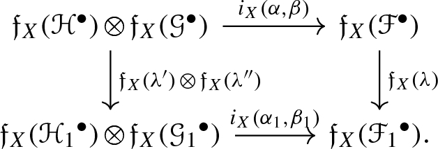
  such that the rows are short exact sequences, then the following diagram commutes:

  

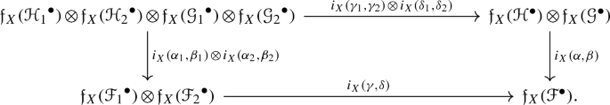
• (ii) Given a commutative diagram in $\mathbf{isVec} _b^\bullet (X)$,

  

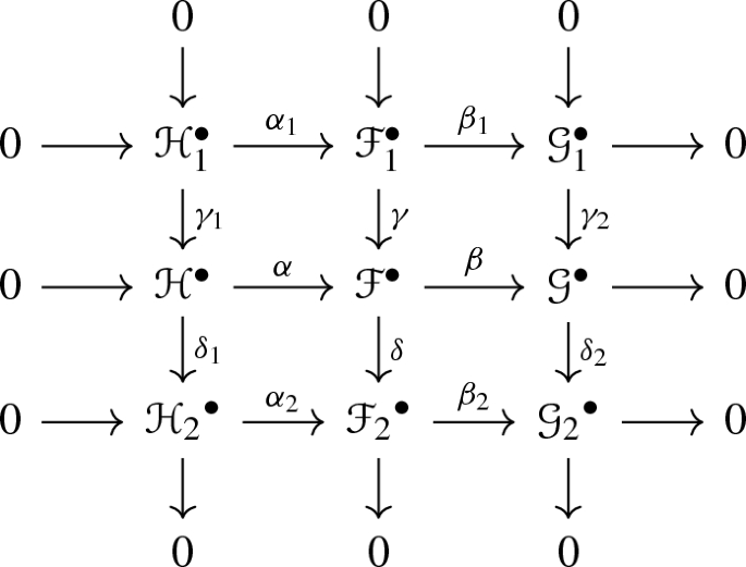
  such that rows and columns are short exact sequences, then the following diagram commutes:

  

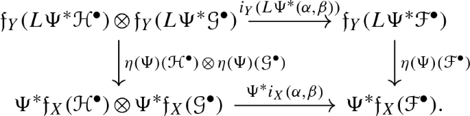
• (iii) ${\mathfrak {f}}_X$ and both commute with the base change of X. The explicit expression of such a property is the following: fix a morphism of schemes $\Psi :Y\rightarrow X$ and let $L\Psi ^*:\mathbf{D} _-(\mathbf{QCoh} (X))\rightarrow \mathbf{D} _-(\mathbf{QCoh} (Y))$ be the left derived functor of to the pullback $\Psi ^*$; then the following properties hold:

  • There is a natural transformation between functors: .

  • For any short exact sequence in $\mathbf{isVec} _b^\bullet (Y)$,

    

    the following diagram commutes:

    

• (iv) ${\mathfrak {f}}_X(0)=({\mathscr {O}}_X, 0)$. Moreover for the short exact sequence

  

  we have that is the canonical map (i.e., the “projection on the first component”).

• (v) If we canonically identify $\mathbf{isVec} (X)$ as a subcategory of $\mathbf{isVec} _b^\bullet (X)$, then ${\mathfrak {f}}_X$ restricts to and restricts to .

Theorem A.2

Up to natural transformation of functors there exists a unique determinant $({\mathfrak {f}}_X, i_X)$ on X. It will be denoted by $(\det _X, i_X)$.

Proof

See [13, Theorem 1] for a complete proof. Here we just write down the explicit expressions for $\det _X$:

The category is quite restrictive, for example it does not behave well with respect to the pushforward functor. Therefore, we would like to have a determinant functor for a more general category.

Definition A.3

A complex ${\mathscr {F}}^\bullet$ of ${\mathscr {O}}_X$-modules is said to be perfect if for any $x\in X$ there exist an open neighbourhood $U\ni x$, a complex ${\mathscr {G}}^\bullet$ in $\mathbf{Vec} ^\bullet _b(U)$ and a quasi-isomorphism of complexes of ${\mathscr {O}}_U$-modules . The category of perfect complexes on X is denoted by $\mathbf{Perf} (X)$, whereas $\mathbf{isPerf} (X)$ denotes the category of perfect complexes where the morphisms are just quasi-isomorphisms.

Theorem A.4

([13, Theorem 2]) The determinant $(\det _X,i_X)$ can be extended uniquely, up to natural transformation, to a determinant on . We will denote this extension again by the symbol $(\det _X,i_X)$ and formally it is the datum of:

• (1) A functor .

• (2) For any short exact sequence in ,

  

  an isomorphism

  

Moreover, properties (i)–(v) listed in Definition A.1 are satisfied in .

One of the most important applications of the determinant functor appears in arithmetic geometry if we consider its interaction with the usual pushfoward functor.

Definition A.5

Let $f:X\rightarrow S$ be a flat morphism between integral Noetherian schemes and let ${\mathscr {F}}$ be a coherent sheaf on X. It is well known [2, Exp. 3, Proposition 4.8] that the complex $Rf_*{\mathscr {F}}$ induced by the right derived functor of $f_*$ is a perfect complex on S. Then, just by composing $Rf_*$ with $\det _S$ it is possible to define the functor

which is called the determinant of cohomology (relative to f). Very often, for simplicity we want to forget about the graduation on the target of the determinant of cohomology, so it becomes a functor $\mathbf{isCoh} (X)\rightarrow \mathbf{Pic} (S)$.

Since the right derived functor $Rf_*$ is exact in the derived sense (see [11]) it is not hard to show that for any short exact sequence of coherent sheaves on X,

there is an isomorphism of graded invertible sheaves

Moreover, the whole construction behaves well with respect to flat base change in the following sense: assume that the following commutative square is given by a flat base change from S to $S'$:

then for any coherent sheaf ${\mathscr {F}}$ on X we have

$$\begin{aligned} g^*(\det Rf_*{\mathscr {F}})\cong \det Rf'_*(g'^*{\mathscr {F}}). \end{aligned}$$

(A.1)

We will also need an important property of the determinant of cohomology:

Proposition A.6

([13]) Let $f:X\rightarrow S$ be a flat morphism between integral Noetherian schemes and let ${\mathscr {F}}$ be a coherent sheaf on X. Moreover let ${\mathscr {L}}$ be an invertible sheaf on S. Then there is a canonical isomorphism between invertible sheaves on S,

where $X_s$ is a generic fibre of f.

Definition A.7

Let $\varphi :X\rightarrow S$ be a finite morphism between integral Noetherian schemes, then the norm of $\varphi$ is defined as the functor

B Original construction of Deligne pairing

In this section we give all details of the construction of the Deligne pairing described in [6].

S is a Dedekind scheme⁴ and we put . $\varphi :X\rightarrow S$ is an S-scheme satisfying the following properties:

• X is two-dimensional, integral, and regular. The generic point of X is $\eta$ and the function field of X is denoted by K(X).

• $\varphi$ is proper and flat.

• The generic fibre, denoted by $X_K$, is a geometrically integral, smooth, projective curve over K.

We say that X is an arithmetic surface over S.

In this section we will also need to recall the norm operator ${\mathcal {N}}$ in dimension 1 and 2 (it is formally different from the norm of an invertible sheaf defined above).

Definition B.1

Let C be a projective, non-singular curve over a field k, then for a closed point $x\in C$ and any non-zero rational function $f\in K(C)^{\times }$ such that $f\in {\mathscr {O}}^{\times }_{C,x}$ we put

(B.1)

where f(x) is the obvious element of k(x) associated to f. So if $D=\sum _{x\in C}n_x[x]\in {{\,\mathrm{Div}\,}}(C)$ and $f\in K(C)^{\times }$ is a non-zero rational function such that (f) and D have no common components, then the following element is well defined:

The well-known Weil reciprocity law says that

$$\begin{aligned} {\mathcal {N}}_{(g)}(f)={\mathcal {N}}_{(f)}(g). \end{aligned}$$

Coming back to our arithmetic surface $\varphi :X\rightarrow S$, consider

and note that if with $j=1,2$, then $(D_1+D_2,E_1+E_2)\in \Upsilon$.

Definition B.2

Let $(D,E)\in \Upsilon$ be such that D and E are both effective, then for any closed point $x\in X$ we put

This is called the local intersection number of D and E at x.

The local intersection number assigns the multiplicity of the intersection at each point of X, and the following basic result summarizes its naive properties.

Proposition B.3

Let $(E,D)\in \Upsilon$ and with $j=1,2$ be such that all the divisors are effective, then:

• (1) $i_x(D,E)=i_x(E,D)$.

• (2) .

• (3) $i_x(D,E)\ne 0$ if and only if .

• (4) If $x\in E$, $i_x(D,E)={{\,\mathrm{mult}\,}}_x(D|_E)$.

Proof

(1) and (3) are obvious. For (2) and (4) see [15, Lemma 9.1.4]. $\square$

Any divisor $D\in {{\,\mathrm{Div}\,}}(X)$ can be written in a unique way as $D=D_+-D_-$ where both $D_+$ and $D_-$ are effective and if $(D,E)\in \Upsilon$, then $(D_\pm ,E_\pm )\in \Upsilon$. We can use Definition B.2 in order to have the local intersection at x of D and E when (D, E) is any element of $\Upsilon$ (so not necessarily effective):

Definition B.4

Let (D, E) be an element of $\Upsilon$, then we define the 0-cycle on X given by

where [x] is a shorthand of $[\overline{\{x\}}].$

Remark B.5

The sum in Definition B.4 is finite because if D and E are effective without common components, then $i_x(D,E)={{\,\mathrm{mult}\,}}_x(D|_E)$ (Proposition B.3 (4)) and there is only a finite number of points on E at which the divisor $D|_E$ has non-zero multiplicity.

Proposition B.6

If with $j=1,2$, then the following properties hold for i(D, E):

• $i(D,E)=i(E,D)$ (symmetry).

• (bilinearity).

Proof

It follows immediately from Proposition B.3. $\square$

Definition B.7

We have the symmetric and bilinear pairing on $\Upsilon$:

$$\begin{aligned} \Upsilon&\rightarrow {{\,\mathrm{Div}\,}}(S)\\ (D,E)&\mapsto \langle D,E\rangle \end{aligned}$$

where

Let $\Gamma$ be a prime divisor of X with generic point $\gamma$ and consider a non-zero rational function $f\in K(X)^{\times }$ such that (f) and $\Gamma$ have no common components, then define ${\mathcal {N}}_{\Gamma }(f)\in K^{\times }$ in the following way:

where $N_{K(\Gamma )|K}$ is the usual field norm and $f|_{\Gamma }$ is defined as follows: since (f) and $\Gamma$ have no common components it follows that $v_{\gamma }(f)=0$, that is $f\in \mathscr {O}_{X,\gamma }^{\times }$. So $f|_{\Gamma }$ is the natural image of f in $k(\gamma )=K(\Gamma )$. At this point for any $D=\sum _i n_i\Gamma _i\in {{\,\mathrm{Div}\,}}(X)$ such that D and (f) have no common components we have

Since K(X) is the function field of any open subscheme $U\subseteq X$ and of $X_K$, we can restrict the operator to U and to $X_K$.

Proposition B.8

Let $f\in K(X)^{\times }$ and let be such that (f) and D have no common components, then the following claims hold:

• (1) Let $U\subseteq X$ be an open subscheme, then ${\mathcal {N}}_{D|_U}(f)={\mathcal {N}}_D(f)$.

• (2) ${\mathcal {N}}_{D|_{X_K}}(f)={\mathcal {N}}_D(f)$, where the left-hand side is the one-dimensional operator defined in equation (B.1).

Proof

In both items we can restrict to the case when $D=\Gamma$ is an irreducible horizontal divisor.

(1) The function fields and the generic points of $\Gamma$ and $\Gamma |_U$ coincide, so the claim follows trivially.

(2) Let $\gamma \in X_K$ be the generic point of $\Gamma$, it is a closed point of $X_K$ such that $k(\gamma )=K(\Gamma )$. By the bare definitions we can check the required equality. $\square$

Proposition B.9

([17, Proposition 4.3]) Let $f\in K(X)^{\times }$ and let $D\in {{\,\mathrm{Div}\,}}(X)$ be a divisor such that D and (f) have no common components, then

$$\begin{aligned}\langle D,(f)\rangle =({\mathcal {N}}_D(f))\in {{\,\mathrm{Princ}\,}}(S).\end{aligned}$$

Now we will construct the Deligne pairing and see the relation with the pairing $\langle D,E\rangle$ for divisors. We divide the construction in two steps:

Step 1. Definition of the K-vector space $\langle {\mathscr {L}},{\mathscr {M}}\rangle _K$.

Consider the sets

Note that $\Upsilon _K$ is just the set of couple of divisors with no common horizontal components. Now we define some vector spaces over K:

namely V is the free K-vector space over $\Sigma _K$.

(B.2)

(B.3)

Note that the above “” is the one-dimensional operator from Definition B.1 considered on the curve $X_K$.

Remark B.10

${\mathcal {N}}_{{{\,\mathrm{div}\,}}(m)|_{X_K}}(f)$ and $\mathcal N_{{{\,\mathrm{div}\,}}(l)|_{X_K}}(g)$ are well defined since (l, m), (fl, m), $(l,gm) \in \Sigma _K$, so ${{\,\mathrm{div}\,}}(m)|_{X_K}$ and (f) have no common components. The same holds for ${{\,\mathrm{div}\,}}(l)|_{X_K}$ and (g).

Define the free vector spaces and ; moreover put

which is considered as a constant sheaf (of K-vector spaces) over X. The natural image of any element $(l,m)\in \Sigma _K\subset V$ in $\langle {\mathscr {L}},{\mathscr {M}}\rangle _K$ is denoted by $\langle l,m\rangle _K$.

Proposition B.11

$\langle {\mathscr {L}},{\mathscr {M}}\rangle _K$ is a one-dimensional vector space over K.

Proof

Fix $(l_0,m_0)\in \Sigma _K$, then for any $(l,m)\in \Sigma _K$ there are two elements $f_0,g_0\in K(X)^{\times }$ such that $l=f_0l_0$, $m=g_0m_0$ and moreover,

By equations (B.2) and (B.3), in $\langle \mathscr {L},{\mathscr {M}}\rangle _K$ we can write

(B.4)

where, in order to simplify the notations, we put intended as operation on the curve $X_K$. This shows that $\langle {\mathscr {L}},{\mathscr {M}}\rangle _K$ has dimension at most 1 over K. Define the homomorphism of K-vector spaces

$$\begin{aligned} \theta :V\rightarrow K \end{aligned}$$

such that

Note that $\theta$ is non-trivial, so surjective, since $\theta (l_0,m_0)=1$. Now by using the Weil reciprocity law we prove that $\theta$ descends to a non-trivial morphism ${{\overline{\theta }}}:\langle {\mathscr {L}},{\mathscr {M}}\rangle _K\rightarrow K$, indeed for $f,g\in K(X)^{\times }$,

Similarly it holds that

In other words, equation (B.4) can we written as

hence, by the non-triviality of ${\overline{\theta }}$ we conclude that $\langle {\mathscr {L}},{\mathscr {M}}\rangle _K$ has dimension 1. $\square$

Step 2. Definition of $\langle {\mathscr {L}},{\mathscr {M}}\rangle$.

Let $U\subseteq S$ be a non-empty open subset and denote with $X_U$ the schematic inverse image of U with respect to $\varphi$. We clearly have a flat map $X_U\rightarrow U$, so we define

Moreover notice that $\Sigma _U\subset \Sigma _K$. We define a sheaf of ${\mathscr {O}}_S$-modules ${\mathscr {A}}$ on X given by

Finally consider the morphism of sheaves $\varPhi :\mathscr {A}\rightarrow \langle {\mathscr {L}},{\mathscr {M}}\rangle _K$ which sends $(l,m)\in \Sigma _U$ to $\langle l,m\rangle _K$ and define

The canonical image of $(l,m)\in \Sigma _U$ in ${\mathscr {A}}(U)$ is denoted as $\langle l,m \rangle _U$.

Proposition B.12

Let $(l,m)\in \Sigma _{U}$ be such that $\langle {{\,\mathrm{div}\,}}(l)|_{X_{U}}, {{\,\mathrm{div}\,}}(m)|_{X_{U}}\rangle =0\in {{\,\mathrm{Div}\,}}(U)$. Then for any there exists an element $a\in \mathscr {O}_S(U)$ such that .

Proof

There are two elements $f,g\in K(X)^{\times }$ such that , and moreover,

$$\begin{aligned}((f),(g)),\;((f),{{\,\mathrm{div}\,}}(m)),\;((g),{{\,\mathrm{div}\,}}(l))\in \Upsilon _K.\end{aligned}$$

Hence by using Proposition B.9,

Since $\langle {{\,\mathrm{div}\,}}(l')|_{X_{U}}, {{\,\mathrm{div}\,}}(m')|_{X_{U}}\rangle$ is effective,

On the other hand,

therefore by Proposition B.8 we can conclude that

$\square$

We are ready to show that $\langle {\mathscr {L}},{\mathscr {M}}\rangle$ is an invertible sheaf on S. By Proposition B.11, $\langle {\mathscr {L}},{\mathscr {M}}\rangle$ is non-zero; now assume $\mathscr {L}={\mathscr {O}}_X(D)$, ${\mathscr {M}}={\mathscr {O}}_X(E)$ and fix a point $s_0\in S$. By the moving lemma we can find a divisor $D'$ such that and $D'$ does not have components in $X_{s_0}$. Suppose that $x_1,\ldots , x_m$ are the intersection points of $D'$ and $X_{s_0}$, by applying again the moving lemma we can find a divisor $E'$ such that: , $E'$ and $D'+X_{s_0}$ have no common components, and E does not pass by $x_1,\ldots , x_m$. Consider the finite subset of S

and note that its complement has the following properties: $s_0\in U$ and $\langle D'|_U, E'|_U \rangle =0$. At this point any two meromorphic sections of ${\mathscr {L}}$ and ${\mathscr {M}}$ corresponding respectively to the divisors $D'$ and $E'$ will satisfy the hypothesis of Proposition B.12 on U. This implies that $\langle {\mathscr {L}},\mathscr {M}\rangle$ is an invertible sheaf.

One can show that the pairing constructed above satisfies axioms (1)–(4) of Definition 4.6 for $n=1$, moreover we have the following additional properties.

Theorem B.13

([17, Theorem 4.7]) The Deligne pairing $({\mathscr {L}},{\mathscr {M}})\rightarrow \langle \mathscr {L},{\mathscr {M}}\rangle$ satisfies the properties listed below. We assume that ${\mathscr {L}}$ and ${\mathscr {M}}$ are two invertible sheaves on X.

• (1) The induced map is bilinear and symmetric.

• (2) Let l and m be two non-zero meromorphic sections of ${\mathscr {L}}$ and ${\mathscr {M}}$, respectively, such that ${{\,\mathrm{div}\,}}(l)$ and ${{\,\mathrm{div}\,}}(m)$ have no common components. Then, there exists a non-zero meromorphic section $\langle l,m\rangle$ with the following properties:

  • (i) If $f,g\in K(X)^{\times }$ such that $({{\,\mathrm{div}\,}}(fl),{{\,\mathrm{div}\,}}(m)),({{\,\mathrm{div}\,}}(l),{{\,\mathrm{div}\,}}(gm))\in \Upsilon$, then

    

  • (ii) There is an isomorphism of invertible sheaves

    $$\begin{aligned} \langle {\mathscr {L}},{\mathscr {M}}\rangle \cong {\mathscr {O}}_S(\langle {{\,\mathrm{div}\,}}(l),{{\,\mathrm{div}\,}}(m)\rangle ). \end{aligned}$$

    Moreover, under the above isomorphism $\langle l,m\rangle$ corresponds to $1_{\langle {{\,\mathrm{div}\,}}(l),{{\,\mathrm{div}\,}}(m)\rangle }$. In particular,

    $$\begin{aligned} {{\,\mathrm{div}\,}}(\langle l,m\rangle )=\langle {{\,\mathrm{div}\,}}(l),{{\,\mathrm{div}\,}}(m)\rangle . \end{aligned}$$

Remark B.14

Note that when $S={{\,\mathrm{Spec}\,}}k$ for any field k (in other words X is an algebraic curve), then $\langle {\mathscr {L}},{\mathscr {M}}\rangle$ is just a one-dimensional k-vector space.

Remark B.15

If S is a non-singular projective curve over a field k, and $\varphi :X\rightarrow S$ is a morphism over ${{\,\mathrm{Spec}\,}}k$ (i.e., X is a fibred surface over S), then it is evident that satisfies all the axioms of Definition 3.1, so it is the intersection pairing on X. The same argument holds also when X has generic dimension n.

References

Beauville, A.: Complex Algebraic Surfaces. London Mathematical Society Student Texts, 2nd edn. Cambridge University Press, Cambridge (1996)
Berthelot, P., Grothendieck, A., Illusie, L. (directeurs): Théorie des intersections et théorème de Riemann–Roch. Lecture Notes in Mathematics. Springer, Berlin (1971)
Biswas, I., Schumacher, G., Weng, L.: Deligne pairing and determinant bundle. Electron. Res. Announc. Math. Sci. 18, 91–96 (2011)
Boucksom, S., Eriksson, D.: Spaces of norms, determinant of cohomology and Fekete points in non-Archimedean geometry. Adv. Math. 378, 107501 (2021)
Cartier, P.: Sur un théorème de snapper. Bull. Soc. Math. France 88, 333–343 (1960)
Deligne, P.: Le déterminant de la cohomologie. In: Ribet, K.A. (ed.) Current Trends in Arithmetical Algebraic Geometry. Contemporary Mathematics, vol. 67, pp. 93–177. American Mathematical Society, Providence (1987)
Ducrot, F.: Cube structures and intersection bundles. J. Pure Appl. Algebra 195(1), 33–73 (2005)
Elkik, R.: Fibrés d’intersections et intégrales de classes de Chern. Ann. Sci. École Norm. Sup. 22(2), 195–226 (1989)
Muñóz Garcia, E.: Fibrés d’intersection. Compositio Math. 124(3), 219–252 (2000)
Grothendieck, A.: Éléments de géométrie algébrique: IV. Étude locale des schémas et des morphismes de schémas IV. Inst. Hautes Études Sci. Publ. Math. 32, 5–361 (1967)
Hochenegger, A.: Appendix: Introduction to derived categories of coherent sheaves. Birational Geometry of Hypersurfaces, pp. 267–295 (2019). arXiv:1901.07305
Kleiman, S.L.: The Picard scheme. In: Schneps, L. (ed.) Alexandre Grothendieck: A Mathematical Portrait, pp. 35–74. International Press, Somerville (2014)
Knudsen, F.F., Mumford, D.: The projectivity of the moduli space of stable curves. I. Preliminaries on "det" and "Div". Math. Scand. 39(1), 19–55 (1976)
Kollár, J.: Rational Curves on Algebraic Varieties. Ergebnisse der Mathematik und ihrer Grenzgebiete. 3. Folge, vol. 32. Springer, Berlin (1996)
Liu, Q.: Algebraic Geometry and Arithmetic Curves. Oxford Graduate Texts in Mathematics. Oxford University Press, Oxford (2006)
Moret-Bailly, L.: Métriques permises. In: Seminar on Arithmetic Bundles: The Mordell Conjecture (Paris. 1983/84). Astérisque, vol. 127, pp. 29–87. Société Mathématique de France, Paris (1985)
Moriwaki, A.: Arakelov Geometry. Translations of Mathematical Monographs. American Mathematical Society, Providence (2014)
Phong, D.H., Ross, J., Sturm, J.: Deligne pairings and the Knudsen–Mumford expansion. J. Differential Geom. 78(3), 475–496 (2008)
Snapper, E.: Multiples of divisors. J. Math. Mech. 8, 967–992 (1959)
Snapper, E.: Polynomials associated with divisors. J. Math. Mech. 9, 123–139 (1960)
Xia, M.: Deligne–Riemann–Roch theorems I. Uniqueness of Deligne pairings and degree \(1\) part of Deligne–Riemann–Roch isomorphisms (2017). arXiv:1710.09731
Zhang, S.: Heights and reductions of semi-stable varieties. Compositio Math. 104(1), 77–105 (1996)
Acknowledgements
The author wants to express his gratitude to Robin S. De Jong for his time spent in discussing the topic during summer 2019 in Nottingham and for his precious insights. A special thanks goes also to Pietro Corvaja, Ivan Fesenko, Stefano Urbinati, Francesco Zucconi and to the anonymous referee for his/her careful reading and for providing thoughtful comments.
Funding
Open access funding provided by Universitá degli Studi di Udine within the CRUI-CARE Agreement.
Author information
Authors and Affiliations
Corresponding author
Additional information
Publisher's Note
Springer Nature remains neutral with regard to jurisdictional claims in published maps and institutional affiliations.
This research was supported by the Italian national grant “Ing. Giorgio Schirillo" conferred by INdAM and partially by the EPSRC programme grant EP/M024830/1 (Symmetries and Correspondences: Intra-Disciplinary Developments and Applications).