Compactifications of the moduli space of plane quartics and two lines

Abstract

We study the moduli space of triples $(C, L_1, L_2)$ consisting of quartic curves C and lines $L_1$ and $L_2$. Specifically, we construct and compactify the moduli space in two ways: via geometric invariant theory (GIT) and by using the period map of certain lattice polarized K3 surfaces. The GIT construction depends on two parameters $t_1$ and $t_2$ which correspond to the choice of a linearization. For $t_1=t_2=1$ we describe the GIT moduli explicitly and relate it to the construction via K3 surfaces.

Introduction

The construction of compact moduli spaces with geometric meanings is an important problem in algebraic geometry. In this article, we discuss the case of the moduli of K3 surfaces of degree 2 obtained as minimal resolutions of double covers of branched at a quartic C and two lines $L_1,L_2$, for which we give two constructions, one via Geometric Invariant Theory (GIT) for the plane curves $(C, L_1, L_2)$ depending on a choice of two parameters for each of the lines, and one via the period map of K3 surfaces. For a particular choice of parameters, we show that the constructions agree. Similar examples include [1, 2, 17, 18, 22, 23, 30]. Our interest on this example arose after the first two authors considered studying the variations of GIT quotients for a cubic surface and a hyperplane section [12]. The moduli of del Pezzo surfaces of degree 2 with two anti-canonical sections seems to be closely related to the moduli of K3 surfaces considered in this article, since del Pezzo surfaces of degree 2 with canonical singularities can be obtained as double-covers of branched at a (possibly singular) quartic curve. Also, a generic global Torelli for certain double covers of these K3 surfaces (namely, minimal resolutions of bi-double covers of along a quartic and four lines, cf. [14, Section 5.4.2]) can be derived using the results in this article and the methods in [28].

Following the general theory of variations of GIT quotients developed by Dolgachev and Hu [9] and independently by Thaddeus [32], we construct GIT compactifications for the moduli space of triples $(C, L_1, L_2)$ consisting of a smooth plane quartic curve C and two labeled lines $L_1,L_2$ in Sect. 2. These compactifications depend on parameters $t_1,t_2$ which are the ratio polarizations of the parameter spaces of quartic and linear homogeneous forms representing C and $L_1,L_2$. We generalize the study in [13] of GIT quotients of pairs (X, H) formed by a hypersurface X of degree d in and a hyperplane H to tuples $(X, H_1, \ldots , H_k)$ with several hyperplanes $H_i$, considering the relation between the moduli spaces of tuples with labeled and unlabeled hyperplanes. We then apply the setting to the case at hand, namely plane quartic curves and two lines. One sees in Lemma 2.9 that the space where the set of stable points is not empty can be precisely described. Furthermore, given a particular tuple, we can bound the set of parameters for which it is semistable (cf. Lemma 2.11).

Next we focus on the case when $t_1=t_2=1$. The moduli space can also be constructed via Hodge theory (cf. Sect. 3). The idea is to consider the K3 surface $S_{(C, L_1, L_2)}$ obtained by taking the desingularization of the double cover $\overline{S}_{(C,L_1,L_2)}$ of branched along the sextic curve $C+L_1+L_2$. Note that generically $\overline{S}_{(C,L_1,L_2)}$ admits nine ordinary double points (coming from the intersection points $C \cap L_1$, $C \cap L_2$ and $L_1 \cap L_2$). It follows that the K3 surface $S_{(C,L_1,L_2)}$ contains nine $(-2)$-curves which form a certain configuration. Call the saturated sublattice generated by these curves . Then the K3 surface $S_{(C,L_1,L_2)}$ is naturally M-polarized in the sense of Dolgachev [8]. Let be the locus where the sextic curves $C+L_1+L_2$ have at worst simple singularities (also known as ADE singularities or Du Val singularities). By associating to the triples $(C,L_1,L_2)$ the periods of the M-polarized K3 surfaces $S_{(C,L_1,L_2)}$ one obtains a period map from to a certain period domain . We shall prove that is an isomorphism.

Theorem 3.23

Consider the triples $(C, L_1, L_2)$ consisting of quartic curves C and lines $L_1,L_2$ such that $C + L_1 + L_2$ has at worst simple singularities. Let $S_{(C,L_1,L_2)}$ be the K3 surface obtained by taking the minimal resolution of the double plane branched along $C + L_1 +L_2$. The map sending $(C, L_1, L_2)$ to the periods of $S_{(C,L_1,L_2)}$ extends to an isomorphism .

The approach is analoguos to the one used by Laza [17]. Roughly speaking, we first consider the generic case where C is smooth and $C+L_1+L_2$ has simple normal crossings. Then we compute the (generic) Picard lattice M and the transcendental lattice $T = M_{\Lambda _{K3}}^{\perp }$ (see Proposition 3.13), determine the period domain and choose a suitable arithmetic group $\Gamma$ (cf. Sect. 3.3, N.B. $\Gamma$ is not the standard arithmetic group $O^*(T)$ used in [8] but an extension of $O^*(T)$). Finally we extend the construction to the non-generic case (using the methods and some results of [17]) and apply the global Torelli theorem and the surjectivity of the period map for K3 surfaces to prove the theorem (cf. Sects. 3.4 and 3.5).

Note that the period domain is a type IV Hermitian symmetric domain. The arithmetic quotients of admit canonical compactifications called Baily–Borel compactifications. To compare the GIT compactification and the Baily–Borel compactification we consider a slightly different moduli space (constructed by taking a quotient of the GIT quotient ) parameterizing triples $(C,L,L')$ consisting of quartic curves C and unlabeled lines $L,L'$. In a similar manner, we construct a period map and prove that is an isomorphism between the locus where $C+L+L'$ has at worst simple singularities and a certain locally symmetric domain (cf. Sect. 3.6). Moreover, we show in Corollary 2.16 that is the union of three points and five rational curves , whose incidence structure is describe in Fig. 1. The quasi-projective variety has codimension higher than 1 and hence the period map extends to the GIT compactification . Note also that preserves the natural polarizations (the polarization of is induced by the polarization of the moduli of plane sextics and the polarization of comes from the polarization of moduli of degree 2 K3 surfaces). A proof similar to [21, Theorem 7.6] shows that the extension of induces an isomorphism between the GIT quotient and the Baily–Borel compactification (see Sect. 3.7). Some computations and remarks on the Baily–Borel boundary components are also included in the paper (cf. Sect. 3.8).

Theorem 3.24

The period map extends to an isomorphism of projective varieties denotes the Baily–Borel compactification of .

Fig. 1

Incidence relations among the boundary components of the compactification of in . We denote $A \rightarrow B$ when the boundary component B is contained in the closure of the boundary component A

We conclude by the following remarks. The moduli space of quartic triples$(C,L_1,L_2)$ is closely related to the moduli space of degree 5 pairs (cf. [17, Definition 2.1]) consisting of a quintic curve and a line (i.e. given a triple $(C, L_1, L_2)$ that we consider, compare it with the pairs and ). Motivated by studying deformations of $N_{16}$ singularities, Laza [17] has constructed the moduli space of degree 5 pairs using both the GIT and Hodge theoretic approaches. His work is an important motivation for us and the prototype of what we do here. Also, the study of singularities and incidences lines on quartic curves is a classical topic (see for example the work of Edge [10, 11]) and a classifying space for such pairs may be related to our GIT compactification.

Variations of GIT quotients

In [13] the first two authors introduced a computational framework to construct all GIT quotients of pairs (X, H) formed by a hypersurface X of degree d and a hyperplane H in . They drew from the general theory of variations of GIT quotients developed by Dolgachev and Hu [9] and independently by Thaddeus [32]. The motivation was to construct compact moduli spaces of log pairs where X is Fano or Calabi–Yau. In this article we need to extend this setting to the case of tuples $(C,L_1,L_2)$ where C is a plane quartic curve and $L_1,L_2$ are lines. However, extending our work in [13] to two hyperplanes entails the same difficulties as for an arbitrary number of hyperplanes, while the dimension does not play an important role in the setting. Therefore we will consider the most general setting of a hypersurface in projective space and k hyperplane sections.

Variations of GIT quotients for n-dimensional hypersurfaces of degree d together with k (labeled) hyperplanes

Let be the parameter scheme of tuples $(F_d,l_1,\ldots ,l_k)$, where $F_d$ is a polynomial of degree d and $l_1,\ldots , l_k$ are linear forms in variables $(x_0,\ldots , x_{n+1})$, modulo scalar multiplication. We have

where $N= {\left( {\begin{array}{c}n+1+d\\ d\end{array}}\right) }-1$ and natural projections , for $i=1,\ldots , k$. The natural action of in extends to each of the factors in and therefore to itself. The set of G-linearizable line bundles is isomorphic to $\mathbb {Z}^{n+1}$. Then a line bundle is ample if and only if $a>0$, $b_i>0$ for $i=1,\ldots , k$, where

The latter is a trivial generalization of [13, Lemma 2.1]. Hence, for , the GIT quotient is defined as

where $t_i={b_i}/{a}$. Next, we explain why it is enough to consider the vector instead of $(a;b_1,\ldots , b_k)$. Let us introduce some notation.

Given a maximal torus , we can choose projective coordinates such that T is diagonal in G. Hence, any one-parameter subgroup is a diagonal matrix with diagonal entries $s^{r_i}$ where $r_i\in \mathbb Z$ for all i and . We say that $\lambda$ is normalized if $r_0\geqslant \cdots \geqslant r_{n+1}$ and $\lambda$ is not trivial. Any homogeneous polynomial g of degree d can be written as , where , , and . The support of g is . We have a natural pairing , which we use to introduce the Hilbert–Mumford function for homogeneous polynomials:

Define

which is piecewise linear on $\lambda$ for fixed $(f,l_1,\ldots ,l_k)$. Since the Hilbert–Mumford function is functorial [25, Definition 2.2, cf. p. 49], we can generalise [13, Lemma 2.2] to show that a tuple $(f,l_1,\ldots ,l_k)$ is (semi-)stable with respect to a polarisation if and only if

is negative (respectively, non-positive) for any normalized non-trivial one-parameter subgroup $\lambda$ of any maximal torus T of G. Hence the stability of a tuple is independent of the scaling of and as such, we may define:

Definition 2.1

Let $\vec t\in (\mathbb Q_{\geqslant 0})^k$. The tuple $(f,l_1,\ldots ,l_k)$ is $\vec t$ -stable (respectively $\vec t$ -semistable) if (respectively ) for all non-trivial normalized one-parameter subgroups $\lambda$ of G. A tuple $(f,l_1,\ldots ,l_k)$ is $\vec t$ -unstable if it is not $\vec t$-semistable. A tuple $(f,l_1,\ldots ,l_k)$ is strictly $\vec t$ -semistable if it is $\vec t$-semistable but not $\vec t$-stable.

Notice that the stability of a tuple $(f,l_1,\ldots ,l_k)$ is completely determined by the support of f and $l_1,\ldots ,l_k$. Moreover, notice that the $\vec t$-stability of a tuple is invariant under the action of G. Hence, we may say that a tuple $(X,H_1,\ldots , H_k)$ formed by a hypersurface and hyperplanes is $\vec t$ -stable (respectively, $\vec t$ -semistable) if some (and hence any) tuple of homogeneous polynomials $(f,l_1,\ldots ,l_k)$ defining $(X,H_1,\ldots ,H_k)$ is $\vec t$ -stable (respectively, $\vec t$ -semistable). A tuple $(X,H_1,\ldots , H_k)$ is $\vec t$ -unstable if it is not $\vec t$-semistable.

In [13], for fixed torus T in G, we introduced the fundamental set $S_{n,d}$ of one-parameter subgroups—a finite set—and we showed that if $k=1$ it was sufficient to consider the one-parameter subgroups in $S_{n,d}$ for each T to determine the $\vec t$-stability of any $(X,H_1)$. Let us recall the definition—slightly simplified from the original [13, Definition 3.1]—and extend the result to any k.

Definition 2.2

The fundamental set $S_{n,d}$ of one-parameter subgroups $\lambda \in T$ consists of all elements where

satisfying the following:

• such that for all $i=0,\ldots ,n+1$ and .

• .

• $(\gamma _0,\ldots ,\gamma _{n+1})$ is the unique solution of a consistent linear system given by n equations chosen from the following set:

  

The set $S_{n,d}$ is finite since there are a finite number of monomials of degree d in $n+2$ variables. Observe that $S_{n,d}$ is independent of the value of k. The following lemma is a straight forward generalization of [13, Lemma 3.2] which we include here for the convenience of the reader:

Lemma 2.3

A tuple $(X,H_1,\ldots ,H_k)$ given by equations $(f,l_1,\ldots ,l_k)$ is not $\vec t$-stable (respectively not $\vec t$-semistable) if and only if there is $g \in G$ satisfying

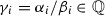
Moreover .

Proof

Let be the non-${\vec t}$-stable loci of with respect to a maximal torus T, and let be the non-$\vec t$-stable loci of .

By [7, p. 137], . Let $(f,l_1,\ldots ,l_k)$ be the equations in some coordinate system—inducing a maximal torus $T\subset G$—of a non-$\vec t$-stable tuple $(X,H_1,\ldots , H_k)$. Then, for some $\rho \in T'$ in a maximal torus $T'$ which may be different from T. All the maximal tori are conjugate to each other in G, and by [7, Exercise 9.2 (i)], we have for all $g\in G$. Hence, there is such that is normalized and satisfies. Normalized one-parameter subgroups in the coordinate system induced by T are the intersection of $\sum r_i=0$ and the convex hull of $r_i-r_{i+1}\geqslant 0$, where $i=0,\ldots , n$. The restriction of the $n+1$ linearly independent inequalities in $n+1$ variables to $\sum r_i=0$ gives a closed convex polyhedral subset $\Delta$ of dimension $n+1$ (in fact, a simplex) in the $\mathbb Q$-lattice of characters of T—isomorphic to the lattice of monomials (in variables $x_0,\ldots , x_{n+1}$) tensored by $\mathbb Q$, which in turn is isomorphic to $\mathbb Q^{n+2}$.

Given a fixed $(f,l_1,\ldots ,l_k)$, the function is piecewise linear and its critical points—the points in $\mathbb Q^{n+2}$ where fails to be linear—correspond to those monomials such that , or equivalently, the points such that for some . These points define a hyperplane in $\mathbb Q^{n+2}$ and the intersection of this hyperplane with $\Delta$ is a simplex of dimension n. As is linear on the complement of , the minimum of is achieved on the boundary, i.e. either on $\partial \Delta$ or on (for some $I,I'$), all of which are convex polytopes of dimension n. By finite induction, we conclude that the minimum of is achieved at one of the vertices of $\Delta$ or , which correspond precisely, up to multiplication by a constant, to the finite set of one-parameter subgroups in $S_{n,d}$. Indeed, observe that if is one such vertex, then for some where and . In addition, observe that we can find one such $\delta$ so that , thus giving the equations determining the maximal facets of $\Delta$, i.e. those where $r_i=r_{i+1}$. The lemma follows from the observation that .$\square$

Definition 2.4

The space of GIT stability conditions is

The space of GIT stability conditions is bounded, as it can be realized as a hyperplane section of . Since is a product of vector spaces (and hence a Mori dream space), is also a rational polyhedron. It is possible to precisely describe it and we will do this later for . Moreover, there is a finite number of non-isomorphic GIT compactifications as in varies. Therefore we have a natural division of into a finite number of disjoint rational polyhedrons of dimension k called chambers and the intersection of any two-chambers is a (possibly empty) rational polyhedron of smaller dimension which we will call a wall [9, Theorem 0.2.3]. The quotient is constant as $\vec t$ moves in the interior of a face or chamber. It is possible to find these walls explicitly by means of Lemma 2.3 (see [13, Theorem 1.1]) for given (n, d, k), since all walls of dimension $k-1$ should be a subset of the finite set of equations

(1)

Another interesting feature is that the the $\vec t$-stability of tuples $(X,H_1,\ldots , H_k)$ is equivalent of the t-stability of reducible GIT hypersurfaces of higher degree. Indeed:

Lemma 2.5

Let where for all $i=1,\ldots , k$. Let , such that and let . Let . A tuple $(X,H_1,\ldots ,H_k)$ is $\vec t$-(semi)stable if and only if the tuple

is $\vec {t'}$-(semi)stable.

In particular, if $t_1,\ldots , t_k$ are natural numbers, $(X,H_1,\ldots ,H_k)$ is $\vec t$-(semi)stable if and only if $X+{t_1}H_1+\cdots +{t_k}H_{k}$ (semi)stable in the classical GIT sense.

Proof

Let $\lambda$ be a normalized one-parameter subgroup, m be a positive integer and $g=\sum g_Ix^I$ be a homogeneous polynomial. Let J be such that

Then, since $\lambda$ is normalized, .

Let $(f,l_1,\ldots ,l_k)$ be the equations of $(X,H_1,\ldots , H_k)$ under some system of coordinates and let $\lambda$ be a normalized one-parameter subgroup. Using the above observation, the lemma follows from:

Corollary 2.6

Let and , $j\leqslant k$. Then a tuple $(X,H_1,\ldots , H_k)$ is $\vec t$-semistable if and only if is $\vec {t'}$-semistable.

Lemma 2.7

(cf. [12, Corollary 1.2]) If the locus of stable points is not empty, and $d \geqslant 3$, then

Proof

From [27, Theorem 2.1], any hypersurface where f is a homogeneous polynomial of degree $d\geqslant 3$ has . Hence, for any tuple $p=(X,H_1,\dots , H_K)$ such that X is smooth and $X\cap H_i$ has simple normal crossings, its stabilizer satisfies

where the last equality follows from [27, Theorem 2.1]. The result follows from [7, Corollary 6.2]:

Now let us consider the case of the symmetric polarization of . In order to do so, observe that the group $S_k$ acts on by defining the action of $h\in S_k$ as

$$\begin{aligned} h:(f,l_1,\ldots ,l_k)\mapsto (f,l_{h(1)},\ldots , l_{h(k)}). \end{aligned}$$

Define , which parametrizes classes of tuples $[(f,l_1,\ldots , l_k)]$ up to multiplication by a scalar and permutation of , i.e. for $g\in S_k$ and . Hence, we parameterize the same elements as in but we forget the ordering of the linear forms. In particular $\mathscr {R}'_{n,d,k}$ parametrizes pairs $[(X,H_1,\ldots , H_k)]$ formed by a hypersurface of degree d and k unordered hyperplanes. The quotient morphism is G-equivariant. Let such that $({b_1}/{a},\ldots ,{b_k}/{a})=(1,\ldots ,1)$ (i.e. we are considering $\vec t$-stability with respect to ). If the condition

(2)

holds, then a tuple $(f,l_1,\ldots , l_k)$ is $t_1$-(semi)stable if and only if is stable with respect to by [25, Theorem 1.1 and p. 48]. Hence, it is natural to define the GIT quotient

(3)

which is the GIT quotient of unordered tuples $(X,H_1,\cdots , H_k)$ with respect to the polarization . We have a commutative diagram

We want to determine all the orbits represented in from the orbits represented in via .

Choose $1\leqslant j_1< \cdots < j_l\leqslant k$ and define the G-equivariant morphism given by

By Lemma 2.5, we have a commutative diagram

Proposition 2.8

Let $1\leqslant j_1< \cdots <j_l\leqslant k$ and suppose that (2) holds. An unordered tuple $[(X,H_1,\dots ,H_k)]$—where X is a hypersurface of degree d in and $H_1,\ldots , H_k$ are k unordered hyperplanes—is (semi)stable with respect to if and only if

—a pair represented by a tuple in —is $\vec {t_*}$-(semi)stable. Moreover an orbit is closed if and only if and only if is closed. In addition, an orbit is closed if and only if is closed.

Proof

Since (2) holds, all the spaces in the above diagram are non-empty. As $\pi$ is finite, the pair $[(X,H_1,\dots ,H_k)]$—represented by the classes of tuples in —is (semi)stable with respect to if and only if every $(X,H_1, \dots ,H_k)$ in the class $[(X,H_1,\cdots ,H_k)]$ is $\vec t_*$-(semi)stable, by [25, Theorem 1.1 and p. 48]. By Lemma 2.5, $(X,H_1, \dots ,H_k)$—represented by tuples in —is $\vec t_*$-(semi)stable if and only if —represented by tuples in —is $\vec t_{*}$-(semi)stable (note that we use the notation $\vec t_*$ for vectors with all entries equal 1, whether $\vec t_*$ has k or $k-l$ entries). The last statement regarding closed orbits follows from noting that finite morphisms are closed, and hence is closed.$\square$

Symmetric GIT quotient of a quartic curve and two lines

We have seen how to construct GIT quotients for . In this section we apply our results to the case of quartic plane curves ($d=4$), but let us first show that our setting satisfies condition (2) for arbitrary degree. Hence, for the rest of the article, we assume that $n=1$ and $k=2$.

Lemma 2.9

The space of GIT stability conditions is

(4)

In particular, (2) holds.

Proof

Let be a vector and $(C,L_1,L_2)$ be a $\vec t$-semistable tuple. By choosing an appropriate change of coordinates, we may assume

Let . Then, as $t_1\geqslant 0, t_2\geqslant 0$, we have

Similarly, by taking a change of coordinates such that , , we may show that .

Recall that the space of GIT stability conditions is convex [9, 0.2.1]. Hence it is enough to show that all the vertices of the right hand side in (4) have a semistable tuple $(C, L_1,L_2)$ (and hence, they belong to ). These vertices correspond to the points (0, 0), (d / 2, 0), (0, d / 2) and (d, d). By Corollary 2.6, a tuple $(C, L_1,L_2)$ is (d / 2, 0)-semistable if and only if $(C, L_1)$ is (d / 2)-semistable, but the space of GIT t-stability conditions for plane curves and one hyperplane is [13, Theorem 1.1]. A mirrored argument applies for the stability point (0, d / 2).

Hence, we only need to exhibit a tuple $(C, L_1,L_2)$ which is (d, d)-semistable. Let . By Lemma 2.5, such a pair is t-semistable if and only if the reducible curve $C+dL_1+dL_2$ (defined by the equation $x_0^dx_1^dx_2^d=0$) of degree 3d is semistable in the usual GIT sense. The latter follows from the centroid criterion [13, Lemma 1.5].$\square$

There are two natural problems regarding the subdivision of into chambers and walls. One of them is to determine the walls and the solution is usually rather heavy computationally and geometrically speaking (see [12, 13] for the case $(n,d,k)=(2,3,1)$ and for a partial answer when $k=1$ and (n, d) are arbitrary). Given a tuple $(X, H_1,\cdots , H_k)$ the second problem consists on determining for which chambers and walls this tuple is (semi)stable. This problem may be easier to solve, especially when the answer to the first problem is known. The problem is simpler when $k=1$, as then is one-dimensional has a natural order. Nevertheless, we can give a partial answer when $n=1$, $k=2$ and d is arbitrary.

Definition 2.10

Let be the loci such that if and only $(C,L_1,L_2)$ is t-semistable.

Lemma 2.11

Suppose that C is a plane curve of degree d whose only singular point $p \in C$ is a linearly semi-quasihomogeneous singularity [17, Definition 2.21] with respect to the weights $\vec w=(w_1,w_2)$, $w_1 \geqslant w_2>0$. Suppose further that $C+L_1+L_2$ have simple normal crossings in . Let f be the localization of the equation of f at p and $\vec w(f)$ be its weighted degree with respect to $\vec w$.

• (a) Suppose that $p\not \in L_1\cup L_2$. Then

  

• (b) Suppose that $p\not \in L_2$ and $p\in L_1\cap C$. Then

  

Proof

We may choose a coordinate system such that is the singular point of C. We consider the one-parameter subgroup $\lambda = (2w_1-w_2, 2w_2-w_1,-w_1-w_2)$ which is normalized, as $w_1 \geqslant w_2$.

(a) The first statement is equivalent to show that if and then the triple is -unstable.

Let $l_1(x_0,x_1)+x_2$ and $l_2(x_0,x_1)+x_2$ be the equations of the lines $L_1$ and $L_2$, respectively, where $l_1,l_2$ are linear forms. We have

Therefore, $\mu _{t_1,t_2}(C,L_1, L_2, \lambda ) >0$ and the triple is destabilized by $\lambda$.

(b) The lines $L_1$ and $L_2$ have equation $l_1(x_0,x_1)$ and $l_2(x_0,x_1) +x_2$, respectively, where $l_1,l_2$ are linear forms. If , as $w_1\geqslant w_2$, we have

For the rest of the paper we consider tuples $(C, L_1, L_2)$ formed by a plane quartic C and two lines . The following result will come useful:

Lemma 2.12

(Shah [30, Section 2], cf. [19, Theorem 1.3]) Let Z be a plane sextic, and X the double cover of branched along Z. Then X has semi-log canonical singularities if and only if Z is semistable and the closure of the orbit of Z does not contain the orbit of the triple conic. In particular, a sextic plane curve with simple singularities is stable.

Lemma 2.13

Let $\vec t =(1,1)$ and $(C, L_1, L_2)$ be a tuple such that the sextic $C+L_1+L_2$ is reduced. Then, $(C, L_1, L_2)$ is $\vec t$-(semi)stable if and only if the double cover X of branched at $C+L_1+L_2$ has at worst simple singularities (respectively simple elliptic or cuspidal singularities).

Proof

The sextic (where f is a quartic curve and $l_1, l_2$ are distinct linear forms not in the support of f) cannot degenerate to a triple conic and it is reduced by hypothesis. By Lemma 2.12, Z is a GIT-semistable sextic curve if and only if X has slc singularities. The surface X is normal, as Z is reduced [6, Proposition 0.1.1]. In particular has hypersurface log canonical singularities away from the singular point , and by the classification of such singularities in [20, Table 1], they can only consist of either simple, simple elliptic or cuspidal singularities. If Z has only simple singularities then Z is GIT-stable by Lemma 2.12. Now suppose Z is GIT-stable and reduced. By [19, Theorem 1.3 and Remark 1.4] a GIT-semistable plane sextic curve has either simple singularities or it is in the open orbit of a sextic containing a double conic or a triple conic in its support, contradicting the fact that Z is reduced. Hence Z has only simple singularities. The proof follows from Lemma 2.5.$\square$

Remark 2.14

Although, we will not discuss other polarizations. It is worth to notice that for $\vec t=( \epsilon , \epsilon )$ the stability is very similar to the one of plane quartics. In particular, if C is a semistable quartic and $L_1,L_2$ are lines in general position. Then, the triple $(C, L_1, L_2)$ is stable.

Let and be the set of $\vec t$-stable and $\vec t$-semistable tuples $(f,l_1,l_2)$, respectively. Let

Let $\vec t=(1,1)$. By Lemma 2.12, . Let , and recall that . Then . We are interested in describing the compactification of by . We use the notation in [19].

Lemma 2.15

The quotient is the compactification of by three points and six rational curves. The three points correspond to the closed orbit of tuples $(C,L_1,L_2)$ defined up to projective equivalence by the following tuples:

The six rational curves correspond to the closed orbit of tuples $(C,L_1,L_2)$ defined up to projective equivalence by the following cases:

where $a \ne 0,1, \infty$.

Proof

Let , parametrising tuples $(g,l_1)$ up to multiplication by scalar where g is a quintic homogeneous polynomial and $l_1$ is a linear form. As we have seen in Proposition 2.8, we have a morphism defined by , and an orbit O of is closed if and only if the orbit $\phi _2(O)$ of is closed.

Hence the points which compactify into corresponding to closed orbits of are mapped via $\phi _2$ onto points in corresponding to closed orbits in . Hence we just need to identify closed orbits in . Our result is a straight forward identification of these orbits in the classification of in [17, Proposition 3.22] (Fig. 2).$\square$

Fig. 2

Triples parametrized by . The dotted and dashed lines represent the lines $L_1$ and $L_2$, respectively (see Lemma 2.15)

Lemma 2.15, together with Proposition 2.8 gives us the following compactification which will be of interest for the next section:

Corollary 2.16

Let be the GIT compactification of a quartic plane curve and two unlabeled lines and let be the open loci parametrizing triples $(C,L,L')$ such that $C+L+L'$ is reduced and has at worst simple singularities. Then, is the union of three points, , , and five rational curves, , , , , , which are obtained as images—via the natural morphism —of points and rational curves described in Lemma 2.15, as follows:

• the points are the images of the points , and

• the rational curves , are the images of the rational curves .

Moreover, the boundary components and in are mapped onto the same boundary component in .

Moduli of quartic plane curves and two lines via K3 surfaces

On K3 surfaces and lattices

By a lattice we mean a finite dimensional free $\mathbb {Z}$-module L together with a symmetric bilinear form $(-,-)$. The basic invariants of a lattice are its rank and signature. A lattice is even if $(x,x) \in 2\mathbb {Z}$ for every $x \in L$. The direct sum of two lattices $L_1$ and $L_2$ is always assumed to be orthogonal, which will be denoted by . For a lattice $M \subset L$, $M_L^{\perp }$ denotes the orthogonal complement of M in L. Given two lattices L and $L'$ and a lattice embedding $L \hookrightarrow L'$, we call it a primitive embedding if is torsion free.

We shall use the following lattices: the (negative definite) root lattices $A_n$ ($n \geqslant 1$), $D_m$ ($m \geqslant 4$), $E_r$ ($r = 6,7,8$) and the hyperbolic plane U. Given a lattice L, L(n) denotes the lattice with the same underlying $\mathbb {Z}$-module as L but with the bilinear form multiplied by n.

Notation 3.1

Given any even lattice L, we define:

• , the dual lattice;

• , the discriminant group endowed with the induced quadratic form ;

• : the determinant of the Gram matrix (i.e. the intersection matrix) with respect to an arbitrary $\mathbb {Z}$-basis of L;

• O(L): the group of isometries of L;

• $O(q_L)$: the automorphisms of $A_L$ that preserve the quadratic form $q_L$;

• $O_{-}(L)$: the group of isometries of L of spinor norm 1 (see [29, Section 3.6]);

• $\widetilde{O}(L)$: the group of isometries of L that induce the identity on $A_L$;

• $O^*(L) = O_{-}(L) \cap \widetilde{O}(L)$;

• $\Delta (L)$: the set of roots of L ($\delta \in L$ is a root if );

• W(L): the Weyl group, i.e. the group of isometries generated by reflections $s_{\delta }$ in root $\delta$, where .

For a surface X, the intersection form gives a natural lattice structure on the torsion-free part of $H^2(X, \mathbb {Z})$ and on the Néron–Severi group . For a K3 surface S, we have , and hence . Both $H^2(S, \mathbb {Z})$ and are torsion-free and the natural map is a primitive embedding. Given any K3 surface S, $H^2(S,\mathbb {Z})$ is isomorphic to , the unique even unimodular lattice of signature (3, 19). We shall use $O(S),\Delta (S),W(S)$, etc. to denote the corresponding objects of the lattice . We also denote by $\Delta ^+(S)$ and $V^+(S)$ the set of effective $(-2)$ divisor classes in and the Kähler cone of S respectively.

In our context, a polarization for a K3 surface is the class of a nef and big divisor H (and not the most restrictive notion of ample divisor, we follow the terminology in [17]) and $H^2$ is its degree. More generally there is a notion of lattice polarization. We shall consider the period map for (lattice) polarized K3 surfaces and use the standard facts on K3 surfaces: the global Torelli theorem and the surjectivity of the period map. We also need the following theorem (see [24, p. 40] or [17, Theorem 4.8, Proposition 4.9]).

Theorem 3.2

Let H be a nef and big divisor on a K3 surface S. The linear system |H| has base points if and only if there exists a divisor D such that and $D^2=0$.

The K3 surfaces associated to a generic triple

We first consider the K3 surfaces arising as a double cover of branched at a smooth quartic curve C and two different lines $L_1$ and $L_2$ such that $C+L_1+L_2$ has simple normal crossings. We shall show that these K3 surfaces are naturally polarized by a certain lattice.

Denote by $\overline{S}_{(C,L_1,L_2)}$ the double cover of branched along $C+L_1+L_2$. Let $S_{(C,L_1,L_2)}$ be the K3 surface obtained as the minimal resolution of the nine singular points of $\overline{S}_{(C,L_1,L_2)}$. Let be the natural morphism. Note that also factors as the composition of the blow-up of at the singularities of $C+L_1+L_2$ and the double cover of the blow-up branched along the strict transforms of C, $L_1$ and $L_2$ (see [4, Section III.7]).

Let be the pullback of the class of a line in . The class h is a degree 2 polarization of $S_{(C,L_1,L_2)}$. We assume that $C \cap L_1 = \{p_1, p_2, p_3, p_4\}$, and . Denote the classes of the exceptional divisors corresponding to $p_i$, $q_i$, and r by $\alpha _i$, $\beta _i$ and $\gamma$ respectively ($1 \leqslant i \leqslant 4$). Let us also denote by $l_1'$ (respectively $l_2'$) the class of the strict transform of $L_1$ (respectively $L_2$). Note that the morphism is given by the class

(5)

It is straightforward to check that , , for $1 \leqslant i,j \leqslant 4$. Clearly, we have , , and for $1 \leqslant i,j \leqslant 4$.

Consider the sublattice of the Picard lattice of $S_{(C,L_1,L_2)}$ generated by the curve classes $\gamma ,l_1',\alpha _1, \ldots , \alpha _4,l_2',\beta _1, \ldots , \beta _4$. Let

It follows from (5) that forms a $\mathbb {Z}$-basis of the sublattice. The Gram matrix with respect to this basis is computed as follows:

$$\begin{aligned} \left( {\begin{array}{c@{\quad }c@{\quad }c@{\quad }c@{\quad }c@{\quad }c@{\quad }c@{\quad }c@{\quad }c@{\quad }c} -2 &{} 1 &{} 0 &{} 0 &{} 0 &{} 1 &{} 0 &{} 0 &{} 0 &{} 2 \\ 1 &{} -2 &{} 1 &{} 1 &{} 1 &{} 0 &{} 0 &{} 0 &{} 0 &{} 0 \\ 0 &{} 1 &{} -2 &{} 0 &{} 0 &{} 0 &{} 0 &{} 0 &{} 0 &{} 0 \\ 0 &{} 1 &{} 0 &{} -2 &{} 0 &{} 0 &{} 0 &{} 0 &{} 0 &{} 0 \\ 0 &{} 1 &{} 0 &{} 0 &{} -2 &{} 0 &{} 0 &{} 0 &{} 0 &{} 0 \\ 1 &{} 0 &{} 0 &{} 0 &{} 0 &{} -2 &{} 1 &{} 1 &{} 1 &{} 0 \\ 0 &{} 0 &{} 0 &{} 0 &{} 0 &{} 1 &{} -2 &{} 0 &{} 0 &{} 0 \\ 0 &{} 0 &{} 0 &{} 0 &{} 0 &{} 1 &{} 0 &{} -2 &{} 0 &{} 0 \\ 0 &{} 0 &{} 0 &{} 0 &{} 0 &{} 1 &{} 0 &{} 0 &{} -2 &{} 0 \\ 2 &{} 0 &{} 0 &{} 0 &{} 0 &{} 0 &{} 0 &{} 0 &{} 0 &{} 0 \\ \end{array} } \right) _{\textstyle .} \end{aligned}$$

Notation 3.3

Let M be the abstract lattice of rank 10 spanned by an ordered basis

with the intersection form given by the above Gram matrix, which we will call $G_M$. Notice that M is an even lattice. If $S_{(C,L_1,L_2)}$ is a K3 surface obtained as above from a smooth quartic C and two lines $L_1,L_2$ such that $C+L_1+L_2$ has simple normal crossings, then there is a natural lattice embedding as described before.

We set $h = \gamma + \xi$. Observe that $\jmath (h)$ is linearly equivalent to the pullback of a line in via $\pi$ and therefore, it is a base point free polarization. In particular, we have $(h,h) = 2$, $(h,l_1') = (h, l_2') = 1$, and for . We also let and .

Let us compute the discriminant group $A_M$ and the quadratic form .

Lemma 3.4

The discriminant group is isomorphic to $(\mathbb {Z}/2\mathbb {Z})^{\oplus 6}$.

Proof

Let us denote by (respectively ) the dual element of $\alpha _i\in M$ (respectively , for $1 \leqslant i,j \leqslant 3$). Recall that $\alpha _i^*$ is defined to be the unique element of $M^*$ such that $(\alpha _i^*, \alpha _i) = 1$ and the pairing of $\alpha _i^*$ with any other element of the basis is 0. We define and $\xi ^*$ in a similar way. The coefficients of the dual elements $\gamma ^*\!, l_1'^*, \alpha _1^*, \alpha _2^*, \alpha _3^*, l_2'^*, \beta _1^*, \beta _2^*, \beta _3^*, \xi ^*$ (with respect to the basis ) can be read from the rows or columns of the inverse matrix $G_M^{-1}$ of the Gram matrix $G_M$ of M:

$$\begin{aligned} G_M^{-1}= \left( {\begin{array}{c@{\quad }c@{\quad }c@{\quad }c@{\quad }c@{\quad }c@{\quad }c@{\quad }c@{\quad }c@{\quad }c} 0 &{} 0 &{} 0 &{} 0 &{} 0 &{} 0 &{} 0 &{} 0 &{} 0 &{} \frac{1}{2} \\ 0 &{} -2 &{} -1 &{} -1 &{} -1 &{} 0 &{} 0 &{} 0 &{} 0 &{} 1 \\ 0 &{} -1 &{} -1 &{} -\frac{1}{2} &{} -\frac{1}{2} &{} 0 &{} 0 &{} 0 &{} 0 &{} \frac{1}{2} \\ 0 &{} -1 &{} -\frac{1}{2} &{} -1 &{} -\frac{1}{2} &{} 0 &{} 0 &{} 0 &{} 0 &{} \frac{1}{2} \\ 0 &{} -1 &{} -\frac{1}{2} &{} -\frac{1}{2} &{} -1 &{} 0 &{} 0 &{} 0 &{} 0 &{} \frac{1}{2} \\ 0 &{} 0 &{} 0 &{} 0 &{} 0 &{} -2 &{} -1 &{} -1 &{} -1 &{} 1 \\ 0 &{} 0 &{} 0 &{} 0 &{} 0 &{} -1 &{} -1 &{} -\frac{1}{2} &{} -\frac{1}{2} &{} \frac{1}{2} \\ 0 &{} 0 &{} 0 &{} 0 &{} 0 &{} -1 &{} -\frac{1}{2} &{} -1 &{} -\frac{1}{2} &{} \frac{1}{2} \\ 0 &{} 0 &{} 0 &{} 0 &{} 0 &{} -1 &{} -\frac{1}{2} &{} -\frac{1}{2} &{} -1 &{} \frac{1}{2} \\ \frac{1}{2} &{} 1 &{} \frac{1}{2} &{} \frac{1}{2} &{} \frac{1}{2} &{} 1 &{} \frac{1}{2} &{} \frac{1}{2} &{} \frac{1}{2} &{} -\frac{1}{2} \end{array} } \right) _{\textstyle .} \end{aligned}$$

For instance, , where we identify each element of M with its image in $M^*$. By abuse of notation, we also use to denote the corresponding elements in . Observe that $l_1'^* = l_2'^* \equiv 0 \in A_M$. It is straightforward to verify that $A_M$ can be generated by and hence $A_M$ is isomorphic to $(\mathbb {Z}/2\mathbb {Z})^{ \oplus 6}$. Indeed, this follows from observing from the columns of $G_M^{-1}$ that $\alpha ^*_3=\gamma ^* + \alpha _1^*+\alpha _2^*\in A_M$ and $\beta ^*_3=\gamma ^* + \beta _1^*+\beta _2^*\in A_M$.$\square$

Remark 3.5

We derive a formula for the quadratic form $q_M:A_M \rightarrow \mathbb {Q}/2\mathbb {Z}$:

$$\begin{aligned}&q_M\bigl (a\gamma ^* + b\alpha _1^* + c\alpha _2^* + d\beta _1^* + e\beta _2^* + f\xi ^*\bigr )\\ {}&\;\;\equiv b^2 + c^2 +bc + d^2 + e^2 + de + (a+b+c+d+e)f - \frac{1}{2}\, f^2 \in \mathbb {Q}/2\mathbb {Z}. \end{aligned}$$

Proposition 3.6

Let S be a K3 surface. If is a lattice embedding such that $\jmath (h)$ is a base point free polarization and , and ($1 \leqslant i,j \leqslant 3$) all represent irreducible curves, then $\jmath$ is a primitive embedding.

Proof

Assume that $\jmath$ is not primitive. Then the embedding $\jmath$ must factor through the saturation of M which is a non-trivial even overlattice of M: . By [26, Proposition 1.4.1], there is a bijection between even overlattices of M and isotropic subgroups of (which are generated by isotropic elements, i.e. $v\in A_M$ such that $q_M(v)=0$). Using Lemma 3.4 and Remark 3.5, it is easy to classify the isotropic elements of $A_M$. As and in $A_M$, there are only three cases to consider. We drop the embedding $\jmath$ in the rest of the proof.

Case 1. The isotropic element is $\gamma ^*$. From the columns of $G_M^{-1}$ we see that $\gamma ^* = \xi /2 \in A_M$. Hence, we have $\xi = 2x$ for some . But then and which would imply that h is not base point free by Theorem 3.2.

Case 2. The isotropic element is where $1 \leqslant i,j \leqslant 3$. Let us take $\alpha _1^* + \beta _1^*$ for example. The other cases are similar. Note that in $A_M$. We have $\alpha _2 + \alpha _3 + \beta _2 + \beta _3 = 2y$ for some . Because S is a K3 surface and , either y or $-y$ is effective. Note that $l_1'$, $l_2'$, $\alpha _i$ and ($1 \leqslant i,j \leqslant 3$) are irreducible curves (by the assumption), h is nef and . It follows that is nef. Since , y is effective. Because $(y,\alpha _2) = (y, \alpha _3) = (y, \beta _2) = (y, \beta _3) = -1$, we know $\alpha _2,\alpha _3,\beta _2$ and $\beta _3$ are in the support of y. Write $y = m\alpha _2 + n\alpha _3 + k \beta _2 + l \beta _3 + D = (\alpha _2 + \alpha _3 + \beta _2 + \beta _3)/2$ where D is an effective divisor, and $m,n,k,l \geqslant 1$. But then we have a contradiction

Case 3. The isotropic element is where $1 \leqslant i,j \leqslant 3$. Take $\alpha _1^* + \beta _1^* + \gamma ^*$ for example. Since $\alpha _1^* + \beta _1^* + \gamma ^* = \alpha _2 /2+ \alpha _3/2 + \beta _2/2 + \beta _3/2 + \xi /2$ in $A_M$, there exists an element z of such that . Because S is a K3 surface, and $(z,h) = 1$, the class z represents an effective divisor. By the assumption $l_1',l_2',\alpha _i$ and ($1 \leqslant i,j \leqslant 3$) represent irreducible curves. Note that . Let us write $z = m\alpha _2 + n\alpha _3 + k\beta _2 + l\beta _3 + D$, where D is effective, and $m,n,k,l > 0$. Then we have

which implies that $(D, l_1') < 0$ and $(D, l_2') < 0$. Now we write

$$\begin{aligned} z = m\alpha _2 + n\alpha _3 + k\beta _2 + l\beta _3 + sl_1' + tl_2'+D' \end{aligned}$$

where $D'$ is effective, and $m,n,k,l,s,t \geqslant 1$. But this is impossible: $2\leqslant s+t \leqslant (z, h) = 1$. $\square$

Corollary 3.7

Let C be a smooth plane quartic curve and $L_1$, $L_2$ two distinct lines such that $C+L_1+L_2$ has simple normal crossings and let be the lattice embedding given in Notation 3.3. Then $\jmath$ is a primitive embedding.

The proof of Proposition 3.6 can easily be adapted to proof the following lemma.

Lemma 3.8

Let S be a K3 surface and be a lattice embedding. If none of $\jmath (\xi )$, or ($1 \leqslant i, i'\!, j, j' \leqslant 3$) is divisible by 2 in , then the embedding $\jmath$ is primitive.

Proposition 3.9

Assume that S is a K3 surface such that is isomorphic to the lattice M. Then S is the double cover of branched over a reducible curve $C + L_1 + L_2$ where C is a smooth plane quartic, $L_1, L_2$ are lines and $C+L_1+L_2$ has simple normal crossings.

Proof

By assumption there exist satisfying the numerical conditions in Notation 3.3. Without loss of generality, we assume that h is nef (this can be achieved by acting by $\pm W(S)$). Then $l_1'$ and $l_2'$ are both effective (as , $(h,l_i')=1$). We further assume that ($1 \leqslant i,j \leqslant 4$) and $\gamma$ are effective (apply $s_{\alpha _i}$ or or $s_{\gamma }$ if necessary).

As h is nef and $(h,h)=2>0$, h is a polarization of degree 2. We will show that h is base point free by reductio ad absurdum. By Theorem 3.2, there exists a divisor D such that $(D, D) = 0$ and $(h, D) = 1$. Note that this is a numerical condition. Write D as a linear combination of $\gamma , l_1', \alpha _1, \ldots , \alpha _3, l_2', \beta _1, \ldots , \beta _3$ and $\xi$, with coefficients $c_1,\ldots , c_{10}$. Let $S_{(Q,L,L')}$ be the K3 surface associated to a smooth quartic curve Q and two lines $L,L'$ such that $Q+L+L'$ has simple normal crossings. Find the curve classes corresponding to $\gamma , l_1', \alpha _1, \ldots , \alpha _3, l_2', \beta _1, \ldots , \beta _3,\xi$ (as what we did at the beginning of this subsection) and consider their linear combination $D'$ with coefficients $c_1,\ldots , c_{10}$, the same values as in the expression for D. Then, both D and $D'$ satisfy the same numerical conditions in S (respectively $S_{(Q,L,L')}$) with respect to the divisor class $h= \gamma + \xi$. Again, by Theorem 3.2 the pull-back h of in $S_{(Q,L,L')}$ has base points, which gives a contradiction. So the linear system of h defines a degree two map . Since S is a K3 surface of degree 2, the branching locus must be a sextic curve B.

Consider . Note that $(h'\!, h')>0$ and $(h'\!, h) > 0$. We can write any effective divisor as

(6)

where $a_i, b_i, c\in \mathbb Z$, where $0\leqslant i\leqslant 4$. Let $k_i= a_0/2-a_i$, $l_i= b_0/2-b_i$ where $1\leqslant i\leqslant 4$. It follows that

(7)

Let $D\in \Delta (S)$ as in (6). Then implies that

(8)

First note that when $a_0+b_0=(D,h)=0$, then (8) gives that either and or $c=0$, and all coefficients in but one equal 0 and . In particular, . If $D\in \Delta ^+(S)\cap \langle h \rangle ^{\perp }_M$, then $(D,h)=a_0+b_0=0$ which in turn implies that .

Now suppose that $D\in \Delta ^+(S)$ and $(h,D)>0$. Then (7) implies that $a_0+b_0>0$ and (8) gives $c\geqslant 0$. Then, by the arithmetic-geometric mean inequality and (8), we get

where the latter inequality follows from observing that the first summand is positive and

Hence $(h'\!,D)>0$ for all $D\in \Delta ^+(S)$. Moreover, if $D \subset S$ is rational and $D \not \in \Delta ^+(S)$, then $\pi _*(D)\ne 0$ and . Hence, by [15, Corollary 8.1.7], $h'$ is ample.

Because $(h'\!, l_1')=1$, the class $l_1'$ is represented by an irreducible curve. Similarly, $l_2',\alpha _i$ and ($1 \leqslant i,j \leqslant 3$) all correspond to irreducible curves. It follows that the irreducible rational curves $\alpha _1, \ldots , \alpha _4, \beta _1, \ldots , \beta _4$ are contracted by $\pi$ to ordinary double points of the sextic B. Let $L_1'$ (respectively $L_2'$) be the unique irreducible curve in S corresponding to the class $l_1'$ (respectively $l_2'$) and set $L_1 = \pi (L_1')$ (respectively $L_2 = \pi (L_2')$). Since , the projection formula implies that $L_1$ is a line. Moreover, the line $L_1$ has to pass through four ordinary double points of the branched curve B since . Similarly, $L_2$ is also a line passing through four different ordinary double points of B. (Note that both $L_1$ and $L_2$ pass through the singularity of B corresponding to $\gamma$.) By Bezout’s theorem, the two lines $L_1$ and $L_2$ are both components of B (otherwise we have contradictions: and analogously for $L_2$).$\square$

Corollary 3.10

For a sufficiently general triple $(C, L_1, L_2)$ (i.e. outside the union of a countable number of proper subvarieties of the moduli space), the Picard lattice coincides with M via the embedding $\jmath$.

Proof

The argument in [16, Corollary 6.19] works here. Alternatively, let $L_1$ and $L_2$ be given by linear forms $l_1$ and $l_2$, respectively, and consider the elliptic fibration defined by the function . If $(C, L_1, L_2)$ is sufficiently general, then the pencil of lines generated by $L_1$ and $L_2$ only consists of lines intersecting C normally or lines tangent to C at a point. As a result, the elliptic fibration contains two reducible singular fibers of type $I_0^*$ (i.e. with 5 components) and 12 singular fibers of type $I_1$ (i.e. with one nodal component), where we follow Kodaira’s notation as in [4, Section V.7], [15, Section 11.1.3]. Note that the fibration admits a 2-section $\gamma$. Consider the associated Jacobian fibration (see for example [15, Section 11.4]). By the Shioda–Tate formula [15, Corollaries 11.3.4 and 11.4.7], the K3 surface $S_{(C,L_1,L_2)}$ has Picard number 10 which equals the rank of M. Moreover, we have [15, Section 11, (4.5)]:

It is easy to compute that the Gram matrix $G_M$ has determinant $(-64)$. The proposition then follows from the following standard fact on lattices (which implies):

As and they have the same rank and discriminant, then .$\square$

Now let us consider the case when C has at worst simple singularities not contained in $L_1+L_2$ and $C+L_1+L_2$ has simple normal crossings away from the singularities of C. We still use $S_{(C,L_1,L_2)}$ to denote the K3 surface obtained as a minimal resolution of the double cover of along $C+L_1+L_2$. The rank 10 lattice M is the same as in Notation 3.3.

Lemma 3.11

If C has at worst simple singularities not contained in $L_1+L_2$ and $C+L_1+L_2$ has simple normal crossings away from the singularities of C, then there exists a primitive embedding such that $\jmath (h)$ is a base point free degree two polarization.

Proof

Thanks to the transversal intersection, we define the embedding $\jmath$ as in the generic case. In particular, the morphism is defined by $\jmath (h)$. The embedding $\jmath$ is primitive by Proposition 3.6.$\square$

M-polarized K3 surfaces and the period map

In this subsection let us compute the (generic) Picard lattice M and the transcendental lattice T. Then we shall determine the period domain and define a period map for generic triples $(C, L_1, L_2)$ via the periods of M-polarized K3 surfaces $S_{(C, L_1, L_2)}$.

Definition 3.12

Let M be the lattice defined in Notation 3.3. An M -polarized K3 surface is a pair $(S, \jmath )$ such that is a primitive lattice embedding. The embedding $\jmath$ is called the M -polarization of S. We will simply say that S is an M -polarized K3 surface when no confusion about $\jmath$ is likely.

We now determine the lattice M and show that it admits a unique primitive embedding into the K3 lattice $\Lambda _{K3}$.

Proposition 3.13

Let M be the lattice defined in Notation 3.3. Then M is isomorphic to the lattice $U(2) \perp A_1^{2} \perp D_6$ and admits a unique primitive embedding (up to isometry) $M \hookrightarrow \Lambda _{K3}$ into the K3 lattice $\Lambda _{K3}$. The orthogonal complement with respect to the embedding is isometric to $U \perp U(2) \perp A_1^{2} \perp D_6$.

Proof

By [26, Corollary 1.13.3] the lattice M is uniquely determined by its invariants which can be easily computed from the Gram matrix $G_M$ (see also Lemma 3.4 and Remark 3.5).

• M has rank 10 and signature (1, 9).

• The Gram matrix $G_M$ has determinant $(-64)$.

• The discriminant group is 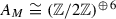with quadratic form , where $u,w_{2,1}^{1}$ and $w_{2,1}^{-1}$ are the discriminant forms associated to $U(2),E_7$ and $A_1$ respectively (cf. [5, Section 1.5 and Appendix A] and references therein). Note that is isomorphic to the discriminant form of $D_6$.

By [26, Theorem 1.14.4] the lattice M admits a unique primitive embedding into $\Lambda _{K3}$. The claim on the orthogonal complement T follows from [26, Proposition 1.6.1].$\square$

Remark 3.14

Note that both M and T are even indefinite 2-elementary lattices (a lattice L is 2-elementary if for some k). One could also invoke Nikulin’s classification [26, Theorem 3.6.2] of such lattices to prove the previous proposition. Moreover, M and T are orthogonal to each other in a unimodular lattice and hence .

The moduli space of M-polarized K3 surfaces is a quotient for a certain Hermitian symmetric domain of type IV and some arithmetic group $\Gamma$ (see [8]). Fix the (unique) embedding $M \hookrightarrow \Lambda _{K3}$ and define

(9)

to be one of the two connected components. Note that can also be identified with

(10)

To specify the moduli of M-polarized K3 surfaces, one also needs to determine the arithmetic group $\Gamma$. In the standard situation considered in [8] it is required that the M-polarization is pointwise fixed by the arithmetic group and one takes $\Gamma$ to be $O^*(T)$. In our geometric context the choice is different. Specifically, the permutations among $\alpha _1, \ldots , \alpha _4$ and among $\beta _1, \ldots , \beta _4$ are allowed. Observe that at the moment we view the lines $L_1$ and $L_2$ as labeled lines, distinguishing the tuples $(C, L_1, L_2)$ and $(C, L_2, L_1)$ and we do not consider the isometry of M induced by flipping the two lines.

Let L be an even lattice. Recall that any $g \in O(L)$ naturally induces by $g^*\varphi :v \mapsto \varphi (g^{-1}v)$ (which further defines an automorphism of $A_L$ preserving $q_L$, therefore giving a natural homomorphism $r_L:O(L)\rightarrow O(q_L)$).

Lemma 3.15

The homomorphisms $r_M:O(M) \rightarrow O(q_M)$ and $r_T:O(T) \rightarrow O(q_T)$ are both surjective.

Proof

The lemma follows from Lemma 3.4 and [26, Theorem 1.14.2].$\square$

In particular, we have $O(M) \twoheadrightarrow O(q_M) \cong O(q_T) \twoheadleftarrow O(T)$. By [26, Theorem 1.6.1, Corollary 1.5.2], an automorphism $g_M \in O(M)$ can be extended to an automorphism of $\Lambda _{K3}$ if and only if . In our case, any automorphism $g_M \in O(M)$ can be extended to an element in $O(\Lambda _{K3})$.

Lemma 3.16

Let $g_M$ (respectively $g_T$) be an automorphism of M (respectively T). If $r_M(g_M) = r_T(g_T)$, then $g_M$ can be lifted to $g \in O(\Lambda _{K3})$ with $g|_T = g_T$. The same statement holds for $g_T$.

Proof

The proof is similar to that for [15, Proposition 14.2.6]. Take any $x = x_M + x_T \in \Lambda _{K3}$ with $x_M \in M^*$ and . View $\Lambda _{K3}$ as an overlattice of . The corresponding isotropic subgroup (cf. [26, Section 1.4]) of is . Since $x \in \Lambda _{K3}$, $\overline{x}_M + \overline{x}_T$ is contained in (where $\overline{x}_M$ denotes the corresponding element of $x_M$ in $A_M$ and similarly for $\overline{x}_T$). Consider . Note that the image of $g_M(x_M) + g_T(x_T)$ under the map is $r_M(g_M)(\overline{x}_M) + r_T(g_T)(\overline{x}_T)$. Recall that $A_M$ and $A_T$ are identified via the natural projections . Because $r_M(g_M) = r_T(g_T)$, $r_M(g_M)(\overline{x}_M) + r_T(g_T)(\overline{x}_T)$ is contained in . In other words, we have $g_M(x_M) + g_T(x_T) \in \Lambda _{K3}$.$\square$

Let $\Sigma _{\alpha } \subset O(M)$ (respectively ) be the subgroup which permutes (respectively the subgroup which permutes $\{\beta _1, \ldots , \beta _4\}$). We seek automorphisms of T which can be extended to automorphisms of $\Lambda _{K3}$ whose restrictions to M belong to $\Sigma _\alpha$ or $\Sigma _\beta$. We observe that there is a natural inclusion .

Lemma 3.17

The composition is injective.

Proof

First let us describe the automorphisms of $A_M$ induced by the transpositions in $\Sigma _\alpha$ and $\Sigma _{\beta }$. We consider $\Sigma _\alpha$ and the case of $\Sigma _\beta$ is analogous. The image of the transposition $(\alpha _i\alpha _i')$ (with $1 \leqslant i \ne i' \leqslant 3$) defines the element $r_M((\alpha _i\alpha _i'))$ in $O(q_M)$ given by $\alpha _i^* \mapsto \alpha _{i'}^*$, $\alpha _{i'}^* \mapsto \alpha _i^*$, leaving $\gamma ^*\!,\alpha _{i''}^*$ (), ($1 \leqslant j \leqslant 3$) and $\xi ^*$ invariant.

The automorphism of $A_M$ induced by the transposition $(\alpha _1\alpha _4)$ between $\alpha _1$ and $\alpha _4$ is given by

$$\begin{aligned}&\alpha _2^* \mapsto \alpha _3^* + \gamma ^* \equiv \alpha _1^* + \alpha _2^*,&\alpha _3^* \mapsto \alpha _2^* + \gamma ^* \equiv \alpha _1^* + \alpha _3^*,&\xi ^* \mapsto \xi ^* + \alpha _1^*, \end{aligned}$$

and ($1 \leqslant j \leqslant 3$) are invariant by this action. The case of transpositions $(\alpha _2\alpha _4)$ and $(\alpha _3\alpha _4)$ is analogous. As it is well-known, the transpositions generate $\Sigma _\alpha$ and $\Sigma _\beta$. It is easy to compute the image of in $O(q_M)$ using the previous descriptions.

Let $g_\alpha \in \Sigma _\alpha$ and $g_\beta \in \Sigma _\beta$. Now we describe how to univocally recover from the induced action $\overline{g}$ on $A_M$. In particular, this will show that the composed map is injective. Consider $\overline{g}(\xi ^*)$. Because , the induced action $\overline{g}$ sends $\xi ^*$ to an element $v^*$ satisfying . By Remark 3.5 such elements are $\xi ^*$, $\xi ^* + \alpha _i^*$, and ($1 \leqslant i,j \leqslant 3$).

• If $\overline{g}(\xi ^*) = \xi ^*$, then $g_\alpha$ (respectively $g_\beta$) fixes $\alpha _4$ (respectively $\beta _4$) by the description of the permutations above and $g_\alpha$ (respectively $g_\beta$) can be recovered from the action of $\overline{g}$ on the set (respectively $\{\beta _1^*, \beta _2^*, \beta _3^*\}$).

• If $\overline{g}(\xi ^*) = \xi ^* + \alpha _i^*$ ($1 \leqslant i \leqslant 3$), then $g_\alpha$ maps $\alpha _4$ to $\alpha _i$ and $g_\beta$ fixes $\beta _4$. Then $g_\alpha$ (respectively $g_\beta$) is determined by the action of $\overline{g}$ on the set (respectively $\{\beta _1^*, \beta _2^*, \beta _3^*\}$).

• If ($1 \leqslant j \leqslant 3$), then $g_\beta$ maps $\beta _4$ to and $g_\alpha$ fixes $\alpha _4$. Then $g_\alpha$ (respectively $g_\beta$) is determined by the action of $\overline{g}$ on the set (respectively $\{\xi ^*+ \beta _1^*, \xi ^*+\beta _2^*, \xi ^*+\beta _3^*, \xi ^*\}$).

• If ($1 \leqslant i,j \leqslant 3$), then $g_\alpha$ maps $\alpha _4$ to $\alpha _i$ and $g_\beta$ maps $\beta _4$ to . Then $g_\alpha$ (respectively $g_\beta$) can be recovered by the action of $\overline{g}$ on the set (respectively ). $\square$

By abuse of notation, we also use to denote its image in $O(q_T) \cong O(q_M)$. There exists a natural exact sequence $1 \rightarrow \widetilde{O}(T) \rightarrow O(T) \xrightarrow {r_T} O(q_T) \rightarrow 1$ which also induces $1 \rightarrow O^*(T) \rightarrow O_-(T) \rightarrow O(q_T) \rightarrow 1$. We define $\Gamma \subset O_{-} (T)\subset O(T)$ as the following extension:

By Lemmas 3.16 and 3.17, the group $\Gamma$ fixes M but may permute the elements $\alpha _1, \ldots , \alpha _4$ (respectively $\beta _1, \ldots , \beta _4$). Note that $O^*(T)$ is a normal subgroup of $\Gamma$ and . Also, $\Gamma$ and O(T) are commensurable and hence $\Gamma$ is an arithmetic group. There is a natural action of $\Gamma$ on (see the description of in (10)).

Recall that is the moduli space of triples $(C, L_1, L_2)$ consisting of a quartic curve C and (labeled) lines $L_1$, $L_2$ such that $C + L_1 + L_2$ has at worst simple singularities.

Proposition 3.18

The period map that associates to a (generic) triple $(C, L_1, L_2)$ the periods of the K3 surface $S_{(C,L_1,L_2)}$ defines a birational map .

Proof

Let U be an open subset of parameterizing triples $(C, L_1, L_2)$ with C smooth quartic curves and $L_1,L_2$ two (labeled) lines such that $C+L_1+L_2$ has simple normal crossings. Set $\Sigma _4$ to be the permutation group of four elements and note that $\Sigma _\alpha \cong \Sigma _\beta \cong \Sigma _4$. Let $\widetilde{U}$ be the -cover of U that parametrizes quintuples $(C, L_1, L_2, \sigma _1,\sigma _2)$ where , $k=1,2$, is a labeling of the intersection points of $C \cap L_k$. Note that the monodromy group acts as the permutation group $\Sigma _4$ on the four points of intersection $C \cap L_k$. By Corollary 3.7, $\sigma _1$ and $\sigma _2$ determine an M-polarization $\jmath$ of the K3 surface $S_{(C, L_1, L_2)}$. Therefore there is a well-defined map

By the global Torelli theorem and the surjectivity of the period map for K3 surfaces (see also Proposition 3.9), the map is a birational morphism. The group acts naturally on both $\widetilde{U}$ and as $\Gamma$ is an extension of and $O^*(T)$. Essentially, the actions are induced by the permutation of the labeling of the intersection points $C \cap L_k$ ($k=0,1$). It follows that is -equivariant and descends to the birational map (see also Lemmas 3.16 and 3.17).$\square$

M-polarization for non-generic intersections

We will show in this section that the birational map in Proposition 3.18 extends to a birational morphism . To do this, we need to extend the construction of M-polarization to the non-generic triples $(C, L_1, L_2)$ and show that the construction fits in families. The idea is to use the normalized lattice polarization (cf. [17, Definition 4.24]) for degree 5 pairs constructed in [17, Section 4.2.3]. A degree d pair (D, L) consists of a degree d plane curve D and a line (see [17, Definition 2.1]). Given a triple $(C, L_1, L_2)$ of a quartic curve C and two different lines $L_1$ and $L_2$, one can construct a degree 5 pair in two ways: $(C+L_2, L_1)$ or $(C+L_1, L_2)$. We follow the notation of the previous subsections, especially Notation 3.3. We will determine the images of $\gamma , l_1', \alpha _1, \ldots , \alpha _4$ (respectively $\gamma , l_2', \beta _1, \ldots , \beta _4$) using the degree 5 pair $(C+L_2, L_1)$ (respectively $(C+L_1, L_2)$).

Let us briefly review the construction of normalized lattice polarization for degree 5 pairs. See [17, Section 4.2.3] for more details. Let (D, L) be a degree 5 pair such that has at worst simple singularities. Let $\overline{S}_{(D,L)}$ be the normal surface obtained as the double cover of branched along B. Let $S_{(D,L)}$ be the minimal resolution of $\overline{S}_{(D,L)}$, called the K3 surface associated to (D, L). The surface $S_{(D,L)}$ can also be obtained as the canonical resolution of $\overline{S}_{(D,L)}$, see [4, Section III.7]. Namely, there exists a commutative diagram:

where $S'$ is obtained by an inductive process. Start with and $B_{-1} = B = D+ L$. Simultaneously blow up all the singular points of B. Let be the resulting surface and set $B_0$ to be the strict transform of B together with the exceptional divisors of $\epsilon _0$ reduced mod 2. Repeat the process for $S_0$ and $B_0$ until the resulting divisor $B_N$ is smooth. Let $S' = S_N$, $B' = B_N$ and . Now take the double cover $\pi ':S_{(D, L)} \rightarrow S'$ branched along the smooth locus $B'$.

The construction of a normalized lattice polarization for degree 5 pairs is a modification of the process of canonical resolution. We may choose a labeling of the intersection points of D and L, which means a surjective map satisfying for every $p \in D \cap L$. As argued in [17, Proposition 4.25], L is blown up exactly 5 times in the desingularization process described above. The blown-up points can be chosen as the first five steps of the sequence of blow-ups: , and the labeling determines the order of these first five blow-ups. Let $\{p_k\}_{k=0}^4$ be the centers of these blow-ups and $E_k$ be the exceptional divisors. Note that $p_k \in S_{k-1}$ (the image of $p_k$ under the contraction to is a point of intersection $D \cap L$) and $E_k$ is a divisor on $S_k$ for $k = 0, \ldots , 4$. We define the following divisors:

for $0 \leqslant k \leqslant 4$. The divisor $D_k$ on $S_{(D,L)}$ is Artin’s fundamental cycle (see for example [4, p. 76]) associated to the simple singularity of the curve $B_{k-1}$ at the point $p_k$.

The procedure described above produces five divisors: $D_0, \ldots , D_4$. One can also consider the strict transform of L in $S'$ and take its preimage in $S_{(D,L)}$. This is a smooth rational curve on the K3 surface and we will denote its corresponding class by $L'$. We summarize the properties of these 6 divisors $L'\!, D_0, \ldots , D_4$ in the following result. Given families of curves (C, L), we can carry out a simultaneous resolution in families. As a result the construction above fits well in families, see [17, p. 2141].

Lemma 3.19

For a pair (D, L) and the surface $S_{(D,L)}$ as described above the following statements hold:

• (a) the polarization class of $S_{(D,L)}$ is , and

• (b) their intersections are , , $(L'\!, D_k) = 1$ for $0 \leqslant k,k' \leqslant 4$.

Proof

See the proof of [17, Proposition 4.25].$\square$

Let us consider triples $(C, L_1, L_2)$ consisting of a quartic curve C and lines $L_1$, $L_2$ such that $C+L_1+L_2$ has worst simple singularities. Let $\overline{S}_{(C,L_1,L_2)}$ be the double plane branched along $C+L_1+L_2$ and $S_{(C,L_1,L_2)}$ be the K3 surface obtained by taking the minimal resolution of $\overline{S}_{(C,L_1,L_2)}$. Let be the natural morphism. To define a lattice embedding , one needs to specify the images of $\gamma , l_1', \alpha _1, \ldots , \alpha _4, l_2', \beta _1, \ldots , \beta _4$ so that the intersection form is preserved. There is a compatibility condition induced by $2l_1' + \alpha _1 + \ldots + \alpha _4 = 2l_2' + \beta _1 + \cdots + \beta _4$. Recall that $h=\xi + \gamma = 2l_1' + \alpha _1 + \ldots + \alpha _4 +\gamma = 2l_2' + \beta _1 + \cdots + \beta _4 + \gamma$. We also require that $\jmath (h)$ is the class of the base point free polarization .

Given a triple $(C, L_1, L_2)$, one has two associated degree 5 pairs: and , which induce the same K3 surface $S_{(D,L)}$, constructed as above. Let us fix two labelings and such that . Every degree 5 pair produces six divisors as described above. For the pair $(C+L_2, L_1)$ (respectively $(C+L_1, L_2)$), we denote the 6 divisors by $L_1', R_0, \ldots , R_4$ (respectively $L_2', T_0, \ldots , T_4$). Note that . We define as follows:

• $\jmath (\gamma ) = R_0 = T_0$ (by our choice of the labelings, both $R_0$ and $T_0$ are the fundamental cycle associated to the singularity of $C+L_1+L_2$ at the point $L_1 \cap L_2$);

• and ;

• $\jmath (\alpha _i) = R_i$ and for $1 \leqslant i,j \leqslant 4$.

After the first blow-up $\epsilon _0$, the strict transforms of the two lines $L_1$ and $L_2$ are disjoint and hence, we have for $1 \leqslant i,j \leqslant 4$. Using Lemma 3.19, it is straightforward to verify that $\jmath$ is a well-defined lattice embedding. The embedding $\jmath$ also satisfies the following geometric properties and fits well in families (cf. [17, Section 4.2.3], especially the last paragraph on p. 2141).

• $\jmath (h)$ is the class of the base point free polarization .

• and are the classes of irreducible rational curves.

• $\jmath (\gamma ), \jmath (\alpha _1), \ldots , \jmath (\alpha _4)$ (respectively $\jmath (\gamma ), \jmath (\beta _1), \ldots , \jmath (\beta _4)$) are classes of effective divisors which are contracted by $\pi$ to the points of the intersection $C \cap L_1$ (respectively $C \cap L_2$). In particular, $\jmath (\gamma )$ is contracted to the point $L_1 \cap L_2$.

To conclude that $\jmath$ is an M-polarization we also need the following lemma.

Lemma 3.20

The lattice embedding is primitive.

Proof

This follows from a case by case analysis. Specifically, we check the conditions of Lemma 3.8 as in the proof of Proposition 3.6.$\square$

Proposition 3.21

The birational map in Proposition 3.18 extends to a morphism . Moreover, the map is injective.

Proof

Given a triple $(C, L_1, L_2)$ consisting of a quartic curve C and lines $L_1$, $L_2$ such that $C + L_1 + L_2$ has at worst simple singularities, we consider the M-polarized K3 surface $(S_{(C, L_1, L_2)}, \jmath )$ where $S_{(C,L_1,L_2)}$ is the K3 surface obtained by taking the minimal resolution of the double plane branched along $C + L_1 +L_2$ and $\jmath$ is the lattice polarization constructed above. By [8], the M-polarized K3 surface $(S_{(C, L_1, L_2)}, \jmath )$ corresponds to a point in . The polarization $\jmath$ depends only on $(C, L_1, L_2)$, the ordering of $C \cap L_1$ and the ordering of $C \cap L_2$, and it is compatible with the action of . Consequently, we can associate to every triple $(C, L_1, L_2)$ a point in . In other words, we have a well-defined morphism extending the birational map in Proposition 3.18.

Choose a point (more precisely, $\omega$ is a $\Gamma$-orbit) which corresponds to an M-polarization K3 surface $S_{(C, L_1, L_2)}$. Lemma 3.16 allows us to extend an element of $\Gamma$ to an isometry of the K3 lattice $\Lambda _{K3}$. The global Torelli theorem for K3 surfaces implies that the period $\omega$ determines the isomorphism class of the K3 surface $S_{(C + L_1 + L_2)}$. By our construction the classes h, $l_1'$ and $l_2'$ are fixed by $\Gamma$. It follows that the period point $\omega$ uniquely expresses the K3 surface as a double cover of and determines two line components of the branched locus. Now we conclude that $\omega$ determines uniquely the triple $(C, L_1, L_2)$. $\square$

Surjectivity of the period map

We will show in this section that the period map is surjective. Given the general result of surjectivity of period maps for (lattice) polarized K3, one has to establish that any K3 surface carrying an M-polarization is of type $S_{(C, L_1, L_2)}$.

Proposition 3.22

Let S be a K3 surface such that there exists a primitive embedding . Then there exists a plane quartic curve C and two different lines such that $S \cong S_{(C, L_1, L_2)}$ and $C+L_1+L_2$ has at worst simple singularities.

Proof

We apply [17, Proposition 4.31] (see also [17, Lemmas 4.27, 4.28, 4.30]). The idea is to consider the primitive sublattices $M_1$ and $M_2$ of M generated by $l_1', \gamma , \alpha _1, \ldots , \alpha _4$ and $l_2', \gamma , \beta _1, \ldots , \beta _4$ respectively. Both of the sublattices have the following Gram matrix

$$\begin{aligned} \left( {\begin{array}{c@{\quad }c@{\quad }c@{\quad }c@{\quad }c@{\quad }c} -2 &{} 1 &{} 1 &{} 1 &{} 1 &{} 1 \\ 1 &{} -2 &{} 0 &{} 0 &{} 0 &{} 0 \\ 1 &{} 0 &{} -2 &{} 0 &{} 0 &{} 0 \\ 1 &{} 0 &{} 0 &{} -2 &{} 0 &{} 0 \\ 1 &{} 0 &{} 0 &{} 0 &{} -2 &{} 0 \\ 1 &{} 0 &{} 0 &{} 0 &{} 0 &{} -2 \\ \end{array} } \right) _. \end{aligned}$$

Hence they are isomorphic to the lattice considered in [17, Notation 4.11] for degree 5 pairs. In particular, S is both $M_1$-polarized and $M_2$-polarized. Indeed, recall that

(11)

which coincides with Laza’s lattice (for both $M_1$ and $M_2$). Using [17, Proposition 4.31], we find two degree 5 pairs $(D_1, L_1)$ and $(D_2, L_2)$ (where, a priori, $D_1$ and $D_2$ may be irreducible) such that $D_1 + L_1 = D_2 + L_2$ has at worst simple singularities. The two morphisms associated to each degree 5 pair are both defined by $\jmath (h)$, and hence they are the same. Because $L_1$ and $L_2$ are both contained in the branch locus of the map , $D_1=L_2+C$ and $D_2=L_1+C$, where C is a quartic plane curve such that $C+L_1+L_2$ has at worst simple singularities. $\square$

Theorem 3.23

Consider the triples $(C, L_1, L_2)$ consisting of a quartic curve C and lines $L_1,L_2$ such that $C + L_1 + L_2$ has at worst simple singularities. Let $S_{(C,L_1,L_2)}$ be the K3 surface obtained by taking the minimal resolution of the double plane branched along $C + L_1 +L_2$. The birational map sending $(C, L_1, L_2)$ to the periods of $S_{(C,L_1,L_2)}$ in Proposition 3.18 extends to an isomorphism .

Proof

It suffices to prove that is surjective. Let be a period point. By the surjectivity of the period map of lattice-polarized K3 surfaces (see [8, Theorem 3.1]) there exists an M-polarized K3 surface corresponding to $\omega$. By Proposition 3.22, the K3 surface S is the double cover of branched at a plane quartic curve C and two different lines $L_1,L_2$. Moreover, let $M_1$ and $M_2$ be the primitive sublattices of M defined in the proof of Proposition 3.22. After choosing the Kähler cone $V^+(S)$ and the set of effective $(-2)$ curves $\Delta ^+(S)$ as in the proof of [17, Theorem 4.1], we may assume that the restrictions $\jmath |_{M_1}$ and $\jmath |_{M_2}$ of the polarization $\jmath$ to the sublattices $M_1$ and $M_2$ are both normalized embeddings, as defined in [17, Definition 4.24]. The embeddings $\jmath |_{M_1}$ and $\jmath |_{M_2}$ are unique up to permutation of the classes $\alpha _1,\ldots , \alpha _4$ ($\beta _1,\ldots , \beta _4$, respectively) thanks to [17, Lemma 4.29]. It follows that the polarization $\jmath$ is unique up to action of and coincides with our construction in Sect. 3.4. By Propositions 3.18 and 3.21, the period map is a bijective birational morphism between normal varieties. As a result, is an isomorphism, by Zariski’s Main Theorem.$\square$

The period map for unlabeled triples

Consider the compact space and , consisting on the subset of triples $(C, L, L')$ formed by a quartic curve C and unlabeled lines $L,L'$ such that the sextic curve $C + L + L'$ is reduced and has at worst simple singularities, as constructed in Corollary 2.16. In this subsection we define the period map —for an appropriately chosen arithmetic group $\Gamma '$—and show that is an isomorphism. We use the same approach taken to define (Propositions 3.18 and 3.21) and to prove Theorem 3.23. The modification one needs to do is to choose a different arithmetic group $\Gamma '$. We follow the same notation as in the previous subsections, especially regarding the description of the subgroup in Lemma 3.17. Consider the subgroup where the factor $\mathbb {Z}/2\mathbb {Z}$ corresponds to the swap of $\alpha _i$’s and $\beta _i$’s for $0 \leqslant i \leqslant 4$ (the induced action on $A_M$ exchanges $\alpha _i^*$ with $\beta _i^*$ for $1 \leqslant i \leqslant 3$ and fixes $\gamma ^*$ and $\xi ^*$). As in the proof of Lemma 3.17, we can verify that the composition is injective. Now we define $\Gamma '$ to be the following extension:

For (such that $C+L+L'$ is reduced and has at worst simple singularities) we consider the period of the K3 surface $S_{(C,L,L')}$ which is the minimal resolution of the double cover of branched along $C+L+L'$. Because $S_{(C,L,L')}$ is polarized by the lattice M, the period corresponds to a point in . The lattice polarization depends on the labeling of L and $L'$, the ordering of $C \cap L$ and the ordering of $C \cap L'$, and thus is compatible with the action of . Therefore we have a well-defined period map (see also Propositions 3.18 and 3.21). Moreover, the same argument in Proposition 3.21 and Theorem 3.23 allows us to prove that the period map is an isomorphism.

Comparison of the GIT and the Baily–Borel compactifications

Consider the moduli space of triples $(C, L, L')$ formed by a quartic curve C and unlabeled lines L, $L'$ such that the sextic curve $C + L + L'$ has at worst simple singularities. We have constructed a period map in Sect. 3.6 and have shown that it is an isomorphism. There are two natural ways to compactify as the GIT quotient defined in (3) and described in Corollary 2.16, or as the Baily–Borel compactification [3]. We compare these two compactifications by applying some general results of Looijenga [21]. See also [17, Theorem 4.2].

Theorem 3.24

The period map extends to an isomorphism of projective varieties where denotes the Baily–Borel compactification of .

Proof

We apply a general framework of comparing GIT compactifications to certain compactifications of the period domain developed by Looijenga. Specifically, by [21, Theorem 7.6] an isomorphism (typically coming from a period map) between a geometric quotient and a complement of an arithmetic hyperplane arrangement in a type IV domain $\Omega$ extends to an isomorphism between the GIT compactification and the Looijenga compactification $\widetilde{\Omega /\Lambda }$ associated to if their polarizations agree and . We have . The hyperplane arrangement is empty and the associated Looijenga compactification is the Baily–Borel compactification . Moreover, by Corollary 2.16 and Lemma 2.7, we have

and their polarizations agree by restriction of the isomorphic polarizations for the GIT of sextic curves and for the compact moduli of K3 surfaces of degree 2 (see [21, Section 8]). Hence, by [21, Theorem 7.6] is an isomorphism for polarized varieties. $\square$

Question 3.25

Does the period map for labeled triples (cf. Theorem 3.23) preserve the natural polarizations?

A positive answer to this question would imply that the period map can be extended to an isomorphism . We strongly believe that the answer is yes (by pulling back the polarizations for sextic curves and degree 2 K3 surfaces via the double covers and ).

The Baily–Borel compactification

The locally symmetric space admits a canonical minimal compactification, the Baily–Borel compactification (cf. [3]). The boundary components of are either 0-dimensional (Type III components) or 1-dimensional (Type II components), and they correspond to the primitive rank 1, respectively, rank 2 isotropic sublattices of T up to $\Gamma '$-equivalence. Following the approach of [17, 29, 31], we determine the number of the Type III boundary components of and compute certain invariants for the Type II boundary components. Notice that by Theorem 3.24, the number of these boundary components and some of their invariants (such as the dimension) can be worked out from the boundary components of the GIT quotient described in Corollary 2.16.

We determine the 0-dimensional components of using [29, Proposition 4.1.3]. The 0-dimensional boundary components are in one-to-one correspondence with the $\Gamma '$-orbits of primitive isotropic rank 1 sublattices of T. By Proposition 3.13 and [26, Theorem 3.6.2] we have . (In particular, T contains two hyperbolic planes.) Write (see Sect. 3.6). Note that for $v \in T$ one can associate a vector defined by  $\mathrm{mod}\,T$ (where is the divisor of v which is a positive integer such that ). If v is a primitive isotropic vector then $\overline{v}$ is an isotropic element in $A_T$. By [29, Proposition 4.1.3] the map $\mathbb {Z}v \mapsto \overline{v}$ induces a bijection between the equivalence classes of primitive isotropic rank 1 sublattices of T and $\Gamma ^*$-orbits of isotropic elements of $A_T$. Because T is the orthogonal complement of M in $\Lambda _{K3}$, one has . We have computed the discriminant quadratic form $q_M$ in Lemma 3.4. In particular, there are 20 isotropic elements in $A_M \cong A_T$: $0, \gamma ^*$, and ($1 \leqslant i,j \leqslant 3$). The action of $\Gamma ^*$ has been described in the proof of Lemma 3.17 and Sect. 3.6. It is easy to see that and ($1 \leqslant i,j \leqslant 3$) form one $\Gamma ^*$-orbit. As a result, the Baily–Borel compactification consists of three 0-dimensional boundary components.

Remark 3.26

Similarly, one can show that has three 0-dimensional boundary components (compare Lemma 2.15).

Remark 3.27

As discussed in [17, Section 4.4.1], one important invariant for the $O_-(T)$-equivalence class of isotropic sublattices E of T is the isomorphism classes of (and we shall use it to label E). Let us compute the isomorphism classes of (where $\mathbb {Z}v$ is a primitive isotropic rank 1 sublattice of T). Observe that . One could compute the Gram matrix of explicitly. Alternatively, we consider (cf. [17, Section 4.4.1]) which is an isotropic subgroup of $A_T \cong (\mathbb {Z}/2\mathbb {Z})^6$ and the discriminant group $A_{v^{\perp }/\mathbb {Z}v} \cong H_v^{\perp }/H_v$. In our case, $H_v$ equals either 0 or $\mathbb {Z}/2\mathbb {Z}$. The lattice is an even hyperbolic (N.B. the signature is (1, 9)) 2-elementary lattice. By a direct computation we get the following (see also [26, Theorem 3.6.2]).

• If $\overline{v}=0$, then .

• If $\overline{v}=\gamma ^*$, then .

• If or ($1 \leqslant i,j \leqslant 3$), then .

To determine the 1-dimensional components of , one needs to compute the equivalence classes of primitive isotropic rank 2 sublattices of T. We use the algorithm for classifying isotropic vectors in hyperbolic lattices due to Vinberg [33]. Specifically, for each of the equivalence classes of primitive isotropic rank 1 sublattices $\mathbb {Z}v$ of T we apply Vinberg’s algorithm to the hyperbolic lattice (with respect to the action by the stabilizer $\Gamma '_v$ of v).

Now we briefly recall Vinberg’s algorithm [33] (see also [31, Section 4.3]). Let N be a hyperbolic lattice of signature (1, n). (In our case we take .) The algorithm starts by fixing an element $h \in N$ of positive square. Then one needs to inductively choose roots $\delta _1, \delta _2, \ldots$ such that the distance function ${(h,\delta )^2}/{|(\delta ,\delta )|}$ is minimized. The algorithm stops with the choice of $\delta _N$ if every connected parabolic subdiagram (i.e. the extended Dynkin diagram of a root system) of the Dynkin diagram $\Sigma$ associated to the roots $\delta _1, \delta _2, \ldots , \delta _N$ is a connected component of some parabolic subdiagram of rank $n-1$. If the algorithm stops then the W(N)-orbits of the isotropic lines in N correspond to the parabolic subdiagrams of rank $n-1$ of $\Sigma$ (N.B. the isomorphism classes of , where E is an isotropic rank 2 sublattice of T containing v, are determined by the Dynkin diagrams of the parabolic subdiagrams). To determine the equivalence classes of the isotropic vectors by a larger group which contains the Weyl group W(N) as a subgroup of finite index, one should take certain symmetries of $\Sigma$ into consideration.

In our case, a straightforward application of Vinberg’s algorithm allows us to compute the isomorphism classes of .

• If $\overline{v}=0$, then has at least three equivalence classes of isotropic vectors which correspond to , and respectively.

• If $\overline{v}=\gamma ^*$, then has at least two equivalence classes of isotropic vectors which correspond to and $D_8$ respectively.

• If or ($1 \leqslant i,j \leqslant 3$), then has at least three equivalence classes of isotropic vectors which correspond to , and $D_8$ respectively.

By Theorem 3.24 and Corollary 2.16 we conclude that the Baily–Borel compactification consists of five 1-dimensional boundary components labeled by , , , and $D_8$ respectively.

Remark 3.28

Using the Clemens–Schmid exact sequence and the incidence relation of the GIT boundary components (see also [17, Theorem 4.32]), we match the GIT boundary of in Corollary 2.16 with the Baily–Borel boundary of .

GIT boundary	Baily–Borel boundary
	$D_8$

References

Allcock, D., Carlson, J.A., Toledo, D.: The complex hyperbolic geometry of the moduli space of cubic surfaces. J. Algebraic Geom. 11(4), 659–724 (2002)
Allcock, D., Carlson, J.A., Toledo, D.: The Moduli Space of Cubic Threefolds as a Ball Quotient. Memoirs of the American Mathematical Socierty, vol. 209, no. 985. American Mathematical Society, Providence (2011)
Baily Jr., W.L., Borel, A.: Compactification of arithmetic quotients of bounded symmetric domains. Ann. Math. 84, 442–528 (1966)
Barth, W.P., Hulek, K., Peters, C.A.M., Van de Ven, A.: Compact Complex Surfaces. 2nd edn. Ergebnisse der Mathematik und ihrer Grenzgebiete. 3. Folge. A. Springer, Berlin (2004)
Belcastro, S.M.: Picard Lattices of Families of K3 Surfaces. PhD thesis, University of Michigan (1997)
Cossec, F.R., Dolgachev, I.V.: Enriques Surfaces. I. Progress in Mathematics, vol. 76. Birkhäuser, Boston (1989)
Dolgachev, I.: Lectures on Invariant Theory. London Mathematical Society Lecture Note Series, vol. 296. Cambridge University Press, Cambridge (2003)
Dolgachev, I.V.: Mirror symmetry for lattice polarized \(K3\) surfaces. J. Math. Sci. 81(3), 2599–2630 (1996)
Dolgachev, I.V., Hu, Y.: Variation of geometric invariant theory quotients. Inst. Hautes Études Sci. Publ. Math. 87, 5–56 (1998). With an appendix by Nicolas Ressayre
Edge, W.L.: A plane quartic curve with twelve undulations. Edinburgh Math. Notes 1945(35), 10–13 (1945)
Edge, W.L.: A plane quartic with eight undulations. Proc. Edinburgh Math. Soc. 8, 147–162 (1950)
Gallardo, P., Martinez-Garcia, J.: Moduli of cubic surfaces and their anticanonical divisors (2016). arXiv:1607.03697
Gallardo, P., Martinez-Garcia, J.: Variations of geometric invariant quotients for pairs, a computational approach. Proc. Amer. Math. Soc. 146(6), 2395–2408 (2018)
Garbagnati, A.: Smooth double covers of K3 surfaces (2016). arXiv:1605.03438 (to appear in Ann. Sc. Norm. Super. Pisa Cl. Sci.)
Huybrechts, D.: Lectures on K3 Surfaces. Cambridge Studies in Advanced Mathematics, vol. 158. Cambridge University Press, Cambridge (2016)
Laza, R.: Deformations of Singularities and Variations of GIT Quotients. PhD thesis, Columbia University (2006)
Laza, R.: Deformations of singularities and variation of GIT quotients. Trans. Amer. Math. Soc. 361(4), 2109–2161 (2009)
Laza, R.: The moduli space of cubic fourfolds via the period map. Ann. Math. 172(1), 673–711 (2010)
Laza, R.: The KSBA compactification for the moduli space of degree two \(K3\) pairs. J. Eur. Math. Soc. (JEMS) 18(2), 225–279 (2016)
Liu, W., Rollenske, S.: Two-dimensional semi-log-canonical hypersurfaces. Matematiche (Catania) 67(2), 185–202 (2012)
Looijenga, E.: Compactifications defined by arrangements. II. Locally symmetric varieties of type IV. Duke Math. J. 119(3), 527–588 (2003)
Looijenga, E.: The period map for cubic fourfolds. Invent. Math. 177(1), 213–233 (2009)
Looijenga, E., Swierstra, R.: The period map for cubic threefolds. Compositio Math. 143(4), 1037–1049 (2007)
Morrison, D.R.: The geometry of K3 surfaces (1988). http://web.math.ucsb.edu/~drm/manuscripts/cortona.pdf
Mumford, D., Fogarty, J., Kirwan, F.: Geometric Invariant Theory. Ergebnisse der Mathematik und ihrer Grenzgebiete, vol. 34, 3rd edn. Springer, Berlin (1994)
Nikulin, V.V.: Integer symmetric bilinear forms and some of their geometric applications. Math. USSR-Izv. 14(1), 103–167 (1979)
Orlik, P., Solomon, L.: Singularities. II. Automorphisms of forms. Math. Ann. 231(3), 229–240 (1977/78)
Pearlstein, G., Zhang, Z.: A generic global Torelli theorem for certain Horikawa surfaces (2017). arXiv:1702.06204 (to appear in Algebraic Geom.)
Scattone, F.: On the Compactification of Moduli Spaces for Algebraic \(K3\) Surfaces. Memoirs of the American Mathematical Socierty, vol. 70, no. 374. American Mathematical Society, Providence (1987)
Shah, J.: A complete moduli space for \(K3\) surfaces of degree \(2\). Ann. Math. 112(3), 485–510 (1980)
Sterk, H.: Compactifications of the period space of Enriques surfaces. I. Math. Z. 207(1), 1–36 (1991)
Thaddeus, M.: Geometric invariant theory and flips. J. Amer. Math. Soc. 9(3), 691–723 (1996)
Vinberg, E.B.: Some arithmetical discrete groups in Lobačevskiĭ spaces. In: Baily Jr., W.L. (ed.) Discrete Subgroups of Lie Groups and Applications to Moduli. Tata Institute of Fundamental Research Studies in Mathematics, vol. 7, pp. 323–348. Oxford University Press, Bombay (1975)
Acknowledgements
We thank Radu Laza and Gregory Pearlstein for useful discussions.
Author information
Authors and Affiliations
Corresponding author
Additional information
P. Gallardo is supported by the NSF Grant DMS-1344994 of the RTG in Algebra, Algebraic Geometry, and Number Theory, at the University of Georgia. J. Martinez-Garcia acknowledges support from the Max Planck Institute for Mathematics in Bonn and would like to thank the Simons Foundation for its support of his research under the Simons Collaboration on Special Holonomy in Geometry, Analysis and Physics (Grant # 488631, Johannes Nordström). This work was partially carried out at the Institute for Computational and Experimental Research in Mathematics (ICERM) during a visit by the authors as part of a Collaborate@ICERM project. The authors would like to thank ICERM for making this visit possible.
Rights and permissions
Open Access This article is distributed under the terms of the Creative Commons Attribution 4.0 International License (http://creativecommons.org/licenses/by/4.0/), which permits unrestricted use, distribution, and reproduction in any medium, provided you give appropriate credit to the original author(s) and the source, provide a link to the Creative Commons license, and indicate if changes were made.
About this article
Cite this article
Gallardo, P., Martinez-Garcia, J. & Zhang, Z. Compactifications of the moduli space of plane quartics and two lines. European Journal of Mathematics 4, 1000–1034 (2018). https://doi.org/10.1007/s40879-018-0248-7
Received:
Revised:
Accepted:
Published:
Issue Date:
DOI: https://doi.org/10.1007/s40879-018-0248-7