Generation and evolution of the oceanic lithosphere in the North Atlantic

Abstract

Half a century ago, our view of the Earth shifted from that of a Planet with fixed continents and ancient stable ocean basins to one with wandering continents and young, active ocean basins, reviving Wegener’s Continental Drift that had rested dormant for years. The lithosphere is the external, mostly solid and relatively rigid layer of the Earth, with thickness and composition different below the oceans and within the continents. We will review the processes leading to the generation and evolution of the Earth’s lithosphere that lies beneath the oceans. We will discuss how the oceanic lithosphere is generated along mid-ocean ridges due to upwelling of convecting hot mantle. We will consider in particular lithosphere generation occurring along the northern Mid Atlantic Ridge (MAR) from Iceland to the equator, including the formation of transform offsets. We will then focus on the Vema fracture zone at 10°–11° N, where a ~ 300 km long uplifted and exposed sliver of lithosphere allows to reconstruct the evolution of lithosphere generation at a segment of the MAR from 25 million years ago to the Present. This axial ridge segment formed 50 million years ago, and reaches today 80 km in length. The degree of melting of the subridge mantle increased from 16 million years ago to today, although with some oscillations. The mantle presently upwelling beneath the MAR becomes colder and/or less fertile going from Iceland to the Equator, with “waves” of hot/fertile mantle migrating southwards from the Azores plume. Scientific revolutions seem to occur periodically in the history of Science; we wonder when the next revolution will take place in the Earth Science, and to what extent our present views will have to be modified.

1 Introduction

The community of Earth scientists, particularly in America, rested more or less comfortably up to the middle of last century with the idea of a relatively “quiet” Earth, with the continents maintaining a permanent position on the Globe, and with ancient, stable ocean basins. Movements of the Earth’s crust were thought to be mostly vertical, consistently with the idea of a cooling, shrinking planet. Wegener’s [1] “Continental drift” was nothing more than a weak whisper that, after a first burst of curiosity, few took seriously. However, starting around the nineteen fifties, the systematic scientific exploration of the floor of the oceans (accompanied by technical advances such as acoustic echosounding stimulated by First and Second World War submarine warfare), produced a series of unexpected results, that startled the Earth Science community.

It was found that the ocean basins are dissected by a nearly continuous ~ 60,000 km long “active” ridge [2], locus of intense shallow-focus seismicity [3, 4] and of high heat flow [5, 6]. The axial zone of ridges is marked by a strong positive magnetic anomaly; stripes of alternating positive and negative anomalies were detected parallel to the axial anomaly [7,8,9]. In addition, the axial zone of ridges was found to be sediment free and covered by fresh basalts, with sediment thickness increasing with distance from the ridge.

Parallel to the edges of the oceans, particularly around the Pacific, deep trenches were found [10] characterized by intense deep-focus seismicity and associated with belts of andesitic volcanism (Fig. 1). These and other unexpected results contrasted with the widely accepted model of ancient stable, permanent ocean basins. They became the focus of intense debate around the nineteen sixties, resulting in the wide acceptance of the hypothesis of sea floor spreading first, and then of the theory of Plate Tectonics. This major shift of our views on how our Planet works occurred in just a few years.

Fig. 1

Global plate boundaries and seismicity. Mid ocean ridges and transforms (red solid lines), trenches (black solid lines), earthquake epicenters (events with magnitude > 3 for the period 1972–2021 from the Internation Seismological Centre Bulletin. Black circles), age of oceanic lithosphere [227], and land elevation shape the major tectonic plates of Earth and their evolution

Within the new paradigm, it was assumed that mid-ocean ridges are where new oceanic lithosphere is generated (Figs. 1, 2), with the lithosphere defined as the Earth’s external layer including the basaltic crust and a portion of upper mantle. Mid ocean ridges mark the location of diverging plates and upwelling mantle. The rising mantle undergoes partial melting, producing liquids of basaltic composition that upon cooling give rise to the crust, i.e., to the upper part of the oceanic lithosphere. The lithosphere then moves away from the ridge axis, where it is replaced by new lithosphere (Fig. 3). Half spreading velocities, derived mainly from well-dated magnetic anomaly stripes parallel to ridge axis, range from 50 to 75 mm/year at the East Pacific Rise to 10–30 mm/year at the Mid Atlantic and Indian ridges. Even lower velocities have been detected in portions of the South West Indian Ridge and in the Gakkel Ridge, located in the Arctic. These are defined as “ultraslow ridges” [11].

Fig. 2

Satellite gravity imagery (CryoSat-2 and Jason-1) over the central and northern Atlantic. Free air gravity data derived from satellite altimetry [161] are from the global grid, version 30. Note the prominent Iceland and Azores swells separated by the large Charlie Gibbs transform, and the traces of the long-offset equatorial transforms extending from South America to Africa. The numbered white boxes refer to other figures of the MAR presented in this paper

Fig. 3

Dependence of mid ocean ridge processes on spreading rate. The degree of melting of the upwelling mantle depends on whether plate separation is: a slow; or b fast. Streamlines show a schematic passive corner flow in the asthenosphere. The shaded triangles indicate the fraction of melt generated across axis, including the effect of water on peridotite solidus. Assuming a small H₂O content in nominally anhydrous minerals of the subridge upper mantle, the peridotite solidus is lowered causing partial melting in a subridge mantle region wider and deeper than in a dry mantle [37, 38, 134, 135]. The faster the mantle rises, the shallower melting stops. As a result, additional mantle melts, creating a thicker basaltic crust [37]

Data on near zero-age variations of ridge topography and gravity, as well as of thickness and composition of the basaltic crust and of composition of the lithospheric mantle, became gradually available, particularly in the North Atlantic. These data imply regional variations of thermal structure and /or composition of the modern subridge mantle. We will review these data focusing on the Mid Atlantic Ridge (MAR) from Iceland to the Equator, offering first a short synthesis on what is known about the modern MAR. Poorly known, however, is how mid-ocean ridges varied in the past. For instance, what was the topographic profile of the northern MAR 10 or 20 million years ago, and how were the corresponding thermal properties and composition of the upwelling mantle different from the present? Answers to this type of questions would help us understand temporal patterns of suboceanic mantle’s properties and how ocean basins evolve through time. In order to tackle this question, we will concentrate on a unique area of the Mid Atlantic Ridge around 10°–11° north of the equator (Fig. 2), where the ridge is offset by the 320 km Vema transform. A 300 km long sliver of lithosphere uplifted and exposed along the transform gave us the opportunity of reconstructing the temporal evolution of processes of generation of oceanic lithosphere at a single ridge segment throughout the last 25 million years of Earth history.

We will finally discuss ideas suggesting that the mantle presently upwelling below the MAR becomes colder and/or less fertile going from Iceland to the equator; and consider the possibility of “waves” of hot and/or fertile mantle flowing southward along the MAR from the Azores North Atlantic plume starting over 60 million years ago. Alternatively, we consider long-wavelength cycles of ridge activity not caused by material derived directly from North Atlantic mantle plumes. A third possibility is that the MAR migrated laterally above mantle regions with different composition and fertility.

2 The Mid Atlantic Ridge

The first hints that the floor of the Atlantic is dissected by a major N–S relief were expressed already by Thompson [12] in The Reports of the 1872–1873 Challenger expedition. Based on differences in bottom water temperature measured in the eastern and western Atlantic it was suggested that a more or less continuous ridge must separate the two basins. Half a century later, an expedition by the German vessel Meteor (1925–1926) confirmed the different bottom water temperatures of the eastern and western Atlantic basins, and obtained some bathymetric data supporting the idea of a N–S ridge separating them [13]. Meanwhile the development of more and more sophisticated methods of acoustic echosounding and the start in the 1950s of the systematic exploration of the oceans led to the gradual realization that a nearly continuous ridge system extends throughout the three major oceans (Fig. 1). Today, thanks also to satellite gravity data, the topography of the ocean floor, including mid-ocean ridges, can be imaged at high resolution (Fig. 2).

We consider here the stretch of ridge from Iceland to the equator (Fig. 2). We note that, in addition to several minor (< 20 km) offsets, the ridge is affected by a number of major transform/fracture zones. Moving from north to south, we have the Charlie Gibbs system at around 52°–53° N, consisting of two transform segments joined by a short (~ 50 km) spreading center, for a total offset of 340 km. The Charlie Gibbs includes an aseismic fracture zone system that extends to both continental margins, suggesting that this system was active since the early stages of opening of the North Atlantic. Moving south along the ridge (Fig. 2) we have the Oceanographer 148 km transform offset at 35° N; the Atlantis 66 km offset at 30° N; the Kane 150 km offset at 24°N and the Fifteen Twenty 195 km offset at ~ 15° N. Further south, we find at 11° N the 320 km Vema transform offset, that, as mentioned above, will be the focus of a major section of this paper. Moving toward the equator we encounter the Doldrums transform system at 7°–8° N consisting of five transforms separated by four short intra-transform spreading centers for a total offset of 630 km. Further south, close to the equator, we have the largest transforms of the entire mid-ocean ridge system, i.e., the St. Paul, the Romanche and the Chain megatransforms (Fig. 2). St. Paul is a structurally complex feature, with a 570 km total offset and evidence of intense vertical tectonics that led to the emergence of the St. Peter-Paul mantle protrusion [14, 15]. The Romanche megatransform system may mark a subridge mantle thermal minimum [16, 17]. It has an offset of over 900 km, and displays a broad (~ 100 km) deformation zone within two major faults, one of which is presently active, the other dormant [18]; and with intense vertical tectonics leading to the formation of transverse ridges and to a transform valley with depth of over 7800 m. The basaltic crust is thin or absent along the transform deformation zone, where mantle ultramafics outcrop extensively. The Romanche fracture zone trace extends to the South American and African continental margins, that also show corresponding offsets (Fig. 2), indicating that this boundary was active since the separation of Africa and South America.

2.1 Northern Mid Atlantic Ridge: zero-age variability

Near zero-age axial properties of the MAR from Iceland to the equator display some regular patterns that can be summarized as follows.

2.1.1 Segmentation of the Mid Atlantic Ridge axis

In between the large transform offsets, the axis of the Mid Atlantic Ridge is segmented each 40–50 km by non-transform discontinuities. An example is provided by the 800 km long Ridge stretch between the Atlantis and the Kane transforms studied by Sempere et al. [19]. The axial segments are offset from each other by a few kilometers (Figs. 2, 4). They generally show off-axis traces, with orientation that may reflect a southern migration of the spreading segments relative to an underlying asthenospheric reference frame at an average velocity of ~ 2 mm/year [19]. We will further discuss the origin of this axial segmentation.

Fig. 4

Mid Atlantic Ridge segmentation. Topography of the Mid Atlantic Ridge between Kane and Atlantis transforms. Red arrows mark along-axis discontuities of MAR [19]. Bathymetric data are from GEBCO 2021 global grid (15 arc-second interval grid; GEBCO Compilation Group, 2021)

2.1.2 Topography and gravity

The elevation of the MAR axial zone (excluding transform valleys) decreases from Iceland (above sea level) to the equator (> 4 km below sea level), although large and small oscillations are superimposed on this general trend (Fig. 5a). The two most prominent swells are centered in Iceland and in the MAR stretch to the west of the Azores islands (38°–40° N). Smaller positive topographic anomalies can be found along-axis, for instance at 14°–15° N and at 3°–4° N. The topographic level reached by the ridge depends on density of the subridge asthenospheric upper mantle column (under condition of isostatic equilibrium) as well as on dynamic factors. Ridge topography depends on crustal thickness, on temperature of the upwelling mantle and on its composition. Fertile, volatile-rich mantle melts more, producing a thicker crust and a shallower ridge.

Fig. 5

Along axis MAR variability from Iceland to the equator. a Topography. Along axis elevation and bathymetric data are from the GEBCO 2021 global grid. b Mantle Bouguer anomaly. Along axis MBA values are from a MBA grid (1 km interval grid) calculated according to the technique depicted in Appendix 1 and using the GEBCO global bathymetric grid, the GlobSed-V3 sediment thickness grid [228], and the satellite-derived free air gravity anomaly grid, version 30 altimetry [161]. c Distribution of Na₈ in MORB glasses. d Distribution of Cr-number (Cr#) in spinels from peridotites. e Single-clinopyroxene temperatures of equilibration of peridotites estimated according to Nimis and Taylor [31]. Geochemistry data of along-axis rocks are from our own unpublished results and from the Petrological Database of the Ocean Floor (PETDB) of Lamont Doherty Earth Observatory (www.earthchem.org/petdb) [229]. Gray shaded areas mark the MAR regions strongly influenced by the Iceland, Azores and 15° 20′ mantle plumes

The topography–crustal thickness relationship can be tested from satellite and ship-board gravity data, that can be used to calculate the mantle Bouguer anomaly along the axial zone of the MAR. The axial mantle Bouguer anomaly is related to crustal thickness variations [20]. It increases steadily moving south from the 40° N Azores swell [21] towards the equator (Fig. 5b), suggesting a decrease of crustal thickness in the same direction. Crustal thickness is minimal in the equatorial MAR region, which may mark a thermal minimum in the Atlantic subridge mantle [16, 22].

2.1.3 Seismic tomography

3D, S-wave velocity models for the upper mantle, obtained from travel time of long-period Love and Raleigh waves, have revealed low velocity zones below the northern MAR (Fig. 6) extending to the deep mantle below Iceland, but limited to ~ 300 km depth below the Azores swell [22, 23]. The low velocity zone tips southward from the Azores swell and disappears in the equatorial region, fitting the hypothesis that the subridge upper mantle becomes cooler moving from the Azores plume to the equator.

Fig. 6

Shear-wave tomography. Horizontal cross sections through the tomographic model by multimode inversion of surface and S-wave forms of Schaeffer and Lebedev [230] at the depths of: a 56 km (approximately the bottom of the dry melting region); b 110 km (the bottom of the wet melting region); and c 200 km in the North Atlantic upper mantle. S_v velocity perturbations from the reference velocities of 4.42, 4.38 and 4.45 km/s, respectively, are indicated in percentage, overimposed to the North Atlantic seafloor morphology

2.1.4 Crustal and upper mantle composition

The concentration in basalt of incompatible elements such as Na, corrected for the effects of differentiation during ascent of the melt (Na₈), can provide information on the degree of melting of the mantle that generated the basaltic crust [24]. The Na₈ content of MAR basaltic glasses suggests a steady decrease of the extent of melting of the subridge mantle from Iceland to the equator with superimposed second order oscillations (Fig. 5c). Maxima in the degree of melting correspond to maxima in topography and in crustal thickness.

Ratios of compatible to incompatible elements in mantle-equilibrated phases of oceanic peridotites, such as the Cr-number [100Cr/(Al + Cr)] in orthopyroxene and spinel and the Ti/Zr in clinopyroxene, can provide information on the degree of melting undergone by the peridotite and, therefore, by the upwelling subridge mantle [25,26,27,28]. This information is complementary to (but independent from) that obtained from basalts. Mantle peridotite geochemistry indicates a decrease of the mantle extent of melting moving towards the equator (Fig. 5d), in agreement with basalt chemistry and gravity data.

2.1.5 Geothermometry

Equilibration temperatures were calculated on the MAR peridotites with three different geothermometers, using either coexisting and equilibrated opx–cpx pairs [29, 30], or a single cpx [31]. Values obtained by the different geothermometers correlate well, except at “low” temperatures where the Wells [29] method tends to overestimate temperatures relative to Taylor [30] and Nimis and Taylor [31]. Equilibration temperatures calculated according to Nimis and Taylor [31] along the MAR from the Gibbs fracture zone (FZ) at 52° N to the equator show a weak tendency towards decreasing T from N to S (Fig. 5e). Calculated equilibration temperatures mark the closure of chemical exchanges in the peridotite system [32] and can be interpreted as providing a relative estimate of the subridge mantle ascending velocity. The preservation of high equilibrium temperatures would require fast transport from depth, i.e., fast cooling rates, and vice versa.

The Iceland swell may result from a large mantle thermal–compositional anomaly that gave rise to exceptionally abundant basaltic magmatism starting probably around 55 Ma [33]. The Reykjanes ridge, that runs SW from Iceland (Fig. 2), may mark the flow of hot mantle away from the Iceland “hot spot” [33], a suggestion supported by elemental and isotopic geochemical gradients detected in Reykjanes Ridge basalts [34]. The oblique Reykjanes ridge is separated by the small (~ 15–17 km offset) Bight transform from the N–S Mid Atlantic Ridge (Fig. 7), that continues south up to the Charlie Gibbs transform [35]. This may act as a barrier against the alleged southern motion of the Iceland hot spot mantle. We have then the Azores swell at 38°–40° N, representing probably a mantle thermal and/or compositional anomaly shallower and weaker than the Iceland anomaly [36,37,38].

Fig. 7

Shaded relief map of the Reykjanes Ridge, Bight and Charlie Gibbs transforms, and flanking North Atlantic basins. Topographic data are from the GEBCO 2021 global grid

2.1.6 Summary

Axial topography; crustal thickness estimated from gravity data; mantle temperatures assessed from seismic tomography; and mantle degree of melting estimated from basalt and peridotite chemistry, all tend to decrease along the Mid Atlantic Ridge from Iceland to the equator, although this trend is interrupted by a few “hot spots”. These results suggest that either the temperature of the mantle that upwells below the northern MAR decreases from N to S, or that mantle composition becomes less fertile from N to S, or both.

2.2 Northern Mid Atlantic Ridge: temporal variability

Data summarized in the previous section dealt with near zero-age variability along the northern Mid Atlantic Ridge. We will attempt now to see how ridge properties changed through time.

To reconstruct temporal variations of properties of the mantle that upwelled below the ridge, we have to monitor the properties of the lithosphere generated at ridge axis at different times in the past, presently located at increasing distances from ridge axis. Of the approaches we used to assess MAR zero-age spatial variability (i.e., topography; gravity-derived crustal thickness; mantle extent of melting derived from basalt and peridotite chemistry), those depending on basalt and peridotite chemistry are generally not applicable. The reason is that older lithosphere becomes covered with sediment and is not easily accessible for systematic, close-spaced sampling. However, we were able to combine the geophysical approach with the basalt/peridotite geochemical approach taking advantage of the exposure along the southern edge of the Vema Transform valley at 11° N of a relatively undeformed ~ 300 km long lithospheric sliver (Vema Lithospheric Section or VLS) covering a 26 Ma time interval of lithospheric generation at a single ridge segment. We will next present some background information on the Vema Transform.

2.2.1 The Vema transform

The Mid Atlantic Ridge is offset between 10° and 11° N by 320 km at the E–W Vema transform (Fig. 8a). We have focused much research on this feature, because it allows us to reconstruct the 26–2 Ma temporal evolution of a MAR axial segment.

Fig. 8

The Vema transform region. a Shaded relief image based on a compilation of our multibeam data (60 m grid interval) [43, 45, 49, 187] combined with GEBCO 2021 global bathymetric grid. Mercator projection at 11° N and illumination from the northwest. b Sediment isopach map based on our multichannel seismic reflection profiles (black lines) [43, 188] complemented by single-channel data described in Prince and Forsyth [41]. Reflection times were converted to depths assuming uniform P-wave velocity of 2 km/s throughout the sedimentary column. Bathymetric contours (interval, 100 m) mark the position of fracture zones and rift valleys. Filled circles indicate location every hundred shots. Numbered red box and red circles refer to other figures in this paper

Heezen et al. [39] were the first to describe this feature based on few scant bathymetric soundings; they named it after the research vessel Vema. When Heezen et al. [39] described the Vema fracture zone, the concept of transform fault [40] had not been introduced yet in the scientific debate. Van Andel et al. [41] presented a first bathymetric map of the entire Vema transform. Since then additional topographic data and an ample coverage of seismic reflection and magnetometric profiles have been obtained [42,43,44,45,46]. In addition, a series of dives with the Nautile submersible (Fig. 9) explored the southern edge of the Vema transform valley as well as the eastern ridge/transform intersection [47]. Extensive rock sampling was carried out by dredging in several expeditions and also by submersible in the axial southern ridge segment, and in the northern and southern sides of the transform valley. Leg 39 of the Deep Sea Driving Project did some coring at the Vema FZ [48]. Some highlights of this field work are summarized below.

Fig. 9

The Vema Transverse Ridge viewed from northeast. Figure is based on bathymetry data of Fig. 8a. The Vema lithospheric section (VLS) is clearly visible. Location of magnetic chrons C5 and C6 (dotted white lines), of the Nautile submersible profiles (red solid lines), and of the rocks sampled along the VLS (red circles), are indicated

• 1. A strong topographic asymmetry has been found between the northern and the southern side of the transform valley. Starting about 140 km west of the southern ridge/transform intersection, a prominent transverse ridge (Vema transverse ridge or VTR) rises up to 3 km above the thermal contraction versus age level (Fig. 10). Direct observation and sampling by the submersible Nautile [47] and extensive dredging and geophysical surveys, indicate that the VTR is the exposed edge of a flexured and uplifted slab of oceanic lithosphere (Fig. 9) generated at an axial ridge segment (EMAR) that today is 80 km long [44, 49]. Based on satellite gravimetry this ridge segment started to develop about 40 Ma (Fig. 11) and increased its length at an average rate of 1.6 mm/year [44]. This confirms that ridge segments can change their length through time.

  Fig. 10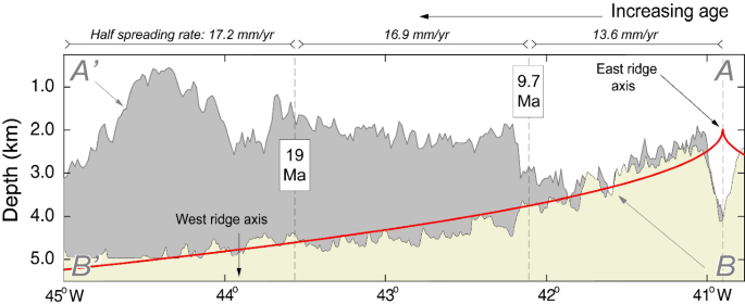

  

  Predicted thermal subsidence/age curve (thick red solid line), topographic profile (A–A′, location in Fig. 8a) along the Vema Transverse Ridge crest (dark gray shaded) and topography along a seafloor-spreading flow-line (B–B′, location in Fig. 8a) starting at mid-point of the eastern MAR segment (light yellow shaded profile). Ages are calculated from Euler vectors of Shaw and Cande [55] and geomagnetic timescale of Cande and Kent [202]. Ages at magnetic chrons 5 and 6 are indicated as black boxes

  Fig. 11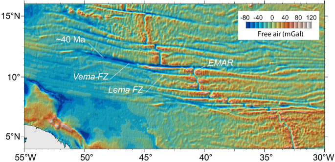

  

  Satellite-derived gravity image of the Central Atlantic [161], where the Vema fracture zone (FZ), the transverse ridge and the long-lived EMAR segment can be identified

• 2. The Vema transverse ridge rises abruptly in ~ 10-Ma-old crust ~ 140 km from the eastern Ridge-Transform intersection (RTI); it extends for ~ 300 km as a narrow asymmetric topographic feature parallel to the Vema Transform, reaching over 3 km above the crustal thermal contraction level; it then drops abruptly in ~ 26 Ma lithosphere (Fig. 10). The crest of the VTR tends to become shallower with distance from the RTI. Seismic reflection profiles revealed that the western shallowest ~ 50 km long portion of the VTR is capped by a carbonate platform up to 500 m thick (Fig. 12). The reflector at the base of the carbonate cap is nearly horizontal, suggesting that the top of the VTR reached above sea level; it was then eroded and capped by Pliocene to mid Miocene shallow-water carbonates during subsidence [50, 51].

  Fig. 12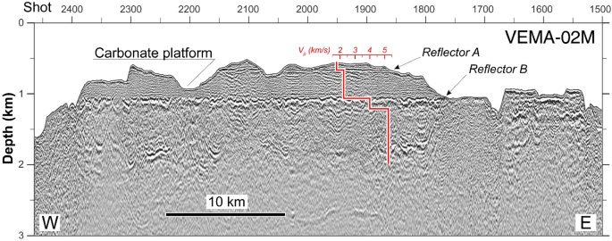

  

  Portion of the multichannel seismic profile VEMA-02 M running along the Vema Transverse Ridge crest (post-stack finite-difference depth migrated section). A P-wave velocity profile is shown in the middle of the section. Note a prominent horizontal reflector (reflector B), interpreted as the eroded top of the basaltic crust, overlain by a carbonate platform. Reflector A marks a major unconformity within the shallow-water carbonate sedimentary sequence. Profile location is indicated in Fig. 8b

The northern slope of the VTR exposes all the units of the oceanic lithosphere: one km thick mantle peridotite unit overlain by a several hundred meters thick gabbroic unit; by a well-formed dyke complex and by an upper layer of massive basalts (Fig. 13). We defined this as the “Vema Lithospheric Section” (VLS), that represents the edge of a lithospheric sliver created steadily by an 80 km long MAR axial segment (EMAR segment, Fig. 8a). A first study of the VLS detected a steady increase of crustal thickness and of mantle degree of melting from ~ 18 to 5 Ma [49]. Additional sampling of the VLS, carried out in 2005, extended the coverage of the mantle peridotites sampled along the VLS from crustal ages 26–2 Ma [52].

Fig. 13

N–S multichannel seismic reflection profile VEMA-06 M running perpendicular to the Vema transform and above the Nautile submersible sections (~ 42° 42′ W). a post-stack finite-difference time migrated section. b Interpreted line drawing. Lithology of the VLS is based on submersible observations and sampling. A reflector roughly parallel to the southern slope of the Vema transverse ridge (layer 2A), about 0.5 s (two-way travel time, TWT) below the sea floor, can be traced to the northern slope, where the boundary basalt/dyke complex was observed by submersible. The principal transform displacement zone (PTDZ) is marked by a furrow with recent deformation affecting the sedimentary sequence in a wide area on the southern side of the fault

In contrast to the VLS exposed along the northern scarp of the transverse ridge, the southern slope exposes mostly basalts, suggesting that the transverse ridge represents the edge of a flexured slab of oceanic lithosphere (Fig. 13).

An intensive program of rock sampling focused on the VLS shed light on 26 million years of evolution of its lithospheric composition and thermal state. Mantle ultramafics at the base of the VLS were sampled at over 40 sites (Fig. 10) covering crustal ages from 26 to 2 Ma [49, 52].

They can be separated in two different suites: an “older suite” from lithospheric age 26–18.5 Ma, and a “younger suite” from 16.5 to 2 Ma [52]. The older (26–18.5 Ma) mantle peridotites have a major element composition different from that of the younger (16–2 Ma) peridotites: the Ca/Al ratio of mantle-equilibrated cpx is for a given spinel Cr# higher in the younger than in the older group [52]. This suggest that the mantle source for the VLS sequence modified between 18 and 16.5 Ma not only its thermal structure but also its composition. The low cpx Ca/Al ratio of the older suite may be due to a higher proportion of melting in the garnet stability field, where cpx would melt ~ 10 times faster than garnet, depleting the residue of Ca [53]. Alternatively, the source of the younger suite might contain a higher garnet/cpx ratio, or a lower pyroxenitic component [54] than the source of the older suite.

VLS ultramafics show a trend of increasing degree of partial melting from ~ 16.5 to 2 Ma, together with an increase of crustal thickness inferred from the mantle Bouguer anomaly calculated from satellite gravity. Superimposed on this trend some 3–4 Myrs oscillations were observed (Fig. 14). This general trend is interrupted by a 1.4 Myrs long ultramafic mylonite interval from 18.2 to 16.8 Ma, possibly due to a relatively cold and/or highly depleted mantle source causing nearly amagmatic tectonic lithospheric accretion [52]. The oldest portion of this mantle sequence, from 26 to 18 Ma, shows a steady or slightly decreasing degree of melting up to the short mylonitic interval (Fig. 14); a possible explanation is the presence in the source of a low-solidus pyroxenitic component, that subtracts latent heat from the system during melting and cools the peridotitic mantle [54]. Thus, the mylonitic thermal minimum separates the older 26–18 Ma sequence from the younger 16.5–2 Ma sequence.

Fig. 14

Temporal variations of crustal accretion. a Residual Mantle Bouguer Anomaly (black solid line) and inferred variations of crustal thickness ΔH (dotted gray line) as measured along flow line B–B′ (location in Fig. 8a) starting from the mid-point of EMAR segment. Black dashed line refers to a linear regression fit of RMBA showing thickening of the crust moving towards the ridge axis, while half spreading rates, indicated at the bottom of the diagram, decrease toward younger ages. b Lateral variations of Cr# in spinel of mantle-derived peridotites (black hollow diamonds) and milonites (gray filled diamonds) sampled along the VLS [52]. c Temporal variations of single-cpx temperature of equilibration of peridotites estimated according to Nimis and Taylor [31]. The temporal variation curve of crustal thickness (a) is shifted by ~ 34 km (~ 2.2 Ma) with respect to the mantle degree of melting curve (b)

• 3. Spreading half rate of the lithosphere south of the transform, estimated from plate motion reconstructions of Shaw and Cande [55] (1988), varied from 13.6 mm/year between 0 and 10 Ma; to 16.9 mm/year between 10 and 19 Ma and to 17.2 mm/year between 19 and 26 Ma (Fig. 10). These estimated rates are in line with absolute ages obtained from zircon extracted from gabbros [56] and from ⁴⁰Ar/³⁹Ar ages of basalt (Cipriani pers. comm.), both exposed on the VLS (Fig. 10). We note that spreading rates decrease towards younger crustal ages, although mantle degrees of melting increase towards younger crustal ages.

• 4. The transform valley is floored about 5200 m below sea level by nearly horizontal sedimentary deposits up to 1 km thick (Fig. 8b); they are probably Pleistocene turbiditic sediments derived from the South America’s shelf [57], with also a local contribution from detrital and biogenous components derived from the walls of the transform valley [58]. The nearly horizontal sediment surface is interrupted by an E–W narrow disturbance running along the active part of the transform (Fig. 8a), interpreted as marking the trace of transform motion [59, 60], i.e., the principal displacement fault zone (PDFZ). Limited stretches of this transform trace are marked by linear narrow basaltic intrusions surfacing from the sediment cover (Fig. 8a).

2.2.2 Gravity-derived crustal thickness

Calculation of the mantle Bouguer anomaly from satellite and ship-board gravity data, corrected for lithospheric cooling with age, led to a residual mantle Bouguer anomaly (RMBA) versus time curve (Fig. 14a) and to an estimate of temporal variations of crustal thickness [52]. This crust, generated at the center of the EMAR segment, has a nearly constant average thickness from 26 to 20 Ma; it then increases steadily in thickness from ~ 20 Ma to present (Fig. 14a). Superimposed on this trend we observed 3–4 Myr oscillations of crustal thickness (Fig. 14a), interpreted as due to secondary convection in the subridge, H₂O-containing low-viscosity mantle that underlies a high viscosity, H₂O-poor residual mantle [49].

2.2.3 Upper mantle peridotite composition

100Cr/(Cr + Al) ratios of mantle-equilibrated spinel and orthopyroxene in VLS peridotites increase steadily from about 16.5 Ma (crustal age) towards ridge axis, indicating a steady increase through time of the degree of melting of the mantle upwelling below the EMAR axial segment. Oscillations in the degree of melting were detected, with wavelengths (3–4 Myr) similar to those observed in the RMBA profile, although offset spatially. Extending this curve to older ages thanks to the newly obtained samples shows that between ~ 26 and 19 Myr the mantle degree of melting underwent a weak tendency toward decreasing with time [52] (Fig. 14b).

Two pyroxene equilibration temperatures [30] reflect closure temperatures of chemical exchanges between pyroxenes within the peridotite system during ascent and cooling. Low velocity of ascent allows better equilibration under decreasing temperatures [32]. Thus, high equilibration temperature may reflect high upwelling velocity of the mantle, and vice versa. The calculated temperatures tend to decrease slightly from ~ 26 to 18.5 Ma along the VLS (Fig. 14c) but then increase from 16.5 to ~ 2 Ma, in parallel to the increase of mantle degree of melting.

2.2.4 Summary

The results summarized above suggest that temperature and/or fertility of the mantle that ascended below the EMAR segment at 10°–11° N decreased slightly from 26 to 18 Ma but then increased steadily from ~ 16.5 to 2 Ma. As noted by Bonatti et al. [49], the 16.5–2 Ma temporal increase of mantle temperature and/or fertility does not correlate with spreading velocity of that stripe of South American plate generated at the EMAR segment: spreading rate appears not to have increased, but rather to have decreased slightly along the VLS during the last 20 Myr (Fig. 10), as was discussed in Sect. 4 above.

The gradual increase of mantle temperature/fertility from ~ 16.5 to ~ 2 Ma at the 10°–11° N EMAR segment is paralleled by similar increases observed in zero-age MAR segments to the north, up to the Azores swell. Residual mantle Bouguer anomaly profiles oriented normal to ridge axis across segment midpoints between 28° and 31° 30′ N suggest an increase of crustal thickness from ~ 10 Ma to the present ridge axis; superimposed on this trend 2–3 Myr wavelength oscillations were detected [61,62,63]. Across-axis profiles between 20° and 24° N also hint at an increase of crustal thickness from ~ 8 Ma to present [64]. These data suggest that the increase of subridge mantle temperature and/or fertility may have been a general feature of the MAR between the Azores swell and the equator, although it was not accompanied by an increase in spreading rate.

Trends of temporal increase of mantle’s degree of melting from ~ 16.5 Ma to present at 11° N, combined with trends of zero-age decreasing degree of melting from Iceland to the equator (Fig. 5) lead to different possibilities. One is that the asthenospheric mantle presently upwelling below the Mid Atlantic Ridge becomes colder and/or less fertile moving from Iceland to the equator. We consider the possibility of “waves” of hot and fertile mantle flowing southward along the MAR from the Iceland and Azores plumes. We speculate that this south flowing zero-age hot/fertile mantle may be somehow connected with the temporal increase of hot/fertile mantle that we observed in the last 16 Ma at the 11° N. MAR segment.

Plate divergence and the formation of new lithosphere along oceanic spreading centers involves a variety of complex and interrelated processes: the asthenospheric mantle upwells beneath spreading centers; melt generated by partial melting of the upwelling mantle segregates from the deforming solid matrix and migrates toward the ridge axis; the extraction and solidification of melt creates the oceanic crust; and the cooling of the crust and upper mantle, away from ridge axis, forms the oceanic lithosphere. These processes are controlled mainly by the thermal state of the lithosphere beneath mid ocean ridges, which is influenced by the relative velocity between spreading plates, and by the occurrence of major ridge discontinuities, such as transform faults.

2.3 Northern Mid Atlantic Ridge: geology and evolution

Plate boundary geometry, seafloor spreading and melt productivity determine the geology and the tectonic setting of mid ocean ridge segments and transforms. Changes in plate kinematics can induce changes in plate boundary geometry that will tend toward a new equilibrium both by triggering new tectonics and by rejuvenating previous structures.

2.3.1 Geology of ridge segments

Two modes of lithospheric accretion (symmetric and asymmetric) characterize slow spreading ridges such as the MAR. The first mode generates a symmetric seafloor morphology on both side of the ridge axis, fitting the classic mid ocean ridge model. Seafloor spreading is accommodated along a ridge segment by the interplay between short-offset high-angle normal faults dipping toward ridge axis, and lava flows fed by dikes intruding the axial zone and forming a layered magmatic crust and linear, ridge-parallel abyssal hills (Fig. 15). Seismicity is prevalent at segment ends in the proximity of ridge–transform intersections (RTIs) where nodal basins form bounded by high-angle normal faults [65] (Fig. 15). In addition, a large topographic high occurs in RTIs at the active inner corner of the plate boundary, called “high inside corner”, while the “outside corner” across the spreading center, is often anomalously low [66].

Fig. 15

Topography of the Vema eastern ridge–transform intersection. Note the prominent median ridge that rises more than 1000 m above the transform valley seafloor. Geological observations from Nautile dives suggest an extensional origin for the median ridge [110]. Numbered white circles and red lines indicate locations of Nautile dives [47, 110]. White solid line marks location of the transform fault plane

At slow spreading ridges, where large long-lived faults may develop parallel to ridge axis, seawater penetrating deep along the fault zone chemically alters the rocks and weakens the fault. Continued extension and slipping along the weakened fault zone allows flexural rotation of a large block of seafloor forming an enormous domal mountain, named “oceanic core complex” (OCC) that can expose deep seated crust and mantle rocks [67,68,69,70,71]. In this model of lithosphere accretion, oceanic detachment faults initiate as high-angle normal faults at depth, and turn into shallow low angle extensional faults through rotation of the footwall. This type of seafloor spreading may represent a distinct mode of lithosphere accretion at slow mid ocean ridges that does not fit the classical “Penrose” model of oceanic crustal accretion [72]. Diking and volcanism at ridge axis are lower than in more normal, symmetrically seafloor spreading [73, 74], with melt intrusions in the footwall of the detachment fault forming gabbro bodies [75, 76]. Thus, seafloor spreading becomes asymmetrical, with large tectonic blocks exposing lower oceanic crust and mantle on one side of the ridge segment, and with reduced magmatic crust on the other side. OCCs commonly develop at the inside corner of ridge–transform intersections; examples include Charlie Gibbs (MAR 52.5° N) [25], Atlantis Massif (MAR 30° N, Fig. 16a) [67, 77,78,79,80], and the Kane OCC (MAR 23° N) [80]. However, core complexes have been identified in the mid zone of spreading segments (Fig. 16b), where adjacent OCCs may have resulted from movement along a single detachment fault [68, 69, 82, 83]. Large fields of OCCs have been also observed off-axis along the MAR, probably formed by the persistence for several million years of conditions suitable for the formation of detachment faults [68, 69, 83,84,85].

Fig. 16

Oceanic core complex. a 3D view of the Atlantis Massif bathymetry from southeast. The OCC develops at the inside corner of the eastern intersection between MAR and Atlantis Transform. b High-resolution 3D view from southeast of the 13° 20′ N OCC investigated by Escartin et al. [231] with AUV microbathymetry. High-resolution bathymetry reveals details of the main morphological features of an OCC, i.e., corrugated surface, breakaway and termination zones. This OCC has been identified in the mid zone of a spreading segment

Processes that control lithospheric accretion mode (symmetric or asymmetric) along slow ridges remain not fully understood, although they differ significantly even as far as the geochemistry of associated rocks [72]. Basalts from symmetrical segments show lower compositional variability and lower eruption temperatures than those from asymmetrical segments with more primitive compositions and lower crystal fractionation, higher Na₂O and FeO and lower CaO [72]. It is not yet clear why a fault should continue to extend and to roll over for several million years to form an OCC, while another stops after having extended for a relatively short time. Long-lived detachment faults with large-scale corrugations have been identified on magma-poor mid ocean ridges; however, recent studies and numerical models simulating lithospheric accretion at a ridge segment including melt productivity and lithosphere faulting suggest that detachment faults form when magma supply is relatively low, i.e., when ~ 30–50% of total extension is accommodated by magmatic accretion and when there is significant magmatic addition in the fault footwalls [71,72,73,74, 76, 82,83,84,85].

2.3.2 Transform-related tectonics

Transform faults consist commonly of a single narrow strike-slip zone (a few km wide) offsetting two mid ocean ridge segment and following a small circle path relative to the plate Euler pole location [40]. Oceanic transform faults, especially those with large-offset, are complex plate boundaries that can deform under the influence of far field stresses, especially changes in plate motion [44, 60, 86,87,88,89,90,91,92,93].

Not all transforms react equally to equivalent stress changes, suggesting the influence from offset length, spreading rates and mantle heterogeneities [15, 49, 94, 95]. The strike-slip movement is accommodated mainly along a shear zone a few hundred meters wide, called the “Principal Displacement Fault Zone” (PDFZ), where the stress may be partitioned locally, caused by a non-straight transform boundary due to bends of the fault trace and/or to restraining stepovers leading to local transpression or transtension, particularly at slow-slip long-offset transforms such as Vema, St Paul and Romanche. The Vema PDFZ is marked by a furrow, probably the trace of a sub-vertical fault affecting the entire sedimentary sequence (Fig. 17). Although the PTDZ appears to be very narrow at the sea floor (~ 0.5 km), we observe a wider and older deformation zone (~ 2.5 km) within the sediments south of the PTDZ. It consists of a gentle asymmetric fold draping a topographic high of the acoustic basement, suggesting a vertical or horizontal overstep related to local transpression (Fig. 17).

Fig. 17

Depth migrated close-up of the portion of the seismic reflection profile VEMA-06 M (Fig. 13) that crosses the transform valley

Transverse ridges are elongated reliefs parallel and adjacent to transform zones and their fracture zone extensions, i.e., normal to the axis of mid ocean ridges (Fig. 18). They are particularly well developed in slow-slip transforms, such as those offsetting the Mid Atlantic Ridge. Transverse ridges constitute major topographic anomalies relative to the “depth/square root of age” relationship [96]. They are a dominant factor in determining rough topography in wide regions of the ocean floor, such as the equatorial and northern central Atlantic.

Fig. 18

3D view of the Vema western ridge–transform intersection from northwest. Multibeam reflectivity, superimposed on the bathymetry, shows a high backscatter within the nodal basin, suggesting recent lava flows from the ridge axis that flood the nodal basin floor

A number of hypotheses have been put forward concerning the nature and origin of transverse ridges; most involve vertical movements of slivers of oceanic lithosphere, under the influence of buoyancy or tectonic forces: (a) thermal expansion and isostatic uplift of the old plate near the RTI induced by heat conduction from the young/hot side to the old/cold side of the transform [97, 98]; (b) thermal expansion and uplift of the lithosphere adjacent to the transform caused by shear heating due to friction along the active transform fault [99]; (c) uplift of the inside corner of the RTI due to frictional drag along the strike-slip fault that, decreasing with depth, triggers a twisting moment to the plate [99]; (d) extension across the transform fault induced by horizontal thermal contraction of the cooling plates causes upwelling of asthenospheric material into the resultant void flexing up both edges of the transform fault into transverse ridges [100]; (e) the old side of the fracture zone subsides slower than the young side, leading to flexure across the locked, aseismic part of the fracture zone [101]; (f) seawater penetrates deeply into the shattered lithosphere along the transform fault and hydrates upper mantle rocks, forming low-density serpentinite, which rises diapirically [86]; (g) upwelling of asthenospheric material along the spreading axis drags up the bounding walls of the conduit, including the wall formed by the edge of the old plate across the RTI [102, 103]; (h) the top of the lithosphere cools less than its bottom as the lithosphere ages causing a bending moment in the plate that flexures the unconstrained lateral edges of the transform fault [104]; (i) small changes in the direction of plate motion introduce an extensional or compressive component in the stress field along the transform that can cause vertical motions [64, 86, 95, 105, 106]; (j) strike-slip motion along a non-linear transform boundary causes either compression (with uplift) or extension (with pull-apart basins and subsidence) at bends in the boundary [86].

Multibeam data show that the MAR-parallel seafloor fabric south of the VTR shifts its orientation by 5°–10° clockwise in ~ 10–12 Myr-old crust (Fig. 8a), indicating a change at that time of the orientation of the MAR axis and of the position of the Euler rotation pole. Spreading half rate of the crust south of the transform decreased from 17.2 mm/year between 26 and ~ 19 Ma (chron c6n) to 16.9 mm/year between ~ 19 and 10 Ma (chron c5n), to 13.6 mm/year from ~ 10 Ma to present. Slowing down of spreading occurred close in time to the change in ridge/transform geometry, suggesting that the two events are related. This change caused extension normal to the transform, followed between 12 and 10 Ma ago by flexure of the edge of the lithospheric slab, uplift of the VTR at a rate of 2–4 mm/year, and exposure of the VLS at the northern edge of the slab, parallel to the Vema transform (Fig. 13). Ages of pelagic carbonates encrusting ultramafic rocks sampled at the base of the VLS at different distances from the MAR axis suggest that the entire VTR rose vertically as a single block within the active transform offset [107]. A 50 km long portion of the crest of the VTR rose above sea level, subsided, was truncated at sea level and covered by a carbonate platform [51, 64]. Subaerial and submarine erosion has removed material from the top of the VTR and has modified its slopes. A numerical model relates lithospheric flexure to extension normal to the transform, suggesting that the extent of uplift depends on the thickness of the brittle layer, consistent with the observed greater uplift of the older lithosphere along the VTR [44].

Median ridges are prominent topographic features located within transform valleys. They are found only in some RTIs along the MAR; in particular, at the RTIs of the Charlie Gibbs and Vema transforms [35, 108,109,110], of the Doldrums, St Paul and Romache transform systems [15, 18, 45] and of the Chain transform [111]. Little is known about the geology and deep structure of median ridges; however, recent studies have shown that they may be related to changes in plate boundary geometry leading to transpression or transtension within the transform domain. Median ridges due to transpression along the MAR consist of serpentinized and mylonitized upper mantle rocks, such as the Atoba ridge near the western RTI of the northern St Paul transform (Fig. 19a) [15, 112] and the median ridge near the Chain eastern RTI (Fig. 19b) [111]. Transtension related median ridges represent commonly slivers of uplifted oceanic lithosphere [110], such as the median ridge at the eastern RTI of Vema (Fig. 15), intensely investigated by Nautile dives [110, 113]. It is the main transform-parallel topographic feature of the Vema transform valley, rising up to ~ 1000 m above the adjacent seafloor and dividing the transform valley into a northern and southern valley (Fig. 15). It is an E–W elongated continuous ridge (~ 80 km long, 8 km wide) bounding to the North the present-day PDFZ from 41° 20′ W to the nodal basin (40° 52′ W) and ending at 40° 40′ W East of the RTI, outside the active fault zone. It reaches a minimum depth of 3755 m at 40° 58′ W. Immediately to the north of the tip of the EMAR axis, the crest of the median ridge is shallower and shows an arcuate shape (Fig. 15). Direct observations and samples recovered by Nautile dives from both flanks of the median ridge indicate that this uplifted sliver of oceanic lithosphere is covered by sedimentary deposits consisting of polymictic breccias, sandstones and siltstones composed of basaltic, doleritic, and gabbroic clasts, that underwent greenschist facies metamorphism prior to their disaggregation and sedimentation. [110]. The rapid emplacement of detrital gravitative deposits on the valley floor suggests that the median ridge emplacement is related to the major tectonic event that led to the the transverse ridge formation 12–10 Ma [44, 110].

Fig. 19

Compressive features within transform valleys. a Bathymetry of the St. Peter and St. Paul’s Massif, called Atoba ridge. Data are from Gasperini et al. [232]. Atoba Ridge forms a sigmoidal relief within the northern transform valley of the St Paul transform system culminating at St Peter and St Paul rocks [15, 51]. These islets are formed by variably serpentinized and mylonitized peridotites and are currently uplifting at rates of 1.5 mm/year [233]. The left overstep of the right-lateral St. Paul transform fault implies transpression in the St. Peter and St. Paul Rocks area. It has been recently suggested that the Atoba Ridge is caused by a long-lived transpression resulting from ridge overlap due to the propagation of the northern Mid Atlantic Ridge segment into the transform domain that induced migration and segmentation of the transform fault creating restraining stepovers [15]. b Bathymetry of the eastern sector of the Chain transform. Within the active transform fault zone, transpressive features with several en échelon fault scarps have been observed [111]

3 The subridge mantle below the Mid Atlantic Ridge

3.1 Mantle flow beneath mid ocean ridge segments

The velocity of mantle advection below ridge axis affects the subaxial temperature distribution, that in turn determines mantle melting and crust formation. Mantle flow and melting at spreading centers have been studied with fluid-mechanical calculations, including models where mantle flow is a response to the motion of overriding plates (passive flow), and models where the mantle flow is also driven by local buoyancy forces (dynamic flow).

3.1.1 Passive mantle flow

Passive flow models suggest mantle flow patterns shaped dominantly by viscous drag from rigid moving apart plates; they predict that melt is generated in a broad upwelling region (> 100 km across). Mantle flow velocities depend on spreading rate and on plate thickness geometry close to ridge axis. In models where plate thickness is constant, upwelling is less focused and the maximum vertical velocity is lower than the half spreading rate [114, 115]. In models where plate thickness increases rapidly with age upwelling is narrowly focused and its maximum vertical velocity can exceed the half spreading rate by up to ~ 30% [116, 117]. These models require mechanisms, such as viscous-stress-induced pressure gradients [118]; anisotropic permeability [119]; and local pressure gradients due to melt freezing near the bottom of the subsolidus lithosphere [120]. These mechanisms drive the melt laterally toward ridge axis. Melt concentration may be low (< 1–2%) throughout the entire melt production region if melt is efficiently extracted by porous flow. The upwelling flow pattern is mostly 2D except close to ridge–transform intersections where it becomes 3D.

3.1.2 Dynamic mantle flow and segmentation

Dynamic flow models may fit situations of low viscosity in the melting region, combined with buoyancy forces due to thermal and compositional density variations related to mantle depletion and melt retention [121,122,123]. These models require melt retention of at least several percent to provide buoyancy and reduce viscosity [124]. Mantle upwelling is then focused toward the spreading axis in a region as narrow as few kilometers; the upwelling velocity is much greater than the half spreading rate and melt transport is primarily vertical, driven simply by buoyancy. Numerical modeling of three-dimensional mantle upwelling along the MAR shows that buoyant mantle flow driven by temperature and compositional variations, including the effects of a small retained melt fraction (< 2%), generates instabilities that give rise to long-wavelength (> 150 km) segmentation [125,126,127]. Discontinuities and thermal perturbations inherited from the initial stages of spreading play a key role in focusing three-dimensional melt migration at the base of the lithosphere away from the discontinuities and toward segment centers. Thicker crust beneath the center of spreading segments requires either larger rates of melt production or the focusing toward segment centers of melt produced more uniformly along the axis. Three-dimensional melt migration modeling shows that even a moderate amount of along-axis melt focusing can produce the observed magmatic segmentation (30–100 km) [127, 128].

Diapiric upwelling from a layer of melt distributed uniformly at depth along the axis has been also suggested as a possible focusing mechanism [129, 130]. Our gravity inversion results from the Vema transform show that the inferred across-axis crustal thickness variations have wavelengths (40–60 km) similar to those observed along-axis at the MAR [19, 131,132,133] and they are strictly related to variations in melt production at ridge axis. In addition, the pattern of degree of melting increasing slowly in time followed by a rapid fall, as shown by numerical results for low mantle viscosity of Sotin and Parmentier [123], both suggest a dynamic mantle flow origin for short wavelength magmatic segmentation rather than an origin due purely to melt migration. On the other hand, our estimated vertical velocity of the upwelling mantle (as discussed below), similar to the half spreading rate, suggests that most of mantle flow is driven by plate motion. Therefore, we have the paradox that the observed temporal variations of crustal production are related to dynamic mantle flow, and the estimated mantle upwelling velocity to passive flow.

3.1.3 Velocity of mantle upwelling

The exposure of the Vema transverse ridge (Fig. 8a) has allowed us to dredge up and analyze rocks that would normally be deeply buried [49, 52]. These peridotites formed at the ridge–transform intersection and are all from the top of the melting column; therefore, they represent the highest extent of melting of the column that lies below each of them. At slow spreading segments, melt production beneath RTIs can be reduced [134, 135] and melt pooling in segment centered magma chambers may be laterally transported in dykes to segment ends [136, 137]. However, this should not affect the offset between the peridotite melting curve and the crustal thickness curve. We have therefore been able to measure an apparent time delay between changes in crustal thickness, as estimated from gravity, and changes in residual peridotite chemistry (i.e., degree of melting) over a ~ 26-million-year timescale. Our chain of logic derives from the following observations. The signals indicating crustal thickness and the extent of peridotite depletion show oscillations with a wavelength of about 60 km (corresponding to a 3–4-million-year frequency), superposed on an overall > 16-million-year trend of increasing peridotite depletion and crustal thickness (Fig. 14). The variations seen in the two signals are correlated, but there is a phase lag of 34 km (or some 2.2 million years of spreading time) between the signals. What is the meaning of the 34 km offset between the signals denoting residual peridotite degree of melting and crustal thickness? Melt migration is much faster than solid flow through the melting region, so there must be a time delay between melt extraction from a given parcel of peridotite to create basalts, and the eventual emplacement of that same residual peridotite at the base of the lithosphere. In other words, the oscillation signals carried by the melt volume and by peridotite chemistry propagate upwards at different speeds and are recorded at different times, being spatially offset by the plate spreading rate (Fig. 20). Thus, the phase lag between extent-of-melting signals from peridotite and from crustal thickness (assuming that the bulk of the melt separates at a depth of 35 km and that melt velocity can be taken as infinite) can be used to calculate a solid upwelling rate of 16.1 mm/year [52]. This is similar to the rate at which the plate is moving away from the ridge (14–17 mm/year), hence it is consistent with upwelling rates predicted by passive flow models.

Fig. 20

Cartoon showing how basalt (generated by partial melting of mantle peridotite during ascent below the ridge) becomes separated horizontally from its parent peridotite. If we can estimate the depth where melting occurs, the horizontal distance between basalt and its parent peridotite, translated as time, allows us to calculate the velocity of the rising solid mantle. a Melt is generated within the melting region in the subridge mantle. b Melt migrates upward faster than the mantle. c Melt is extracted and accretes crust at ridge axis. d Formed crust has moved away from ridge axis when the parent residual mantle rises toward the surface to be included in the upper oceanic lithosphere

Water in the upper mantle can play an important role in governing melt generation and melt transport paths beneath spreading centers [138, 139]. The amount of water present in the oceanic upper mantle [140, 141] is sufficient to deepen the peridotite solidus and allow partial melting in a region wider and deeper than what is expected for an anhydrous mantle [142] (Fig. 3). Geochemical analyses constraint depth of initial melting and melt productivity along an adiabatic ascending path. Trace element ratios, as Hf/Lu and U/Th, indicate that melting begins in the garnet–peridotite stability field, while MORB major element composition shows that melting occurs where spinel is a stable phase. These observations are compatible with a fractional melting model where melting initiates at a "water influenced" solidus. Melt productivity during hydrous melting (garnet–peridotite region) is scarce, due to the mantle low water content. A small melt fraction (1-2%) is produced before complete exhaustion of water, after which melting proceeds above a “dry solidus” (spinel–peridotite region) with a higher production rate [138, 142]. Experimental studies on olivine single crystals and on olivine aggregates [141,142,143,144,145] have shown that water reduces the creep strength of mantle rocks. Reduction of upper mantle viscosity, due to water in olivine, is at least two orders of magnitude lower than in dry conditions [138]. The solubility of water in olivine is much lower than in basalts; therefore, partial melting can increase the solid-matrix viscosity depleting water from olivine [144]. Numerical models, including the effects of non-uniform upper mantle rheology and of pressure-dependent melt production rate, permit 3D upwelling as a possible mechanism for magmatic segmentation at slow spreading ridges [146]. These numerical models, that include thermal and compositional buoyancy, predict melting and consequently crustal thickness oscillations with frequency and amplitude depending on mantle viscosity [123, 146].

The short-term oscillations of melt production (3–4 Myr) observed at the Vema transform can be explained if we assume a subridge rheological mantle stratification due to extraction of H₂O from the upwelling mantle in the deeper part (> 60 km) of the melting interval, resulting in a higher viscosity layer (~ 10²⁰ Pa s) overlying a low-viscosity zone (~ 10¹⁸ Pa s) (Fig. 21). Following water loss, the solid flow of the high-viscosity residue that undergoes “dry” melting within the upper layer, is mostly driven by plate separation (passive flow), because high viscosity precludes dynamic mantle flow [123]. The low-viscosity mantle within the “wet” melting region upwells following a compositional and thermal buoyant flow [123, 146]. As the mantle moves away from ridge axis, it becomes denser due to cooling and to its decreasing melt content, because of the melt’s upward migration, thus overcoming compositional buoyancy. According to numerical models, a dense plume forms and sinks periodically into the deeper mantle, giving rise to intermittent convective rolls, periodic enhanced upwelling and increased temperature at the top of the low-viscosity layer (Fig. 21). This increases melting below a ridge axis.

Fig. 21

Model of mantle upwelling and crustal accretion consistent with the observed variations of extent of melting and crustal thickness at the MAR eastern segment of Vema (EMAR). Crustal accretion results from mantle upwelling induced by non-uniform subridge mantle rheology, with a low-viscosity layer between two layers with higher viscosities. Blue and red arrows show direction of mantle flow. The viscosity profile (right panel) describes the effects of dehydration, of melt in the matrix, and of change in creep mechanism. High viscosity precludes compositional and thermal buoyant flow in the dry melting region, where solid flow is mostly driven by plate separation (corner flow). The low-viscosity layer favors intermittent plume-like enhanced upwelling and melting

3.2 N–S propagation of subridge hot mantle waves

The combination of (a) decrease from N to S of temperature and/or fertility of the mantle that upwells below the MAR, and (b) increase from ~ 16 Ma to today of the same parameters along the MAR south of the Azores swell, leads to a number of alternative hypotheses. One is that a hot (asthenospheric) mantle wave has been flowing southward below the MAR from the Azores plume since over 20 Ma. Another is that both plume and mid-ocean ridge activity have been fluctuating in intensity with long (over 10 Myr) temporal wavelength. A third possibility is that the MAR has migrated in the central Atlantic over mantle regions with different thermal properties and/or composition. Let us consider if any of these hypotheses is consistent with available data.

3.2.1 Subridge asthenospheric flow

Various models have been attempted to explain the longitudinal flow of asthenospheric material below ridge axis [147, 148]. According to Yale and Morgan [149] a low-viscosity asthenospheric channel located between a high viscosity asthenospheric lid above and a high-viscosity “mesosphere” below, can be fed by hot “plume” material at various locations both on and off mid-ocean ridges.

The injection of hot “plume” material into the asthenosphere creates pressure gradients that may induce “dynamic” asthenospheric flow. Plate-driven shear flow should be added to pressure-driven flow in a plate spreading direction. The velocity profile v_x within asthenosphere flowing along ridge is given by:

$$ v_{x} = \left( {\frac{{\nabla P(z^{2} - hz)}}{2\mu }} \right), $$

(1)

where $\nabla P$ is the pressure gradient, z is the distance from the base of the asthenosphere, h is the thickness of the asthenospheric channel and $\mu$ is the viscosity of the asthenosphere. Integrating the velocity profile over the thickness of the asthenosphere gives the asthenospheric flux q_x [149]:

$$ q_{x} = \int_{0}^{h} {v_{x} {\text{d}}z = \frac{{ - h^{3} \nabla P}}{12\mu }} . $$

(2)

Note that the flow of hot mantle material below the ridge depends strongly on the distribution of viscosity with depth. The extent to which transforms offsetting the ridge axis can hinder subridge mantle flow has been studied particularly along the Southwest Indian Ridge (SWIR) where large transform systems affect the flow of material from the Marion and Bouvet plumes [150, 151]. A transform offset has two main effects on the flow of shallow mantle along the ridge [151]: one, deflection of the flow; two, reduction of the flow, or even its complete stop. These effects are strongly dependent on the length of the transform offset and on slip rate along the transform, both of which influence subridge thermal structure and viscosity as the transform is approached. The flux reduction occurs not only downstream from the transform, but also upstream, because the cooling effect of the transform offset reduces the subridge low-viscosity channel as the transform is approached.

3.2.2 Mantle flow below the Mid Atlantic Ridge

The Iceland and the Azores plumes, i.e., the two major thermal/compositional mantle anomalies of the North Atlantic, may be the source of unusually hot/fertile asthenospheric mantle flowing along the Mid Atlantic Ridge. Vogt [33] first proposed hot plume mantle flowing southwards from Iceland below the Reykjanes Ridge, a suggestion supported by elemental and isotopic geochemical gradients in the Reykjanes basaltic crust [34, 152]. Based on the angle of south-pointing V-shaped topographic/structural patterns (Figs. 2, 7) and on spreading rate, a velocity of 100–200 mm/year has been estimated by Vogt [33] for the southward flow of the subridge mantle along the Reykjanes Ridge: this is one order of magnitude higher than spreading rate. This model has been refined and elaborated upon by more recent studies [153,154,155]. The ~ 300 km Charlie Gibbs transform offset at 52° N may constitute a major barrier to the southward flow of Iceland plume material, and to the northward flow of Azores plume material.

The Azores mantle plume differs significantly from the Iceland plume. It is characterized by: (a) high degree of melting of the subridge upwelling mantle as estimated both from the mineral chemistry of peridotites [36] and from the Na₈ content of basalts [38]; (b) low mantle equilibration temperatures determined by 2 px geothermometry of peridotites [36]; (c) low quenching temperature of erupting basalt, estimated with an olivine-glass thermometer [156]; (d) low ³He/⁴He ratio of MORB glasses [157]; (e) high concentrations of CO₂, H₂O and halogens in MORB glasses [158, 159]; (f) high ⁸⁷Sr/⁸⁶Sr of MORB glasses [160]. These data suggest that the Azores plume, in contrast to the Iceland plume, does not have a deep mantle origin, and may represent a melting anomaly due to fertile, “wet” mantle sources of relatively shallow origin. Its source might contain enriched, ancient continental mantle blobs recycled through the upper mantle [36, 158]. Regardless of its ultimate origin, the Azores plume constitutes a melting anomaly linked to a hotter and/or more fertile than normal mantle that has the capacity of being entrained and of flowing along the Mid Atlantic Ridge.

A number of observations point to the possibility of a hot mantle flux from the Azores swell southward along the Mid Atlantic Ridge. Satellite gravity imagery of the North-Central Atlantic [161] displays a V-shape pattern centered on the Mid Atlantic Ridge axis and pointing southward, suggesting south propagation of mantle thermal and/or compositional anomalies that cause swelling of the crust. The V-angle south of the Azores swell is roughly 18° (Fig. 22). If we assume an average spreading rate of 20 mm/year for the ridge at ~ 40° N since 10 Ma, the average velocity of propagation of the anomaly is ~ 60–65 mm/year.

Fig. 22

The Azores swell. a Satellite-derived gravity image of the Azores region [161]. b Magnetic anomalies. Data are from the EMAG2 Earth Magnetic Anomaly grid (2 arc-minute resolution) [234]. V-shaped features indicate propagating ridges along the Mid Atlantic Ridge axis south of the Azores due to ridge–hot spot interactions producing temporal and spatial variations in melt supply to the ridge axis. Yellow arrow indicates spreading direction. White solid lines mark location of pseudofaults

Thibaud et al. [133] found evidence of N–S propagation along the MAR from 40° N to 26° N, supporting mantle flow south from the Azores swell, that transform offsets such as Pico, Oceanographer, Hayes and Atlantis, were unable to prevent. A pulse of along-axis southward flow of Azores plume mantle was proposed by Vogt [162] and Cannat et al. [163] to have traveled at 60 mm/year in Miocene time, causing excess volcanism and anomalously thick crust. If the Azores plume material first reached the surface about 36 Ma [164] and assuming that it traveled south at ~ 100 mm/year, it would have reached 10°–11° N, i.e., the latitude of the exposed VLS, roughly between 6 and 8 Ma. However, 10°–11° N is where we documented an increase of temperature and/or fertility of the subridge mantle starting ~ 16 Ma [49, 52]. It appears unlikely, therefore, that the mantle increasing temperature and/or fertility at 10°–11° N was caused exclusively by Azores plume-derived flow. However, the MAR has probably interacted with plume-like mantle thermal/compositional anomalies in the central north Atlantic for ~ 85 Myr [164]. The Great Meteor seamount system on the African plate and conjugate structures on the North American plate as well as the New England seamount chain suggest plume-like activity in the region preceding the Azores plume.

3.2.3 Westward migration of the Mid Atlantic Ridge

Present‐day absolute plate motion models suggest that most mid‐ocean ridges are migrating relative to the stable deep mantle, with a plate moving faster than the other diverging plate [165,166,167,168,169]. These models predict that the slow spreading MAR system is migrating westward relative to the deep mantle. As a consequence, mantle upwells asymmetrically beneath spreading segments with higher upwelling rates beneath the plate that moves faster (North and South America) compared to the slower moving plate (Europe and Nubia) [170, 171]. This causes a contrasting melt supply at the tips of ridge segments offset by transform faults, and consequently, different axial morphologies on opposing RTIs [172,173,174]. Another possible consequence of ridge migration is that the MAR system has moved above mantle regions with different thermal regime and/or composition.

The observed long-term temporal variations of the degree of mantle melting estimated from spinel Cr# of the peridotites along the VLS [49, 52] anti-correlate with the degree of melting derived from basalt Na₈, although they converge to a common value in the youngest stretch of the VLS [54]. In agreement with thin crust inferred by the gravity inversion (Fig. 14), the older mantle peridotites record a relatively low extent of melting; in contrast, the genetically associated and isotopically enriched basalts display the lowest Na₈ values of the entire VLS, suggesting that they were generated by a higher degree of melting of their mantle source. An explanation of these contrasting proxies for mantle partial melting at mid ocean ridges may be a subridge variably veined mantle that hosts fertile and chemically enriched pyroxenites [54]. In fact, melting of low-T-melting components present in a mantle source subtracts heat from the surrounding matrix by incorporating it as latent heat of melting, lowering the extent of melt of the host peridotite [175,176,177,178,179]. The pyroxenites melt first, generating isotopically enriched melts with Na₈, and cooling the host mantle, thus lowering the degree of fusion of the peridotitic matrix in proportion to its pyroxenite content, similarly to what happens by varying the mantle potential temperature [54].

We conclude that the creation of new oceanic lithosphere along the Mid Atlantic Ridge may involve different mantle mechanisms: (1) a steady mantle convection; (2) a more episodic activity of mantle plumes; and (3) a ridge system migrating over mantle regions with different composition or thermal properties.

3.3 Temporal cycles of mid-ocean ridge activity

Over 40 years ago Vogt [162, 180] remarked that world-wide plume magmatism appears to have gone through alternating periods of enhanced and waning activity: for instance, the Hawaii, Iceland, Canary and Azores plumes were all highly active in the Tertiary roughly between 20 and 10 my ago and then again during the last couple million years. The Afar plume also peaked in the 20–10 my interval [181]. Vogt [162] argued that “if …. hot spots recorded global episodes (of enhanced activity), why not also the mid ocean ridges?”. We find Vogt’s question pertinent to our problem: mantle plume activity may not be independent of plate tectonics and may influence upper mantle thermal structure and convection [182], triggering enhanced mid ocean ridge activity even in areas far from plumes, where the ridge may not be directly affected by plume-derived material. For instance, an interval of increased mid ocean ridge activity occurred in upper Cretaceous times (~ 110–85 Ma) when a pulse of rapid spreading has been documented at most mid ocean ridges, particularly at the East Pacific Rise and in the central and southern Mid Atlantic Ridge [183,184,185].

4 Conclusions

The data reviewed in this paper confirm that the Earth’s oceans are carpeted by a solid, relatively rigid but mobile lithosphere, underlain by hot less viscous convecting mantle asthenosphere. This scheme reflects essentially concepts injected in our culture half a century ago with the theory of “Plate Tectonics”. The large majority of Earth scientists up to about 1960 believed in a relatively fixed and stable position of the continents on the Globe, and in very ancient, relatively “quiet” ocean basins. However, about 10 years later the large majority of the scientific community had changed their mind, and believed in continents modifying continuously their position on the Globe (i.e., continental drift) and ocean basins being relatively young, “hot” and active features of the Earth. The amazing rapidity of this major paradigm shift in our view of the Earth gives support to the ideas of Kuhn [186], who suggested that progress in the sciences occurs by means of short “scientific revolutions”, with long periods of relative stability in between. The “Plate Tectonics” revolution of 50 years ago was followed by a period of relative stability, during which the theory has been refined, also thanks to new data and interpretations, as illustrated in this paper.

However, let us not relax, let us keep alert, because the next revolution may arrive while we least expect it!

Appendices

Appendix 1: The Vema transform: data and methods

The Vema FZ data discussed in this paper were obtained by a number of research vessels, starting with the R/V Vema that in early sixties first identified this feature [39]. Concerning more recent work involving the authors of the present paper, we can mention the following:

• (a) Cruise S45 carried out in 2019 with R/V N. A. Strakhov of the Russian Academy of Science. Multibeam bathymetry, magnetics and seafloor sampling [45];

• (b) Cruise S22 carried out in 2000 with R/V N. A. Strakhov. Multibeam bathymetry, magnetics and seafloor sampling [49].

• (c) Cruise S19, in 1998 with R/V N. A. Strakhov. Multibeam bathymetry, multichannel reflection seismic and magnetics, seafloor sampling [43].

• (d) Cruise EW9305, in 1993 with R/V M. Ewing of Columbia University’s Lamont Doherty Earth Observatory. Multibeam bathymetry, gravity and magnetics, seafloor photographs and sampling [187].

• (e) Cruise VEMA92, in 1992 with R/V OGS Explora of Istituto Nazionale di Oceanografia e Geofisica Sperimentale. Multichannel seismic reflection survey and magnetics [188].

• (f) Cruise VEMANAUTE carried out in 1988 with French submarine Nautile, observation and sampling of VLS, and eastern median ridge and RTI [47, 110, 113].

• (g) Deep Sea Drilling Project (DSDP) Leg 4 of the R/V Glomar Challenger (1969), drilling site 26A [57].

1.1 Bathymetry

Multibeam coverage of much of the investigated area was achieved during our cruises using different multibeam systems: (1) during cruise S45 we used a RESON SEABAT 7150 system [45], that operated at a frequency of 12 kHz and consisted of 256 beams across a 150° swath width (i.e., ~ 7 times the water depth); (2) during cruise S22 we used a KONSBERG EM12S system, that operated at a frequency of 13 kHz and consisted of 81 beams covering a swath width of 2 times the water depth; (3) during cruise S19, we used a HOLLMING ECHOS 625 system [43], consisting of 15 (12.5 kHz) beams covering a swath of seafloor roughly 2/3 of the water depth; (4) during LDEO cruise EW9305 [187] we used a Hydrosweep HS-DS (Atlas-Krupp) system operating at 12 kHz and consisting of 59 beams across a 90° swath width (2 times the water depth). Multibeam data were merged with raw data extracted from the NGDC Bathymetry Database (cruises: KN162L07, KN162L08 and KN192-04, R/V Knorr, 2002 and 2007) and with those from cruise SO181 (R/V Sonne, 2018) [46]. They were filtered and processed at ISMAR-CNR by the Kongsberg Neptune/Poseidon packages; spatial analysis and mapping were performed using the PLOTMAP [189] software. Digital terrain models and reflectivity images were produced down to a horizontal resolution of 60 m (Figs. 8a, 18).

1.2 Gravity

Gravity data were collected with a Bodenseewerks KSS-30 sea gravimeter during cruise EW9305, navigated by Global Positioning System [187]. Gravity values were recorded at 6-s intervals and smoothed with mean value every 60 s corresponding to an average distance of 250 m between data points registered during geophysical profiling (speed 7–8 knots).

Fig. 23

Cross-over errors of gravity data from the Vema transform region. a Histogram showing cross-over differences of marine gravity profiles collected during the EW-9305 expedition before leveling and adjustments. b Frequency distribution of cross-over errors among gravity profiles of all cruises before and c after leveling and adjustments

Gravity reference points were obtained at the beginning and the end of the expedition. The normal field, Eotvos correction and an estimated time dependent field (related to drift of the gravimeter) have been separated from the gravity data to obtain residuals. The normal gravity field has been calculated using the 1980 Geodetic Reference System [190] according to:

$$ \gamma_{0} = \gamma_{e} \left[ {1 + k_{1} \sin^{2} (\phi ) - k_{2} \sin^{2} (2\phi )} \right] $$

(3)

with coefficients k₁ = 0.005302357, k₂ = 5.869 10^–6 and γ_e = 978,032.7 mGal, γ₀ the normal gravity and ϕ the geographical latitude. The internal consistency based on statistics at 172 cross-over points gives an accuracy estimate of 1.15 mGal (Fig. 23a). These data have been complemented by those of Prince and Forsyth [41] and by those extracted from the NGDC database (Fig. 24a), to produce the free air gravity map. A total of 31,872 gravity measurements was used. The overall statistics at 755 cross-over points give a mean and standard deviation of 4.7 and 11.6 mGal, respectively (Fig. 23b). These data were collected over a 20-year period, during which recording instruments and navigation systems greatly improved. To integrate these different data sets before merging, the ship gravity for each line was adjusted in a least-square sense by applying a series of corrections aimed at reducing the errors at cross-over points and at matching the satellite-derived marine gravity field (Appendix 2).

Fig. 24

Combining shipborne and satellite gravity data. a Interpolated bathymetry and gravity lines in the study area. Solid red lines indicate EW9305 coverage; black lines indicate data from Prince and Forsyth [41]. b Free air satellite-derived gravity anomalies [161]. c Combined ship-borne and satellite-derived gravity field. d Residuals between (c) and (b)

Altimetric satellite data, collected since the eighties, have been used to produce geoid height and free air gravity anomalies over all the ocean basins, allowing a global coverage up to high latitudes with high accuracy and resolution. Comparing altimetric-derived and ship gravity data has shown that significant information is absent in the 20–40 km wavelength range of the satellite-derived gravity field, limiting the usefulness of the satellite data to determine local variations in crustal thickness [191,192,193]. Blending multi-satellite and ship-borne gravity data allows merging of short wavelength components in the marine gravity field. Thus, when ship gravity data are available in addition to altimetric data, these heterogeneous data have to be combined in an optimal way, to determine the gravity field with the best possible coverage and resolution. Figure 25a shows a comparison between ship and satellite-derived gravity anomalies interpolated onto the same ship track from the gravity field computed by Sandwell et al. [161] on a 1′ × 1′ grid (release 30). The observed minimum DC offset is − 1.9 mGal (cruise K020A), while the maximum is 19.1 mGal (cruise EW9305). The large DC component of the EW9305 data reflects the error due to the tie point correction, probably referred to Postdam 1930 Datum. The largest differences were recorded along the shallowest portion of the Vema transverse ridge where the difference at the crest reaches about 80 mGal, probably due to lack of short wavelength components in the satellite-derived gravity.

Fig. 25

Comparison of ship-borne and satellite gravity data. a Black solid line indicates ship-borne free air anomaly, while the red dashed line indicates the satellite-derived gravity data along the same ship track. b Spectral coherence between satellite-derived and ship-board free air anomalies

The resolution of the satellite data has been estimated thorough the spectral coherence between the satellite and the ship-board gravity profiles, defined as

$$ \gamma_{{\Delta g_{a} \Delta g_{s} }}^{2} (k) = \frac{{\left| {P_{{\Delta g_{a} \Delta g_{s} }} \left( k \right)} \right|^{2} }}{{P_{{\Delta g_{s} \Delta g_{s} }} \left( k \right)P_{{\Delta g_{a} \Delta g_{a} }} \left( k \right)}}, $$

(4)

where $P_{{\Delta g_{s} \Delta g_{s} }}$ and $P_{{\Delta g_{a} \Delta g_{a} }}$ are the power spectral densities and $P_{{\Delta g_{s} \Delta g_{a} }}$ is the cross-spectral density of data series. Spectral coherence estimates measure the degree to which ship-borne and satellite gravity data are linearly related at a given wave-number. Because ship-board profiles are relatively short and dominated by long-wavelength anomalies, power spectral densities have been estimated on a single line for each survey obtained by tapering and linking the individual profiles. The spectral estimates were obtained using the discrete Fourier transform of the auto and cross-correlation functions, as discussed in Jenkins and Watts [194]. The spectrum is smoothed using Parzen window to reduce the variance of the spectral estimates. The coherence estimates, with 95% confidence, are shown in Fig. 25b. The confidence intervals for coherences < 0.5 are not plotted. The coherence between satellite and ship-board gravity stays close to one at wavelengths greater than 80 km, but it falls off sharply at higher frequencies, falling down to 0.5 at wavelengths of 22–24 km and close to zero at wavelength shorter than 15 km.

Systematic errors account for some of the differences between satellite and ship-board gravity; in fact, as shown in Fig. 25a, ship gravity is offset from satellite gravity and the offset varies with time. We reduced these differences adjusting the ship gravity data in order to predict a combined gravity field. The deviation δ_g between the ship gravity and satellite gravity anomalies, at wavelengths greater than a given λ_c, can be related to the use of different reference ellipsoids and to the long-wavelength errors affecting ship data, such as non-linear mechanical drift of gravimeter, incorrect ties to base stations and off-leveling [195]. It has been shown that a combined model of general and trigonometric polynomials is more advantageous to describe the change of systematic error [196]. We assume that the deviation δ_g can be characterized by a constant correction for each surveying line [41] and by a time function for successive lines of a survey [197] as:

$$ \delta_{g}^{i} (t) = x_{0}^{i} + \sum\limits_{k = 1}^{N} {x_{k}^{j} t^{k} + } \sum\limits_{k = 1}^{M} {\left[ {x_{2k + N - 1}^{j} \cos \left( {k\omega^{j} t} \right) + x_{2k + N}^{j} \sin \left( {k\omega^{j} t} \right)} \right]} , $$

(5)

where N and M are positive integers; t is time from the beginning of the jth survey; $\omega = 2\pi /(t_{{\text{e}}} - t_{{\text{b}}} )$ is the angular frequency; $t_{{\text{e}}}^{j}$ and $t_{{\text{b}}}^{j}$ are the end and beginning times of the survey; $x_{0}^{i}$ and $x_{k}^{i}$ are the unknown model parameters for the ith line of the jth survey. The unknown parameters of the error model describing changes of systematic error that affects ship gravity data (Eq. 5), were evaluated based on a least-squares estimate (see Appendix 2). The compensation of systematic errors outlined above has a twofold effect: it reduces the cross-over differences and it adjusts ship gravity to the satellite-derived gravity field. After adjustment, the mean and rms differences between ship and satellite gravity are 0.4 and 7.1 mGal, and the overall cross-track discrepancies are reduced to zero mean and standard deviation of 3.7 mGal, equivalent to an accuracy of 2.6 mGal (Fig. 23c). The adjusted ship gravity is then included with satellite-derived gravity to derive a second gravity field (Fig. 24). Different techniques were developed during the last few years to combine ship-borne and satellite-derived gravity data, such as least-squares collocation [195], least-squares adjustment in the frequency domain [198], and input–output system theory [199, 200]. Studies on simulated [200] and real data [201] have shown that the best results are obtained by the input–output system theory (IOST) method, mainly when the power spectral densities are estimated directly from the data. The use of IOST requires the field of observables be given on the same grid with known error power spectral densities. Ship gravity anomalies were computed on the same grid of Sandwell et al. [161] (release 30) satellite-derived global gravity for the area of interest. We assume gravity anomalies affected by a Gaussian random noise with zero mean and variance of 6.76 mGal² and 25 mGal² for ship-board and satellite-derived gravity data, respectively. The IOST estimated values for the free air anomalies are given by:

$$ F\left\{ {\Delta \hat{g}} \right\} = F\left\{ {\Delta g_{s} } \right\}\left[ {1 + \frac{{E_{{\Delta g_{s} \Delta g_{s} }} }}{{P_{{\Delta g_{s} \Delta g_{s} }} }}\frac{{\left( {P_{{\Delta g_{a} \Delta g_{a} }} + E_{{\Delta g_{a} \Delta g_{a} }} } \right)}}{{E_{{\Delta g_{a} \Delta g_{a} }} }}} \right]^{ - 1} + F\left\{ {\Delta g_{a} } \right\}\left[ {1 + \frac{{E_{{\Delta g_{a} \Delta g_{a} }} }}{{P_{{\Delta g_{a} \Delta g_{a} }} }}\frac{{\left( {P_{{\Delta g_{s} \Delta g_{s} }} + E_{{\Delta g_{s} \Delta g_{s} }} } \right)}}{{E_{{\Delta g_{s} \Delta g_{s} }} }}} \right]^{ - 1} , $$

(6)

where F is the 2D Fourier transform operator, $P_{{\Delta g_{s} \Delta g_{s} }}$, $P_{{\Delta g_{a} \Delta g_{a} }}$, $E_{{\Delta g_{s} \Delta g_{s} }}$ and $E_{{\Delta g_{a} \Delta g_{a} }}$ are the power spectral densities of ship-board and satellite-derived gravity data and noise, respectively. Figure 24 shows the result of the procedure we have applied; although the signature of the satellite only (Fig. 24b) and the combined gravity field (Fig. 24d) appear to be quite similar overall, much of the detailed structures along the Vema transverse ridge have come from the ship data (Fig. 24c).

1.3 Magnetics

The Vema Fracture Zone is located close to the magnetic equator where the geomagnetic field is horizontal causing magnetic anomalies to be very weak (some tens or a few hundred nT) relative to the ambient noise. Furthermore, diurnal variations of the magnetic field may reach peaks of hundreds of nT due to the effect of the equatorial electroject, an electric current which travels around the E region of the Earth's ionosphere. In addition, in the vicinity of a transform offset, where differently magnetized blocks may face each other, further complexity is introduced, because location, strike, and polarity of crustal magnetic anomalies are distorted relative to their source bodies. However, careful processing of the magnetic data can help obtain useful information to deduce the tectonic evolution of the area.

We merged all the magnetic lines available from the Marine Trackline Geophysical Data (NOAA, 1977) with those acquired during R/V Strakhov S19 and S22 cruises in 1998 and 2000 [43, 49] where a magnetometer, based on the Overhauser effect, was deployed at a distance of 230 m from the GPS antenna. Most of the magnetic lines are oriented E–W, parallel to seafloor spreading, others are aligned N–S, crossing the fracture zone perpendicularly, while the oblique lines are few. We combined a total of 88,567 measurements of the total magnetic field acquired over a time span of 33 years (1967–2000) and over an area extending from 10° to 12° N and 45° to 38° W. The magnitude of the magnetic field varies from 30,700 nT to 34,800 nT (Fig. 26).

Fig. 26

Compilation of magnetic data in the Vema transform region collected during the geophysical surveys carried out in the area from 1967 to 2000. a Total field (raw data). Magnetic profiles are superimposed (gray lines). b Magnetic anomalies after IGRF removal, diurnal variations correction, filtering and leveling. c Analytical signal; the amplitude of the analytic signal is defined as the square root of the squared sum of the vertical and two horizontal derivatives of the magnetic field. d Horizontal gradient; it requires the calculation of the two first-order derivatives of the magnetic field and a horizontal gradient filter; the main advantage of using horizontal gradient is that it is less affected by noisy data

The initial processing of magnetic data showed that the use of a single transducer configuration did not hamper the usefulness of the data. Figure 27 shows part of magnetic profile VEMA-15 S, low-cut filtered (wavelength ≥ 6 h, as an attempt to correct diurnal variations), after IGRF-95 removal, compared with its synthetic profile obtained by forward modeling based on Cande and Kent [202] time scale, assuming 1 km magnetized layer. We note a general agreement between the two curves for a spreading rate at 15.5 mm/year, averaged over the last 5 Ma. Because the total field magnetic data is the sum of several contributions, processing is aimed at isolating crustal-related anomalies. External field contributions can be recorded using magnetic base stations, e.g., magnetic observatories. Nowadays, the most complete network of permanent magnetic observatories is the International Real-time Magnetic Observatory Network (INTERMAGNET, www.intermagnet.org) that, however, has only been active since the early 90 s. Furthermore, even if magnetic observatories data were available, stations are not located close enough to our survey area to obtain the required precision. Therefore, we estimated the external field contributions by using the Comprehensive Model 4 (CM4) proposed by Sabaka et al. [203]. This model has the necessary temporal coverage (from 1960 to July 2002) and it has been proven to be a reliable tool in processing marine magnetic data [204].

Fig. 27

2D forward modeling of magnetic data along profile C–C′ of Fig. 26a. Red lines, synthetic magnetic anomaly profiles; black line, observed magnetic anomaly profiles. Modeling is based on time scale of Cande and Kent [202] assuming: a bathymetry of the ocean floor predicted by the half-space cooling model. Redrawn after Fabretti et al. [43]; and b observed bathymetry (data from this study)

Finally, magnetic anomalies were obtained removing the last International Geomagnetic Reference Field (IGR model 12) [205]. Different sources of errors in marine magnetic data are difficult to estimate, so they remain in the dataset, i.e., imprecise ship positions (some data are older than the modern GPS), residual ship-related noise, approximation in diurnal corrections, instrumental drifts and offsets. We take into account these errors by applying a symmetrical filter to the anomaly grid. The cross-over analysis demonstrates the improvement of the quality of the data set; we calculated the cross-over error over 195 crossed points: the mean value decreases from − 605 nT (std 985.3 nT) for the raw total field to 4.4 nT (std 44.7 nT) after only IGRF removal, and to 0.6 nT (std 6.4 nT) after correction for the diurnal variations and filtering (Fig. 28).

Fig. 28

Data analysis along profile D–D′ of Fig. 26b that follows a flowline from the mid-point of the EMAR segment. It shows the three-step procedure we have adopted to process the magnetic data of the Vema transform region. a Raw magnetic data, i.e., total magnetic field. b Magnetic anomaly, obtained after IGRF removal. c Final magnetic anomaly after correction for the diurnal variations and filtering

Final grid was obtained by using the minimum curvature algorithm [206], 1 km grid cell size and 5 km blanking distance function. The resulting magnetic anomaly ranges from − 282 to 163 nT (Fig. 26b). To verify the accuracy of the results, we extracted from the interpolated grid a magnetic profile along a flowline starting from the center of the eastern ridge segment, running for about 450 km and parallel to the sampling sites along the VLS where absolute datings were carried out on gabbros [56]. Magnetic modeling was performed assuming a magnetization intensity of 12 A/m on-axis and 7 A/m off-axis, and a constant source layer thickness of 0.5 km parallel to the seafloor with present-day declination and inclination from the IGRF model. The best fitting between observed and calculated anomaly is obtained using a full spreading value increasing with time from 27.7 up to 32 mm/year, according to the spreading rates inferred by the dated samples (Fig. 29). In addition, we included the topographic effect in modeling the E–W 230 km-Vema-15S magnetic profile acquired in 1998 [43]. We assumed a magnetized layer 0.5 km thick parallel to the seafloor; an on-axis and off-axis magnetization of 10 A/m and 5 A/m, respectively; and a present-day magnetic inclination of 18.4° and declination of -18.6° from the IGRF 13 model. Modeling results shown in Fig. 27 provide variable full spreading rates of 32 mm/year (0.78 Ma), 28 mm/year (0.78–1.77 Ma), 26 mm/year (1.77–2.58), 27 mm/year (2.58–3.58 Ma), 29 mm/year (3.58–5.23 Ma).

Fig. 29

2 D forward modeling of flowline E–E′ of Fig. 26d; blue line, observed magnetic anomaly; red line, synthetic magnetic anomaly. a Magnetic anomalies. b Horizontal gradient. c Geological model used to calculate synthetic anomalies assuming a 0.5 km thick magnetized layer parallel to the seafloor

Furthermore, we calculated the 3D distribution of magnetic susceptibility by dividing the region into a xyz mesh of 2.5 × 2.5 × 2.5 km (272 × 118 × 15 cells) and limiting the solution to the lower limit of 5 km below sea level. Figure 30 shows the 3D magnetic susceptibility distribution across the northern and the southern MAR segments.

Fig. 30

3D magnetic susceptibility. a E–W vertical section across the northern MAR segment. b E–W vertical section across the EMAR segment. Gray shaded bathymetry is shifted downward by 5 km for clarity. Color palette in SI

1.4 Seismic

In the summer of 1992, a multichannel seismic reflection survey was carried out at the western RTI of the Vema transform with the ship OGS-Explora of the Osservatorio Geofisico Sperimentale with two main targets: (1) first target, gain detailed information about the crustal structure beneath the rift and fracture zone valleys, because OBS-based refraction data [206,207,208] have shown that the transverse ridge is underlain by a relatively normal oceanic crust with velocities and gradients typical for oceanic layers 2 and 3, with a seismic Moho shoaling northward beneath the southern wall of the transform valley; in contrast, the crust beneath the fracture zone valley has an anomalous seismic structure with a crust generally thinner than normal oceanic crust, a seismic layer 3 almost absent, and seismic velocities lower than normal; (2) the second target focused on imaging the internal structure of the limestone cap at the summit of the transverse ridge and mapping its lateral extent to constrain the magnitude of subsidence, to determine whether the transverse ridge tilted north-to-south during subsidence and whether the transverse ridge subsided as a whole or as several separate blocks.

Fig. 31

Pre-stack finite-difference time migration of seismic line VEMA-05 M acquired during the deep penetration experiment of cruise VEMA-92. a Seismic section. b Instantaneous amplitude. Sesmic line location is shown in Fig. 8b

To address these goals, two different source configurations were used: during the survey within the fracture zone valley (Figs. 13, 31), a sound source was used with four strings of 8 guns (total capacity of ~ 60 l) placed at depth of 6 m and 11 m apart. The distance between shots was 50 m, allowing a fold of 30; whereas, during the survey on the summit of the transverse ridge (Fig. 12), we used a sound source composed by two strings of 8 and 6 guns (total capacity of 22.78 l) placed at depth of 3 m and 11 m apart. The distance between shots was 25 m, allowing a coverage of 6000%. Working pressure was 140 bars. The receiving streamer was placed at a depth 8–10 m and employed 120 channels spaced 25 m apart with a total active length of 3000 m.

Fig. 32

Pre-stack finite-difference depth migration of high resolution seismic line VEMA-08 M acquired during cruise VEMA-98. a Seismic section. b Instantaneous amplitude. Sesmic line location is shown in Fig. 8b

High-resolution multichannel seismic reflection data were collected during cruise VEMA98 in the Spring of 1998 (Fig. 32). We used as seismic source an array of two GI–guns (SERCEL) towed at a depth of 6 m and operating in harmonic mode at a pressure of 140 bar. Each gun has a capacity of 105 in³ for the generator chamber, as well as for the injector. The receiving streamer (TELEDYNE) employed 24 channels (with 20 hydrophones each), spaced 25 m apart. The nearest channel was located 150 m from the seismic source. The distance between shots was 50 m, allowing a coverage of 600%. Positioning and gun synchronization for each shot station was activated by the NAVMAP navigation software [209, 210], connected to a GI–gun controller system. Single channel lines were run at a speed of 7–8 knots using as seismic source a modified Bolt air gun and a high-speed-towing single-channel streamer designed by the Russian geophysical team of GIN (Moscow).

1.5 Thermal structure

A large fraction of the oceanic crust is generated by melting of upwelling mantle beneath spreading centers. Plate divergence and the formation of new lithosphere along oceanic spreading centers involve a variety of complex and interrelated processes: asthenospheric mantle flow beneath spreading centers; partial melting of the upwelling mantle and segregation of partial melt from the deforming solid matrix; emplacement and solidification of melt to create the oceanic crust; and cooling of the crust and mantle, away from ridge axis, to form the oceanic lithosphere. These processes are controlled mainly by the thermal state of the lithosphere beneath mid ocean ridges, which is strongly influenced by the relative velocity between spreading plates, and by major discontinuities at the ridge axis, such as transform faults. The long-term components of the mantle Bouguer anomaly provide an estimate of the thermal structure underlying the Vema ridge–transform–ridge system.

1.5.1 Mantle Bouguer anomaly

The contributions to the gravity field of variations in crustal thickness or crustal and upper mantle density anomalies have been calculated removing the predictable signals produced by density contrast between water and rock at the seafloor, and by density variations associated with the temperature field. The gravity anomalies due to topography, sediments and crust have been computed from the gridded bathymetry and sediment thickness (Fig. 8a) by a FFT technique based on Parker’s [211] method that uses a series expansion of the Fourier transformed powers of the given surface to represent the Fourier transform of the gravity anomaly. The Bouguer correction was obtained by replacing the water layer (density of 1040 kg/m³), sediments (density of 1900 kg/m³) and a 5 km constant-thickness crust (density of 2690 kg/m³) limited by and parallel to the top of the basement topography, with a layer of mantle material (density of 3330 kg/m³). The first nine terms of the series expansion were retained in our calculation to account for the non-linear gravitational attraction of the large topographic relief in this region. The spatial resolution of the bathymetry grid (Fig. 8a) is accurate enough to perform upward continuation also in the shallowest portion of the Vema transverse ridge (depth range ~ 500 m).

Fig. 33

Gravity analysis results of the Vema transform region. a Mantle Bouguer anomaly. b Predicted gravity anomalies due to density variations caused by the computed mantle thermal structure. c Residual anomaly. d Inferred crustal thickness

The bathymetric grid was mirrored to avoid edge effects introduced by the implicit periodic assumption of the FFT routine. The crustal interface attraction predicted values, computed at bathymetry grid points, were interpolated onto the trackline positions and onto combined ship-satellite gravity grid points, then subtracted from the corresponding free air anomalies. The new values were then regridded at 0.5 km to obtain the complete mantle Bouguer anomaly (MBA). The zero level is arbitrary and corresponds to the center of the range in anomaly amplitudes. The calculated Mantle Bouguer anomaly shows a prominent negative circular zone centered on the EMAR segment (Fig. 33a), consistent with the “bull’s eye” MBA pattern detected elsewhere along the MAR [212, 213], reflecting thicker crust at the segment’s center. The MBA increases with age of the seafloor due to changes in mantle density induced by cooling of the lithosphere.

1.5.2 Residual Mantle Bouguer anomaly and crustal thickness

Assuming that compositional variations are negligible, the contribution of upper mantle density variations to local gravity can be inferred from the mantle temperature field. The temperature field has been calculated by the steady-state advection–diffusion equation:

$$ \kappa \nabla^{2} T = v_{s} \cdot \nabla T + v_{s} \cdot \alpha \,\hat{z}, $$

(7)

where κ = mantle thermal diffusivity, 8.04 10^–7 m²/s; v_s = solid mantle velocity vector; α = adiabatic temperature gradient, 0.0003 °C/m and z = unit vector along z-axis. Mantle temperatures, through the 3D domain of mantle flow calculations, have been computed by the over-relaxation upwind finite-difference method described in Morgan and Forsyth [115], using a variable grid spacing (512 × 256 × 101) with the highest grid resolution (1 km) in proximity of the plate boundaries. Temperature solutions were found assuming constant temperatures of 0 °C at the surface and 1350 °C at 100 km depth. We considered a steady-state mantle flow induced by motion of overlying rigid plates in an incompressible, homogeneous, isoviscous mantle beneath a ridge–transform–ridge plate boundary geometry (offset of 310 km) and spreading rate (13.7 mm/year) that duplicates the Vema transform (Fig. 34). We modeled the corner flow induced by seafloor spreading in a computational frame 1024 × 512 km wide and 100 km deep (1 × 1 km spaced grid points for each 1 km depth increment) adopting the model of plates that thicken away from the ridge [116]. The length of 256 km chosen for the western ridge axis, greater than the real length, was adopted to evaluate how far the transform effect extends along axis, avoiding numerical edge effects. We solved for the steady-state three-dimensional passive mantle flows via a Fourier pseudo-spectral technique [214].

Fig. 34

Mantle flow model geometries and boundary conditions. An incompressible and isoviscous mantle flows within the half-space by motion of overlying rigid plates moving apart with a velocity of 13.6 mm/year. Plate boundaries duplicate the Vema ridge–transform–ridge geometry and the base of rigid plates is assumed to correspond to the depth of the 750 °C isotherm. It represents the upper boundary layer in our plate thickening passive mantle flow model. It was obtained iteratively solving each time the mantle temperature field, starting from a constant-thickness plate-flow model. The computed thickness of the African lithosphere at the EMARS ridge–transform intersection is ~ 35 km

The predicted thermal mantle contribution (TGMA) to the gravity field was obtained stacking the gravity signals from all the horizontal layers defined by the finite-difference grid (Fig. 33b). The gravity signal $\Delta g_{i}$ from each layer was computed converting the temperature field into density variations by a thermal expansion coefficient, then converted into the gravity signal observed at sea level employing the FFT technique:

$$ F\left\{ {\Delta g_{i} (x,y,z_{0} )} \right\} = - 2\pi Ge^{{ - kz_{0} }} \left( {e^{{kz_{i} }} - e^{{kz_{i - 1} }} } \right)F\left\{ {\rho (x,y,z_{i} )} \right\}/k, $$

(8)

where z is positive upward, z₀ = 100 km is the surface of observations, z_i and z_i-1 are top and bottom depths of the ith layer, $k=\sqrt{k_{x}^{2}+k_{y}^{2}}$ with k_x and k_y wavenumbers,

$$ \rho (x,y,z_{i} ) = \rho_{{\text{M}}} \left\{ {1 - \alpha [T(x,y,z_{i - 1} ) + T(x,y,z_{i} )/2]} \right\} $$

(9)

is the horizontal density distribution, ρ_M is mantle density at 0 °C and α is the thermal expansion coefficient. A thermal expansion coefficient of 3.25 10^–5 °C⁻¹ was chosen to match the MBA, into a least-square sense, along a flowline from the middle of the Vema southern ridge segment (Fig. 35). The TMGA is then subtracted from the MBA to create the residual anomalies (RMBA). The computed residual mantle Bouguer anomalies (Fig. 33c) were downward continued to a depth of 9 km to detect crustal thickness variations (Fig. 33d). The main problem with downward continuation method of potential fields is the well-known inherent instability of the transformation defined by the downward continuation frequency response operator. This implies control and stabilization of amplitudes of high frequencies in the transformed field thorough high-cut filtering. The chosen high-cut value (wavelengths shorter than 12 km were cut-off) is the minimum to avoid anomalous enhancement of high-frequency amplitudes to infer crustal thickness variations.

Fig. 35

Mantle thermal expansion coefficient. MBA (thick solid line) obtained stacking fifteen MBA lines (2 km apart each) around the flowline B–B′ (shown in Fig. 8a) from the middle of the Vema southern ridge segment; and predicted TGMA profiles (black dashed lines) for different thermal expansion coefficient values

Assuming the computed thermal model correct, the RMBA should be caused only by lateral variations in crustal thickness or density. The lateral density variations of the oceanic crust may be considered negligible; therefore, the residual anomalies would reflect the topography of the top of the lithospheric mantle. The range of the residual gravity anomaly has been reduced to ~ 60 mGal from the ~ 120 mGal of the Bouguer anomaly and from ~ 270 mGal of the anomaly in free air. Therefore, more than 75% of the power of the free air anomaly has been predicted simply from knowledge of the thermal structure of the mantle, from the bathymetry and from the thickness of the sediments.

The axial valley of the eastern ridge segment is characterized by a maximum residual anomaly value at its center which decreases towards the nodal basin, indicating a reduction in crustal thickness towards the ridge–transform intersection, as shown by the refraction seismic surveys carried out in the western intersection [207]. A large positive anomaly area oriented W–E dominates the transverse ridge and the southern portion of the transform valley up to 42° W, indicating thinned crust. The maximum of the anomaly does not correspond perfectly with the crest of the transverse ridge, but is slightly shifted towards North. In the proximity of the western ridge–transform intersection, positive values are found on both sides of the transform valley rather than in its central part, as we would expect if the deeper part of the valley was in isostatic equilibrium and the variations in crustal thickness were responsible for the topography. The trend of the anomalies indicates that thin crust is present along both sides of the transform valley with a relative thickening towards the PTDZ. Higher crustal thickness along the center of the valley may be related to fracturing and circulation of hydrothermal fluids with consequent serpentinization of the peridotites (serpentinites have densities similar to those of the oceanic crust). Crustal thinning is not uniform along the fracture zone and is maximum at the highest part of the transverse ridge, just below the carbonate paleo-platform, suggesting that the horizontal surface marking the base of the carbonates is erosive and that a good part of the basaltic crust has been removed down to the dyke complex. The major residual anomalies lie west of the active transform domain and therefore cannot be related to a dynamic support of the transverse ridge caused by transform dynamics [215], but rather support a hypothesis of flexural formation of the transverse ridge [44].

An across-axis-averaged RMBA profile obtained stacking 5 MBA lines (2 km apart each) around the flowline from the mid-point of the Vema southern ridge segment (Fig. 9) shows: (1) a long-range steady increase of crustal thickness from ~ 20-Myr-old crust to present; (2) 3–4 Myr long oscillations of crustal thickness, superimposed on the steady thickening. Each oscillation in the RMBA signal can be interpreted as reflecting a gradual increase of crustal thickness for ~ 3–4 Myr, followed by a rapid decrease (Fig. 14).

Crustal thickening patterns may be unconstrained when using RMBA techniques to resolve long-wavelength crustal thickness variations across-axis because of uncertainties in the assumed mantle thermal expansion value and in determining mantle densities due to mantle compositional differences, and to pressure and temperature variations [216]. Given that a long-term trend of increasing crustal production is clear in the geochemical data, we chose to be as conservative as possible in determining the mantle thermal structure beneath the Vema ridge–transform system in gravity data processing. In fact, assuming steady-state spreading at the lowest rate (the present spreading rate) implies that the thermal gravity contribution far away from the ridge is over-predicted. Consequently, the RMBA variation is under-determined (because it is obtained by subtracting the thermal gravity signal from the MBA). Therefore, crustal thickness far away from the ridge axis has been over-estimated. In the young part of the section, having neglected hydrothermal cooling close to ridge axis, the thermal gravity signal has been under-predicted and crustal thickness under-estimated. Therefore, if we were to take into account these two effects, the observed trend of increasing crustal thickness toward ridge axis would be enhanced. Figure 36 shows MBA, thermal gravity and RMBA profiles obtained combining the steady-state temperature fields obtained at the higher spreading rate (17.2 mm/year) from 25 to 10 Ma, and at the lower rate (13.6 mm/year) from 10 to 0 Ma.

Fig. 36

Spreading rate dependence on residual mantle Bouguer anomaly. MBA, thermal gravity and RMBA profiles obtained assuming higher spreading rate from 25 to 10 Ma and at a lower rate from 10 to 0 Ma. a MBA (blue thick solid line) obtained stacking 15 MBA lines (2 km apart each) around the flowline B–B′ in Fig. 8a, and thermal gravity profiles predicted by a steady-state temperature field calculated assuming a constant spreading rate of 13.7 mm/year (black thick dashed line) and by a combination of temperature fields obtained by the higher spreading rate (17.2 mm/year) from 25 to 10 Ma and by the lower (13.6 mm/year) from 10 to 0 Ma (red thick solid line). b RMBA obtained subtracting the two thermal signals from MBA in a. Regression lines and 95% confidence intervals are indicated

It is remarkable that the temporal variations of crustal thickness shown by the RMBA correlate with the variations in the mantle’s degree of melting inferred from the peridotites, provided the crustal thickness pattern is shifted eastward by ~ 34 km along the VLS (Fig. 14).

1.6 Refine the thermal structure with numerical models

Mantle upwelling at the Vema transform fault has been also modeled by finite elements as a passive process due to divergent plate kinematics at the ridge–transform–ridge plate boundary. Corner flow is driven by half spreading rates V_hsr and, as the plates steadily move apart, thermal cooling affects both the mantle and the lithosphere so that plates thicken along the transform fault, which represents a thermal boundary [116, 160, 214, 217, 218]. We also refer to the approximation used by Shen and Forsyth [117], who solved a passive velocity field, adopting a temperature-dependent mantle viscosity as the plates cool and become rigid. This variable viscosity is chosen as η_T = 10¹⁹ − 10²⁴ Pa s. Relative plate motion is used [219] assuming half spreading velocities (V_hsr) of 15 mm/year with the plates moving away from fixed ridge axes.

If the lithosphere and the mantle can be treated as fluids with high viscosity, then the inertial term of the Navier–Stokes equations can be neglected [220], and a generalized Stokes problem can be adopted under the Boussinesq approximation to compute the velocity and pressure fields in a steady-state regime:

$$ \left\{ {\begin{array}{*{20}l} { - \nabla p + \nabla \cdot \left[ {\eta_{{\text{T}}} (\nabla v + \nabla v)^{{\text{T}}} } \right] = - \rho_{{\text{T}}} g} \\ {\nabla \cdot v = 0,} \\ \end{array} } \right. $$

(10)

where v is the velocity, p is the pressure, g is the gravity acceleration, η_T and ρ_T are the temperature-dependent mantle viscosity and density, respectively. The temperature dependent mantle density is defined as in Eq. (9). Moreover, using the Frank-Kamenetskii approximation and methods proposed by McKenzie [221] and Solomatov [222], the temperature-dependent viscosity is defined as follow:

$$ \eta = A^{\prime}\exp \left( { - C\frac{T}{{T_{{\text{M}}} }}} \right), $$

(11)

where A′ = 10²⁴ and C = 11.5129, as provided by Moresi et al. [223] to obtain a mantle viscosity of 10²⁴ for T = 0 and of 10¹⁹ for T = T_M (temperatures at the top and at the bottom of the model box, respectively).

Thermal effects are coupled considering that the temperature field T is diffused and advected by the transport field v in a steady-state regime:

$$ \rho_{{\text{M}}} C_{{\text{p}}} \left( {v \cdot \nabla } \right)T = \;\nabla \cdot (k\,\nabla T), $$

(12)

where C_p is the specific heat capacity and k is the thermal conductivity.

Table 1 Model and physical parameters

Model setup is shown in Fig. 37. We used a L × W × H domain, where L, W and H are length, width and height respectively (Table 1), and ridge locations are chosen far from the edges of the domain to avoid edge effects [171]. In particular, for the Stokes problem we have: spreading velocities V_hsr at the top boundaries; a normal stress at the bottom; a normal velocity profile at lateral boundaries (i.e., left and right); free slip at back and front boundaries (Fig. 37). As for the thermal effects we impose: temperatures T₀ and T_M at the top and the bottom; a zero thermal flux on the lateral boundaries (i.e., left and right); thermal insulation at back and front boundaries (Fig. 37). All values of model parameters are reported in Table 1.

In addition, we use here methods proposed by Chen [99] to evaluate the shear stress and the shear heating due to friction along the transform fault. The heat flow (Q_sh) generated by friction along the transform fault plane is defined as follows:

$$ Q_{{{\text{sh}}}} = 2V_{{{\text{hrs}}}} \tau $$

(13)

where V_hsr is half spreading rate and τ is the shear stress due to the brittle and plastic zone. The shear stress (τ₁) due to brittle zone is defined as:

$$ \tau_{1} = C + \mu ({1 } - \lambda )\rho_{\rm{T}} g z $$

(14)

where C is the cohesion, µ is the friction coefficient, λ is the pore fluid pressure ratio and z is the depth. The shear stress (τ₂) due to the plastic zone is defined as:

$$ \left\{ {\begin{array}{*{20}l} {\tau_{2} = \left[ {a\dot{\varepsilon }\exp \left( \frac{b}{T} \right)} \right]^{\frac{1}{3}} } & {\forall \tau_{2} \le 100\,{\text{MPa}}} \\ {\tau_{2} = c\left[ {1 - d\sqrt {\left( {e - \ln \dot{\varepsilon }} \right)T} } \right]} & {\forall \tau_{2} > 100\,{\text{MPa}}} \\ \end{array} ,} \right. $$

(15)

where $\dot{\varepsilon }$ is the average strain rate, T is the temperature field, and a, b, c, d, and e are constants (Table 1). Shear stress and heat flow computed along the Vema transform fault are shown in Fig. 38, where they both reach a maximum value at a depth of 20 km corresponding to 328 MPa and 0.32 W m⁻², respectively.

Fig. 37

Model setup of the Vema ridge–transform–ridge system for finite elements modeling. We used a 1000 × 400 × 150 km domain. Boundary conditions for the Stokes problem are: spreading velocities V_hsr at the top boundaries; a normal stress at the bottom; a normal velocity profile at lateral boundaries (i.e., left and right); free slip at back and front boundaries. Concerning the thermal effects, boundary conditions are: temperatures T₀ and T_M at the top and the bottom; a zero thermal flux on the lateral boundaries (i.e., left and right); thermal insulation at back and front boundaries. Figure not in scale

We evaluate the contribution of shear heating along the Vema transform fault by integrating the quantity Q_sh into the thermal governing equation, as follows:

$$ \rho_{{\text{M}}} C_{{\text{p}}} \left( {v \cdot \nabla } \right)T + Q_{{{\text{sh}}}} = \;\nabla \cdot (k\,\nabla T). $$

(16)

We assume that the maximum value for shear heating is along the main displacement fault zone of the Vema transform, then we impose a linear decrease to zero for the heat flux within a 1 km width on either side of the fault plane. Since we include shear heating, we use an iterative procedure to find a stable mantle thermal structure solution.

Fig. 38

Shear heating due to friction at different locations along the Vema transform fault: x = 0, x = 50, x = 100 and x = 150 km, being x = 0 km the transform center and x = 150 km the eastern ridge segment. a Shear stress. b Shear heating. Note that they reach their maximum value at a depth of 20 km (328 MPa and 0.32 W m⁻², respectively)

Fig. 39

Vertical cross section of mantle temperatures along the fault plane of the Vema transform. a Model without friction. b Model includes friction

Mantle thermal structure with no friction along the Vema fault plane is reported in Fig. 39a. Isotherms rise beneath the ridge axes, whereas they stay deeper beneath the transform center. With the inclusion of friction (Fig. 39b), the thermal structure at Vema maintains the same geometry, with the exception of a general decrease of the isotherm depth. We notice that the maximum shear stress is detected at a depth of 20 km, as well as the maximum shear heating (Fig. 38a), hence we evaluate mantle thermal structure along the plane z =  − 20 km (Fig. 40).

Fig. 40

Horizontal cross section of the Vema mantle thermal structure at a depth z of 20 km. a Model without friction. b Model includes friction

Temperatures with no friction (Fig. 40a) show a surface location beneath ridge segments, whereas the isotherm 700 °C is observed in the transform center. On the contrary, temperatures with friction (Fig. 40b) continue to show a surface location beneath ridge segments, but, in this case, the 800 ^◦C isotherm is detected in the transform center. A comparison between the hypocenters from the Global CMT database (www.globalcmt.org) and the computed temperature field without and with friction is reported in Fig. 41. Figure 41a shows location and kinematics of the main recorded seismic events, whereas Fig. 40b displays a comparison between the two thermal solutions (i.e., without and with friction) together with the earthquake ipocenter depths. The 600 °C and 1200 °C isotherms are highlighted, reaching at the center of the transform a depth of 16 and 46 km in the no friction model and a depth of 12 and 43 km in the model with friction.

Fig. 41

Earthquake depths and isotherms distribution along the Vema transform fault plane. a Epicenters and focal plane solutions of the main recorded earthquakes from the Global CMT database (www.globalcmt.org). b Comparison between earthquake depths and isotherms from the two thermal models, i.e., without friction (black thin lines) and with friction (red thin lines). The 600 °C and 1200 °C isotherms are highlighted by thicker solid lines. At the transform center they reach a depth of 16 and 46 km when friction is absent (black lines), while they rise at a depth of of 12 and 43 km when friction is included in the thermal model (red thick line)

Appendix 2: Gravity data leveling and adjustment

Error analysis allows to split the ship free air gravity anomaly into:

$$ \Delta g_{s} = \Delta g_{0} + \delta g(t) + \Delta_{s} , $$

(17)

where ∆g₀ represents the gravity signal, δg(t) indicates the long-wavelength component due to the systematic error and ∆ is the random error. The satellite gravity “red” spectrum results from the spectrum of sea-surface gravity further convolved with smoothing filters used to interpolate the vertical deflection data. Thus, the altimetry gravity signal can be represented by a low-pass filtered version of ∆g₀:

$$ \Delta g_{a} = h_{l} *\Delta g_{0} + \Delta_{a} , $$

(18)

where h_l is the low-pass filter impulse response and the symbol * implies convolution. The difference between ship and satellite gravity produces, at each observation point, an error equation as:

$$ \Delta g_{s} - \Delta g_{a} = \Delta g_{0} + \delta g(t) - h_{l} *\Delta g_{0} + \Delta \Rightarrow \Delta g_{s} - \Delta g_{a} - (\Delta g_{0} - h_{l} *\Delta g_{0} ) = \delta g(t) + \Delta . $$

(19)

The high-frequency contents ($\Delta g_{0} - h_{l} *\Delta g_{0}$) can be assumed negligible after low-pass filtering signals on both side of Eq. (19). Based on coherency analysis, we chose a wavelength cut-off λ_c of 80 km. Moreover, by introducing the difference of two observations at intersecting ship tracks we can define an additional error equation as:

$$ \Delta g_{s}^{l} - \Delta g_{s}^{k} = \delta g^{l} (t_{l} ) - \delta g^{k} (t_{k} ) + \Delta_{lk} . $$

(20)

where $\Delta g_{s}^{l} - \Delta g_{s}^{k}$ is the discrepancy at the cross-over point between the lth and kth surveying lines navigated at times $t_{l}$ and $t_{k}$, respectively. The error Eqs. (19) and (20) can be combined and expressed in matrix notation as follows:

$$ {\mathbf{b}} = {\mathbf{Ax}} + {\mathbf{e}}, $$

(21)

where ${\mathbf{b}} \in \Re^{m}$ is the discrepancy vector; ${\mathbf{A}} \in \Re^{mxn}$ is the coefficient matrix, ${\mathbf{x}} \in \Re^{n}$ is the unknown parameter vector of error model and e represents the vector of random error. The problem considered here is to estimate the vector x and the precision of the estimate. Let ${\mathbf{A}}^{+}=({\mathbf{A}}^{\mathbf{T}}{\mathbf{A}})^{-1}{\mathbf{A}}^{{\mathbf{T}}}$ be the pseudoinverse of A. Then the vector ${\hat{\mathbf{x}}}={\mathbf{A}}^{+}{\mathbf{c}}= {\mathbf{x}}+ {\mathbf{A}}^{+}{\mathbf{e}}$ is an unbiased, linear estimate of x. Of all such estimates ${\hat{\mathbf{x}}}$ has minimum variance and is called a least-squares estimate because it minimizes $\,\left\| {{\mathbf{b}} - {\mathbf{Ax}}} \right\|_{2}^{2} .$ The residual vector ${\mathbf{r}}={\mathbf{b}} - {\mathbf{A}\hat{\mathbf{x}}}$ is independent of ${\hat{\mathbf{x}}}$ and $\mathbf{E}(\|\mathbf{r}\|_{2}^{2})=(m-n)\sigma^{2}$, consequently the estimate variance $\mathbf{V}(\mathbf{x})=\hat\sigma^{2} ({\mathbf{A}}^{\mathbf{T}}{\mathbf{A}})^{-1}$ can be used to evaluate the precision of ${\hat{\mathbf{x}}}$, where $\hat\sigma^{2}=\|{\mathbf{r}}\|_{2}^{2}/(m-n)$. The singular-value decomposition (SVD) is a powerful technique to find the vector that minimizes the least-square residual for an overdetermined problem as in Eq. (21). The pseudoinverse A⁺ can be evaluated through the singular-value decomposition of A:

$$ A^{ + } = {\mathbf{VS}}^{ - 1} {\mathbf{U}}^{{\mathbf{T}}} , $$

(22)

where ${\mathbf{U}}\in {\mathfrak{R}}^{m \times n}$ and ${\mathbf{V}}\in {\mathfrak{R}}^{m \times n}$ are orthogonal matrices and ${\mathbf{S}}\in {\mathfrak{R}}^{m \times n}$ is a diagonal matrix with diagonal elements s_j [224], where j = 1,…,min(m,n).

Let us look at how an error in the measurements e_b results in an error in the fit e_x:

$$ {\mathbf{x}} + {\mathbf{e}}_{x} = {\mathbf{VS}}^{ - 1} {\mathbf{U}}^{{\mathbf{T}}} \left( {{\mathbf{b}} + {\mathbf{e}}_{b} } \right). $$

(23)

Since this is a linear equation, these random variables are related by:

$$ {\mathbf{e}}_{x} = {\mathbf{VS}}^{ - 1} {\mathbf{U}}^{{\mathbf{T}}} {\mathbf{e}}_{b} . $$

(24)

The variance of one component of e_x, assuming measurement errors uncorrelated random variable with a fixed variance $\sigma_{b}^{2}$ is then:

$$ \sigma_{x,i}^{2} = \sigma_{b}^{2} \sum\limits_{j = 1}^{n} {v_{ij}^{2} /s_{j} } . $$

(25)

If we are given appropriate weighting schemes by positive-definite matrices ${\mathbf{W}}_{b}\in {\mathfrak{R}}^{m \times n}$ and ${\mathbf{W}}_{x} \in {\mathfrak{R}}^{m \times n}$ the Eq. (21) can be converted to:

$$ {\mathbf{Dy}} = {\mathbf{c}}, $$

(26)

where

$$ {\mathbf{D}} = {\mathbf{W}}_{b} {\mathbf{AW}}_{x} ,{\mathbf{y}} = {\mathbf{W}}_{x}^{ - 1} {\mathbf{x}}\quad and\quad {\mathbf{c}} = {\mathbf{W}}_{b} {\mathbf{b}}. $$

(27)

A pseudoinverse solution of Eq. (26) yields

$$ {\hat{\mathbf{y}}} = {\mathbf{D}}^{ + } {\mathbf{c}}\quad {\text{or}}\quad {\hat{\mathbf{x}}} = {\mathbf{W}}_{x} {\mathbf{D}}^{ + } {\mathbf{W}}_{b} {\mathbf{b}} $$

(28)

The solution defined by Eq. (28) is the unique solution that minimizes $\|{\mathbf{r}}\|_{w_{b}}=\sqrt{{\mathbf{r}}^{\mathbf{T}}{\mathbf{W}}_{b}^{2}{\mathbf{r}}}$ and $\|{\mathbf{x}}\|_{{\mathbf{w}}_{b}}=\sqrt{{\mathbf{x}}^{\mathbf{T}}{\mathbf{W}}_{x}^{2}{\mathbf{x}}}$ where ${\mathbf{r}}= {\mathbf{b}}-{\mathbf{Ax}}$ [225]. The pseudoinverse D⁺ in Eq. (27) has been calculated through the singular-value decomposition of D. The diagonal elements of W_b, referred as weights of the observations, have been assigned using as the criterion the normalized sum of squares of misties with other lines [226]. A weight is computed for each surveying line, as

References

A.L. Wegener, The origin of continents and oceans. Translation of the German 3rd edn, (Methuen & Co, London, 1924), p. 212
H.H. Hess, History of Ocean Basins, in Petrologic Studies: A Volume to Honor A. F. Buddington, ed By A. E. J. Engel, H. L. James, B. F. Leonard (Geological Society of America, Boulder, 1962), p. 599–620.
L.R. Sykes, Mechanism of earthquakes and nature of faulting on the mid-oceanic ridges. J. Geophys. Res. 72, 2131–2153 (1967). https://doi.org/10.1029/JZ072i008p02131
B. Isaeks, J. Oliver, L.R. Sykes, Seismology and the new global tectonics. J. Geophys. Res. 73, 5855–5899 (1968). https://doi.org/10.1029/JB073i018p05855
E.C. Bullard, A.E. Maxwell, R. Revelle, Heat flow through the deep sea. Adv. Geophys. 3, 153–181 (1956). https://doi.org/10.1016/S0065-2687(08)60389-1
B. Parsons, J.G. Sclater, Analysis of variation of ocean-floor bathymetry and heat-flow with age. J. Geophys. Res. 82, 803–827 (1977). https://doi.org/10.1029/JB082i005p00803
F. Vine, D. Matthews, Magnetic anomalies over oceanic ridges. Nature 199, 947–949 (1963). https://doi.org/10.1038/199947a0
W.C. Pitman III., J.R. Heirtzler, Magnetic anomalies over the pacific-antarctic ridge. Science 154, 1164–1166 (1966). https://doi.org/10.1126/science.154.3753.1164
J.R. Heirtzler, G.O. Dickson, E.M. Herron, W.C. Pitman, X. Le Pichon, Marine magnetic anomalies, geomagnetic field reversals, and motions of the ocean floor and continents. J. Geophys. Res. 73, 2119–2136 (1968). https://doi.org/10.1029/JB073i006p02119
R.W. Raitt, R.L. Fisher, R.G. Mason, Tonga trench, in Crust of the Earth, ed By A. Poldervaart, Special Paper 62 (Geological Society of America, Boulder, 1955), p. 237–254.
H.J.B. Dick, J. Lin, H. Schouten, An ultraslow-spreading class of ocean ridge. Nature 426, 405–412 (2003). https://doi.org/10.1038/nature02128
C.W. Thomson, The voyage of the “Challenger.” The Atlantic; a preliminary account of the general results of the exploring voyage of H.M.S. "Challenger" during the year 1873 and the early part of the year 1876, (Harper & Borthers, New York, 1878), p. 424.
G. Wüst, Die Gliederung des Weltmeeres, in Petermanns geographische Mitteilungen; volume 2, (Wentworth Press, 1936), p. 46–53
R. Hekinian, T. Juteau, E. Gràcia, B. Sichler, S. Sichel, G. Udintsev, R. Apprioual, M. Ligi, Submersible observations of Equatorial Atlantic mantle: the St. Paul Fracture Zone region. Mar. Geophys. Res. 21, 529–560 (2000). https://doi.org/10.1023/A:1004819701870
M. Maia, S. Sichel, A. Briais, D. Brunelli, M. Ligi, N. Ferreira, T. Campos, B. Mougel, I. Brehme, C. Hémond, A. Motoki, D. Moura, C. Scalabrin, I. Pessanha, E. Alves, A. Ayres, P. Oliveira, Extreme mantle uplift and exhumation along a transpressive transform fault. Nat. Geosci. 9, 619–624 (2016). https://doi.org/10.1038/ngeo2759
E. Bonatti, Long-lived oceanic transform boundaries formed above mantle thermal minima. Geology 24, 803–806 (1996). https://doi.org/10.1130/0091-7613(1996)024%3c0803:LLOTBF%3e2.3.CO;2
E. Bonatti, D. Brunelli, P. Fabretti, M. Ligi, R.A. Portaro, M. Seyler, Steady-state creation of crust-free lithosphere at cold spots in mid-ocean ridges. Geology 29, 979–982 (2001). https://doi.org/10.1130/0091-7613(2001)029%3c0979:SSCOCF%3e2.0.CO;2
M. Ligi, E. Bonatti, L. Gasperini, A.N.B. Poliakov, Oceanic broad multifault transform plate boundaries. Geology 30, 11–14 (2002). https://doi.org/10.1130/0091-7613(2002)030%3c0011:OBMTPB%3e2.0.CO;2
J.-C. Sempere, G.M. Purdy, H. Schouten, Segmentation of the Mid-Atlantic Ridge between 24° N and 30° 40′ N. Nature 344, 427–431 (1990). https://doi.org/10.1038/344427a0
R.E. Bell, W.R. Buck, Crustal control of ridge segmentation inferred from observations of the Reykjanes Ridge. Nature 357, 583–586 (1992). https://doi.org/10.1038/357583a0
T. Wang, J. Lin, B. Tucholke, Y.J. Chen, Crustal thickness anomaly in the North Atlantic Ocean basin from gravity analysis. Geochem. Geophys. Geosyst. 12, Q0AE02 (2011). https://doi.org/10.1029/2010GC003402
J.-G. Schilling, C. Ruppel, A.N. Davis, B. McCully, S.A. Tighe, R.H. Kingsley, J. Lin, Thermal structure of the mantle beneath the equatorial Mid-Atlantic Ridge: inferences from the spatial variation of dredged basalt glass compositions. J. Geophys. Res. 100, 10057–10076 (1995). https://doi.org/10.1029/95JB00668
Y.-S. Zhang, T. Tanimoto, Ridges, hotspots and their interaction as observed in seismic velocity maps. Nature 355, 45–49 (1992). https://doi.org/10.1038/355045a0
E.M. Klein, C.H. Langmuir, Global correlations of ocean ridge basalt chemistry with axial depth and crustal thickness. J. Geophys. Res. 92, 8089–8115 (1987). https://doi.org/10.1029/JB092iB08p08089
H.J.B. Dick, R.L. Fisher, W.B. Bryan, Mineralogic variability of the uppermost mantle along mid-ocean ridges. Earth Planet. Sci. Lett. 69, 88–106 (1984). https://doi.org/10.1016/0012-821X(84)90076-1
P.J. Michael, E. Bonatti, Peridotite composition from the North Atlantic; regional and tectonic variations and implications for partial melting. Earth Planet. Sci. Lett. 73, 91–104 (1985). https://doi.org/10.1016/0012-821X(85)90037-8
K.T.M. Johnson, H.J.B. Dick, N. Shimizu, Melting in the oceanic upper mantle: an ion microprobe study of diopsides in abyssal peridotites. J. Geophys. Res. 95, 2661–2678 (1990). https://doi.org/10.1029/JB095iB03p02661
E. Hellebrand, J.E. Snow, H.J.B. Dick, A.W. Hofmann, Coupled major and trace elements as indicators of the extent of melting in mid-ocean-ridge peridotites. Nature 410, 677–681 (2001). https://doi.org/10.1038/35070546
P.R.A. Wells, Pyroxene thermometry in simple and complex systems. Contrib. Minerol. Petrol. 62, 129–139 (1977). https://doi.org/10.1007/BF00372872
W.R. Taylor, An experimental test of some geothermometer and geobarometer formulations for upper mantle peridotites with application to the thermobarometry of fertile lherzolite and garnet websterite. Neues Jb. Mineral. Abh. 172, 381–408 (1998). https://doi.org/10.1127/njma/172/1998/381
P. Nimis, W.R. Taylor, Single clinopyroxene thermobarometry for garnet peridotites. Part I. Calibration and testing of a Cr-in-Cpx barometer and an enstatite-in-Cpx thermometer. Contrib. Mineral. Petrol. 139, 541–554 (2000). https://doi.org/10.1007/s004100000156
A.C. Lasaga, Geospeedometry: an extension of geothermometry, in Kinetics and Equilibrium in Mineral Reactions, Advances in Physical Geochemistry 3, ed By S.K. Saxena (Springer, New York, 1983), p. 81–114
P.R. Vogt, Astenosphere motion recorded by the ocean floor south of Iceland. Earth Planet. Sci. Lett. 13, 153–160 (1971). https://doi.org/10.1016/0012-821X(71)90118-X
J.-G. Schilling, Iceland Mantle Plume: geochemical study of Reykjanes Ridge. Nature 242, 565–571 (1973). https://doi.org/10.1038/242565a0
S.G. Skolotnev, A. Sanfilippo, A.A. Peyve, Y. Nestola, SYu. Sokolov, L. Petracchini, K.O. Dobrolybova, V. Basch, A.N. Pertsev, C. Ferrando, A.N. Ivanenko, C. Sani, A.A. Razumovskii, F. Muccini, A.S. Bich, C. Palmiotto, Y.V. Brusilovsky, E. Bonatti, K.N. Sholukhov, M. Cuffaro, I.A. Veklich, V.N. Dobrolybov, M. Ligi, Seafloor spreading and tectonics at the Charlie Gibbs Transform System (52–53° N, Mid Atlantic Ridge): preliminary results from R/V AN Strakhov expedition S50. Ofioliti 46, 83–101 (2021). https://doi.org/10.4454/ofioliti.v46i1.539
E. Bonatti, Not so hot “hot spots” in the oceanic mantle. Science 250, 107–111 (1990). https://doi.org/10.1126/science.250.4977.107
P.D. Asimow, C.H. Langmuir, The importance of water to oceanic mantle melting regimes. Nature 421, 815–820 (2003). https://doi.org/10.1038/nature01429
P.D. Asimow, J.E. Dixon, C.H. Langmuir, A hydrous melting and fractionation model for mid-ocean ridge basalts: application to the Mid-Atlantic Ridge near the Azores. Geochem Geophys Geosyst 5, Q01E16 (2004). https://doi.org/10.1029/2003GC000568
B.C. Heezen, R.D. Gerard, M. Tharp, The Vema Fracture Zone in the equatorial Atlantic. J. Geophys. Res. 69, 733–739 (1964). https://doi.org/10.1029/JZ069i004p00733
J.T. Wilson, A new class of faults and their bearing on continental drift. Nature 207, 343–347 (1965). https://doi.org/10.1038/207343a0
T.H. Van Andel, R.P. Von Herzen, J.D. Phillips, The Vema Fracture Zone and the tectonics of transverse shear zones in oceanic crustal plates. Mar. Geophys. Res. 1, 261–283 (1971). https://doi.org/10.1007/BF00338257
R.A. Prince, D.W. Forsyth, Horizontal extent of anomalously thin crust near the Vema fracture zone from the three-dimensional analysis of gravity anomalies. J. Geophys. Res. 93, 8051–8063 (1988). https://doi.org/10.1029/JB093iB07p08051
P. Fabretti, E. Bonatti, A. Peyve, D. Brunelli, A. Cipriani, X. Dobrolubova, V. Efimov, S. Erofeev, L. Gasperini, J.A. Hanley, M. Ligi, A. Perfiliev, V. Rastorguyev, Y. Raznitzin, G. Savelieva, V. Semjenov, S. Sokolov, S. Skolotnev, S. Susini, I. Vikentyev, First Results of Cruise S19 (PRIMAR Project): petrological and structural investigations of the Vema transverse Ridge. G. Geol. 60, 3–16 (1998)
E. Bonatti, D. Brunelli, W.R. Buck, A. Cipriani, P. Fabretti, V. Ferrante, L. Gasperini, M. Ligi, Flexural uplift of a lithospheric slab near the Vema transform (Central Atlantic): timing and mechanisms. Earth Planet. Sci. Lett. 240, 642–655 (2005). https://doi.org/10.1016/j.epsl.2005.10.010
S.G. Skolotnev, A. Sanfilippo, A.A. Peyve, F. Muccini, Y.S., Sokolov, C. Sani, K.O. Dobroliubova, C. Ferrando, N.P. Chamov, C. Palmiotto, A.N. Pertsev, E. Bonatti, M. Cuffaro, A.C. Gryaznova, K.N. Sholukhov, A.S. Bich, M. Ligi, Large-scale structure of the Doldrums multi-fault transform system (7–8° N Equatorial Atlantic): results from the 45th Expedition of the R/V A. N. Strakhov, Ofioliti 45, 25–41 (2020). https://doi.org/10.4454/ofioliti.v45i1.553
T. Riehl, A.C. Wölfl, N. Augustin, C.W. Devey, A. Brandt, Discovery of widely available abyssal rock patches reveals overlooked habitat type and prompts rethinking deep-sea biodiversity. Proc. Natl. Acad. Sci. 117, 15450–15459 (2020). https://doi.org/10.1073/pnas.1920706117
J.M. Auzende, D. Bideau, E. Bonatti, M. Cannat, J. Honnorez, Y. Lagabrielle, J. Malavieille, V. Mamaloukas-Frangoulis, C. Mevel, Direct observation of a section through slow-spreading oceanic crust. Nature 337, 726–729 (1989). https://doi.org/10.1038/337726a0
K. Perch-Nielsen, P.R. Supko, A. Boersma, E. Bonatti, R. Carlson, F.W. McCoy, Y.P. Neprochnov, H.B. Zimmerman, Annotated record of the detailed examination of Mn deposits from DSDP Leg 39 (Holes 354, 355, 356, 358, 359), Initial Reports of the Deep Sea Drilling Project 39, (U. S. Government Printing Office, Washington DC, 1977), p. 1139
E. Bonatti, M. Ligi, D. Brunelli, A. Cipriani, P. Fabretti, L. Gasperini, L. Ottolini, Mantle thermal pulses below the Mid-Atlantic Ridge and temporal variations in the formation of oceanic lithosphere. Nature 423, 499–505 (2003). https://doi.org/10.1038/nature01594
E. Bonatti, R. Sartori, A. Boersma, Vertical crustal movements at the Vema Fracture Zone in the Atlantic: evidence from dredged limestone. Tectonophysics 91, 213–232 (1983). https://doi.org/10.1016/0040-1951(83)90042-2
C. Palmiotto, L. Corda, M. Ligi, A. Cipriani, H.J.B. Dick, E. Douville, L. Gasperini, P. Montagna, F. Thil, A.M. Borsetti, B. Balestra, E. Bonatti, Non-volcanic tectonic islands in ancient and modern oceans. Geochem. Geophys. Geosyst. 14, Q09009 (2013). https://doi.org/10.1002/ggge.20279
A. Cipriani, E. Bonatti, D. Brunelli, M. Ligi, 26 million years of mantle upwelling below a segment of the Mid Atlantic Ridge: the Vema Lithospheric Section revisited. Earth Planet. Sci. Lett. 285, 87–95 (2009). https://doi.org/10.1016/j.epsl.2009.05.046
M.M. Hirschmann, M.S. Ghiorso, P.D. Asimow, E.M. Stolper, Calculation of peridotite partial melting from thermodynamic models of minerals and melts, III, controls on isobaric melt productivity and the effect of water on melt. J. Petrol. 40, 831–851 (1999). https://doi.org/10.1093/petroj/40.5.831
D. Brunelli, A. Cipriani, E. Bonatti, Thermal effects of pyroxenites on mantle melting below mid-ocean ridges. Nat. Geosci. 11, 520–525 (2018). https://doi.org/10.1038/s41561-018-0139-z
P.R. Shaw, S.C. Cande, High-resolution inversion for south atlantic plate kinematic using joint altimeter and magnetic anomaly data. J. Geophys. Res. 95, 2625–2644 (1990). https://doi.org/10.1029/JB095iB03p02625
C.J. Lissemberg, M. Rioux, N. Shimizu, S.A. Bowring, C. Mevel, Zircon dating of oceanic crustal accretion. Science 323, 1048–1050 (2009). https://doi.org/10.1126/science.1167330
R.G. Bader, R.D. Gerard, W.E. Benson, H.M. Bolli, W.W. Hay, Jr. W.T. Rothwell, M.H. Ruef, W.R. Riedel, F.L. Sayler, Site 26, Initial Report Deep Sea Drilling Project 4, (U. S. Government Printing Office, Washington DC, 1970), p. 77–91
N. Chamov, S. Sokolov, S. Merenkova, Residual Sediments of the Vema Fracture Zone, Central Atlantic. Lithol. Mineral. Resour. 55, 338–344 (2020). https://doi.org/10.1134/S0024490220050028
S. Eittrem, J. Ewing, Vema fracture zone trasform fault. Geology 3, 555–558 (1975). https://doi.org/10.1130/0091-7613(1975)3%3c555:VFZTF%3e2.0.CO;2
E. Bonatti, M. Ligi, L. Gasperini, A. Peyve, Y. Raznitsin, Y.J. Chen, Transform migration and vertical tectonics at the Romanche fracture zone equatorial Atlantic. J. Geophys. Res. 99, 21779–21802 (1994). https://doi.org/10.1029/94JB01178
J.E. Pariso, J.C. Sempere, C. Rommeveaux, Temporal and special variations in crustal accretion along the Mid Atlantic Ridge (29°–31° 30′ N) over the last 10 my: implications from a three dimensional gravity survey. J. Geophys. Res. 100, 17781–17794 (1995). https://doi.org/10.1029/95JB01146
C. Rommeveaux, C. Deplus, P. Patriat, J.C. Sempere, Three dimensional gravity study of the Mid Atlantic Ridge: evolution of the segmentation between 28° and 29° N during the last 10 m.y. J. Geophys. Res. 99, 3015–3029 (1994). https://doi.org/10.1029/93JB02361
B.E. Tucholke, J. Lin, M.C. Kleinrock, M.A. Tivey, T.B. Reed, J. Goff, G. Jaroslow, Segmentation and crustal structure of the western Mid-Atlantic Ridge flank, 25° 25′–27° 10′ N and 0–29 my. J. Geophys. Res. 102, 10203–10233 (1997). https://doi.org/10.1029/96JB03896
M. Maia, P. Gente, Three dimensional gravity nd bathymetry analyses of the Mid Atlantic Ridge between 20° and 24° N: flow geometry and temporal evolution of the segmentation. J. Geophys. Res. 103, 951–974 (1998). https://doi.org/10.1029/97JB01635
D.K. Smith, J. Escartin, M. Cannat, M. Tolstoy, C.G. Fox, D.R. Bohnenstiehl, V. Bazin, Spatial and temporal distribution of seismicity along the northern Mid-Atlantic Ridge (15°–35°N). J. Geophys. Res. 108, 2167 (2003). https://doi.org/10.1029/2002JB001964
J.P. Severinghaus, K.C. Macdonald, High inside corners at ridge-transform intersections. Mar. Geophys. Res. 9, 353–367 (1988). https://doi.org/10.1007/BF00315005
B.E. Tucholke, J. Lin, M.C. Kleinrock, Megamullions and mullion structure defining oceanic metamorphic core complexes on the Mid-Atlantic Ridge. J. Geophys. Res. 103, 9857–9866 (1998). https://doi.org/10.1029/98JB00167
D.K. Smith, J.R. Cann, J. Escartín, Widespread active detachment faulting and core complex formation near 13° N on the Mid-Atlantic Ridge. Nature 442(2006), 440–443 (1998). https://doi.org/10.1038/nature04950
D.K. Smith, J. Escartín, H. Schouten, J.R. Cann, Fault rotation and core complex formation: significant processes in seafloor formation at slow-spreading mid-ocean ridges (Mid-Atlantic Ridge, 13–25° N). Geochem. Geophys. Geosyst. 9, Q03003 (2008). https://doi.org/10.1029/2007GC001699
C.J. MacLeod, J. Calut, J. Escartín, H. Horen, A. Morris, Quantitative constraint on footwall rotations at the 15° 45′ N oceanic core complex, Mid-Atlantic Ridge: implications for oceanic detachment fault processes. Geochem Geophys Geosyst 12, Q0AG03 (2011). https://doi.org/10.1029/2011GC003503
H. Schouten, D.K. Smith, J.R. Cann, J. Escartín, Tectonic versus magmatic extension in the presence of core complexes at slow-spreading ridges from a visualization of faulted seafloor topography. Geology 38, 615–618 (2010). https://doi.org/10.1130/G30803.1
J. Escartín, D.K. Smith, J.R. Cann, H. Schouten, C.H. Langmuir, S. Escrig, Central role of detachment faults in accretion of slow-spread oceanic lithosphere. Nature 455, 790–794 (2008). https://doi.org/10.1038/nature07333
W.R. Buck, L.L. Lavier, A.N.B. Poliakov, Modes of faulting at mid-ocean ridges. Nature 434, 719–723 (2005). https://doi.org/10.1038/nature03358
B. Tucholke, M.D. Behn, W.R. Buck, J. Lin, Role of melt supply in oceanic detachment faulting and formation of megamullions. Geology 36, 455–458 (2008). https://doi.org/10.1130/G24639A.1
B. Ildefonse, D.K. Blackman, B.E. John, Y. Ohara, D.J. Miller, C.J. MacLeod, Integrated Ocean Drilling Program Expeditions 304/305 Science Party, Oceanic core complexes and crustal accretion at slow-spreading ridges. Geology 35, 623–626 (2007). https://doi.org/10.1130/G23531A.1
J.-A. Olive, M.D. Behn, B.E. Tucholke, The structure of oceanic core complexes controlled by the depth distribution of magma emplacement. Nat. Geosci. 3, 491–495 (2010). https://doi.org/10.1038/ngeo888
J.R. Cann, D.K. Blackman, D.K. Smith, E. McAllister, B. Janssen, S. Mello, E. Avgerinos, A.R. Pascoe, J. Escartín, Corrugated slip surfaces formed at North Atlantic ridge-transform intersections. Nature 385, 329–332 (1997). https://doi.org/10.1038/385329a0
D.K. Blackman, J.R. Cann, B. Janssen, D.K. Smith, Origin of extensional core complexes: evidence from the Mid-Atlantic Ridge at Atlantis Fracture Zone. J. Geophys. Res. 103, 21315–21333 (1998). https://doi.org/10.1029/98JB01756
D.K. Blackman, J.A. Karson, D.S. Kelley, J.R. Cann, G.L. Früh-Green, J.S. Gee, S.D. Hurst, B.E. John, J. Morgan, S.L. Nooner, D.K. Ross, T.J. Schroeder, E.A. Williams, Geology of the Atlantis Massif (Mid-Atlantic Ridge, 30°N): implications for the evolution of an ultramafic oceanic core complex. Mar Geophys Res 23, 443–469 (2002). https://doi.org/10.1023/B:MARI.0000018232.14085.75
D.K. Blackman, B. Ildefonse, B.E. John, Y. Ohara, D.J. Miller, C.J. MacLeod, The Expedition 304/305 Scientists, Expedition 304/305 summary, Proceedings of the Integrated Ocean Drilling Program 304/305, (Integrated Ocean Drilling Program, College Station Tex., 2006), p. 1–60
H.J.B. Dick, M.A. Tivey, B.E. Tucholke, Plutonic founda-tion of a slow-spreading ridge segment: oceanic core complex atKane Megamullion, 23° 30′ N, 45° 20′ W. Geochem. Geophys. Geosyst. 9, Q05014 (2008). https://doi.org/10.1029/2007GC001645
C.J. MacLeod, R.C. Searle, B.J. Murton, J.F. Casey, C. Mallows, S.C. Unsworth, K.L. Achenbach, M. Harris, Life cycle of oceanic core complexes. Earth Planet. Sci. Lett. 287, 333–344 (2009). https://doi.org/10.1016/j.epsl.2009.08.016
T.J. Reston, C.R. Ranero, The 3-D geometry of detachment faulting at mid-ocean ridges. Geochem. Geophys. Geosyst. 12, Q0AG05 (2011). https://doi.org/10.1029/2011GC003666
K. Okino, K. Matsuda, D.M. Christie, Y. Nogi, K. Koizumi, Development of oceanic detachment and asymmetric spreading at the Australian-Antarctic Discordance. Geochem. Geophys. Geosyst. 5, Q12012 (2004). https://doi.org/10.1029/2004GC000793
M. Cannat, D. Sauter, V. Mendel, E. Ruellan, K. Okino, J. Escartín, V. Combier, M. Baala, Modes of seafloor generation at a melt-poor ultraslow-spreading ridge. Geology 34, 605–608 (2006). https://doi.org/10.1130/G22486.1
E. Bonatti, Vertical tectonism in oceanic fracture zones. Earth Planet. Sci. Lett. 37, 369–379 (1978). https://doi.org/10.1016/0012-821X(78)90052-3
J.A. Karson, J.B. Dick, Tectonics of ridge-transform intersections at the Kane fracture zone. Mar. Geophys. Res. 6, 51–98 (1983). https://doi.org/10.1007/BF00300398
M.C. Sinha, K.E. Louden, The Oceanographer fracture zone—I. Crustal structure from seismic refraction studies. Geophys. J. Int. 75, 713–736 (1983). https://doi.org/10.1111/j.1365-246X.1983.tb05007.x
P.J. Fox, D.G. Gallo, A tectonic model for ridge-transform-ridge plate boundaries: implications for the structure of oceanic lithosphere. Tectonophysics 104, 205–242 (1984). https://doi.org/10.1016/0040-1951(84)90124-0
R.S. Detrick, P.J. Fox, K. Kastens, W.B.F. Ryan, J. Karson, A Sea Beam survey of the Kane Fracture Zone and the adja-cent Mid-Atlantic Ridge rift valley. EOS Trans. AGU 65, 1106 (1984)
M.H. Cormier, R.S. Detrick, G.M. Purdy, Anomalously thin crust in oceanic fracture zones: new seismic constraints from the Kane Fracture Zone. J. Geophys. Res. 89, 10249–10266 (1984). https://doi.org/10.1029/JB089iB12p10249
B.E. Tucholke, H. Schouten, Kane fracture zone. Mar. Geophys. Res. 10, 1–39 (1988). https://doi.org/10.1007/BF02424659
C. Wolfe, E. Bergman, S. Solomon, Oceanic transform earthquakes with unusual mechanisms or locations: relation to fault geometry and state of stress in adjacent lithosphere. J. Geophys. Res. 98, 16187–16211 (1993). https://doi.org/10.1029/93JB00887
D.J. Fornari, D.G. Gallo, M.H. Edwards, J.A. Madsen, M.R. Perfit, A.N. Shor, Structure and topography of the Siqueiros transform-fault system—evidence for the development of intra-transform spreading centers. Mar. Geophys. Res. 11, 263–299 (1989). https://doi.org/10.1007/BF00282579
R.A. Pockalny, P. Gente, W.R. Buck, Oceanic transverse ridges: a flexural response to fracture-zone-normal extension. Geology 24, 71–74 (1996). https://doi.org/10.1130/0091-7613(1996)024%3c0071:OTRAFR%3e2.3.CO;2
J.G. Sclater, R.N. Anderson, M.L. Bell, Elevation of ridges and evolution of the central eastern Pacific. J. Geophys. Res. 76, 7888–7915 (1971)
M. Langseth, M. Hobart, Interpretation of heat flow measurements in the Vema fracture zone. Geophys. Res. Lett. 3, 241–244 (1974). https://doi.org/10.1029/GL003i005p00241
K.E. Louden, D.W. Forsyth, Thermal conduction across fracture zones and the gravitational edge effect. J. Geophys. Res. 81, 4869–4874 (1976). https://doi.org/10.1029/JB081i026p04869
Y. Chen, Thermal model of oceanic transform faults. J. Geophys. Res. 93, 8839–8851 (1988). https://doi.org/10.1029/JB093iB08p08839
B.J. Collette, Fracture zones in the North Atlantic: morphology and a model. J. Geol. Soc. 143, 763–774 (1986). https://doi.org/10.1144/gsjgs.143.5.0763
D.T. Sandwell, G. Schubert, Lithospheric flexure at fracture zones. J. Geophys. Res. 87, 4657–4667 (1982). https://doi.org/10.1029/JB087iB06p04657
N.H. Sleep, S. Biehler, Topography and tectonics at the intersections of fracture zones with central rifts. J. Geophys. Res. 75, 2748–2752 (1970). https://doi.org/10.1029/JB075i014p02748
L.J. Abrams, R.S. Detrick, P.J. Fox, Morphology and crustal structure of the Kane fracture zone transverse ridge. J. Geophys. Res. 93, 3195–3210 (1988). https://doi.org/10.1029/JB093iB04p03195
E.M. Parmentier, W.F. Haxby, Thermal stresses in the oceanic lithosphere: evidence from geoid anomalies at fracture zones. J. Geophys. Res. 91, 7193–7204 (1986). https://doi.org/10.1029/JB091iB07p07193
H.W. Menard, T. Atwater, Fracture zone topography can be accounted for by seafloor spreading and plate tectonics. Nature 222, 1037–1040 (1969). https://doi.org/10.1038/2221037a0
T. Maudit, O. Dauteuil, Small scale modeling of oceanic transform zones. J. Geophys. Res. 101, 20195–20209 (1996). https://doi.org/10.1029/96JB01509
L. Gasperini, E. Bonatti, A.M. Borsetti, L. Capotondi, A. Cipriani, A. Negri, Timing of transverse ridge uplift along the Vema transform (Central Atlantic). Mar. Geol. 385, 228–232 (2017). https://doi.org/10.1016/j.margeo.2017.01.008
J.L. Olivet, X. Le Pichon, S. Monti, B. Sichler, Charlie–Gibbs fracture zone. J. Geophys. Res. 79, 2059–2072 (1974). https://doi.org/10.1029/JB079i014p02059
R. Searle, The active part of Charlie–Gibbs fracture zone: a study using sonar and other geophysical techniques. J. Geophys. Res. 86, 243–262 (1981). https://doi.org/10.1029/JB086iB01p00243
Y. Lagabrielle, V. Mamaloukas-Frangoulis, M. Cannat, J.M. Auzende, J. Honnorez, C. Mèvel, E. Bonatti, Vema Fracture Zone (Central Atlantic): tectonic and magmatic evolution of the Median Ridge and the eastern ridge transform intersection. J. Geophys. Res. 97, 17331–17351 (1992). https://doi.org/10.1029/92JB01086
N. Harmon, C. Rychert, M. Agius, S. Tharimena, T. Le Bas, J.M. Kendall, S. Constable, Marine geophysical investigation of the Chain Fracture Zone in the equatorial Atlantic from the PI-LAB experiment. J. Geophys. Res. Solid Earth 123, 11016–11030 (2018). https://doi.org/10.1029/2018JB015982
R. Hekinian, T. Juteau, E. Gracia, B. Sichler, S. Sichel, G. Udintsev, R. Apprioual, M. Ligi, Submersible observations of Equatorial Atlantic Mantle: the St. Paul Fracture Zone region. Mar. Geophys. Res. 21, 529–560 (2000). https://doi.org/10.1023/A:1004819701870
V. Mamaloukas-Frangoulis, J.M. Auzende, D. Bideau, E. Bonatti, M. Cannat, J. Honnorez, Y. Lagabrielle, J. Malavieille, C. Mèvel, In situ study of the transform intersection of the Vema Fracture Zone. Tectonophysics 189, 55–71 (1991). https://doi.org/10.1016/0040-1951(91)90354-U
I. Reid, H.R. Jackson, Oceanic spreading rate and crustal thickness. Mar. Geophys. Res. 5, 165–172 (1981). https://doi.org/10.1007/BF00163477
J.P. Morgan, D.W. Forsyth, Three-dimensional flow and temperature perturbations due to a transform offset: effects on oceanic crustal and upper mantle structure. J. Geophys. Res. 93, 2955–2966 (1988). https://doi.org/10.1029/JB093iB04p02955
D.K. Blackman, D.W. Forsyth, The effects of plate thickening on three dimensional passive flow of the mantle beneath mid-ocean ridges, in Melt flow and melt generation at Mid-Ocean Ridges, American Geophysical Monography 71, ed By J.P. Morgan, D.K. Blackman, J.M. Sinton, (American Geophysical Union, Washington DC, 1992), p. 311–326
Y. Shen, D.W. Forsyth, The effects of temperature- and pressure-dependent viscosity on three-dimensional passive flow of the mantle beneath a ridge-transform system. J. Geophys. Res. 97, 19717–19728 (1992). https://doi.org/10.1029/92JB01467
M. Spiegelman, D. McKenzie, Simple 2-D models for melt extraction at mid-ocean ridges and island arcs. Earth Planet. Sci. Lett. 83, 137–152 (1987). https://doi.org/10.1016/0012-821X(87)90057-4
J.P. Morgan, The generation of a compositional lithosphere by mid-ocean ridge melting and its effect on subsequent off-axis hotspot upwelling and melting. Earth Planet. Sci. Lett. 146, 213–232 (1997). https://doi.org/10.1016/S0012-821X(96)00207-5
D.W. Sparks, E.M. Parmentier, Melt extraction from the mantle beneath spreading centers. Earth Planet. Sci. Lett. 105, 368–377 (1991). https://doi.org/10.1016/0012-821X(91)90178-K
W.R. Buck, W. Su, Focused mantle upwelling below mid-ocean ridges due to feedback between viscosity and melting. Geophys. Res. Lett. 16, 641–644 (1989). https://doi.org/10.1029/GL016i007p00641
D.R. Scott, D.J. Stevenson, A self-consistent model of melting, magma migration and buoyancy-driven circulation beneath mid-ocean ridges. J. Geophys. Res. 94, 2973–2988 (1989). https://doi.org/10.1029/JB094iB03p02973
C.J. Sotin, E.M. Parmentier, Dynamical consequences of compositional and thermal density stratification beneath spreading centers. Geophys. Res. Lett. 16, 835–838 (1989). https://doi.org/10.1029/GL016i008p00835
M.A. Tolstoy, J.A. Harding, J.A. Orcutt, Crustal thickness at the Mid-Atlantic Ridge: Bull’s eye gravity anomalies and focused accretion. Science 262, 726–729 (1992). https://doi.org/10.1126/science.262.5134.726
R.S. Detrick, M.H. Cormier, R.A. Prince, D.W. Forsyth, E.L. Ambos, Seismic constraints on the crustal structure within the Vema Fracture Zone. J. Geophys. Res. 87, 10599–10612 (1982). https://doi.org/10.1029/JB087iB13p10599
L.S. Magde, A.H. Barclay, D.R. Toomey, R.S. Detrick, J.A. Collins, Crustal magma plumbing within a segment of the Mid-Atlantic Ridge, 35°N. Earth Planet. Sci. Lett. 175, 55–67 (2000). https://doi.org/10.1016/S0012-821X(99)00281-2
D. Brunelli, A. Sanfilippo, E. Bonatti, S. Skolotnev, J. Escartin, M. Ligi, G. Ballabio, A. Cipriani, Origin of oceanic ferrodiorites by injection of nelsonitic melts in gabbros at the Vema Lithospheric Section, Mid Atlantic Ridge. Lithos 368–369, 1–16 (2020)
M.J. Cordery, J.P. Morgan, Convection and melting at Mid-Ocean Ridges. J. Geophys. Res. 98, 19477–19503 (1993). https://doi.org/10.1029/93JB01831
K. Jha, E.M. Parmentier, J.P. Morgan, The role of mantle-depletion and melt-retention buoyancy in spreading-center segmentation. Earth Planet. Sci. Lett. 125, 221–234 (1994). https://doi.org/10.1016/0012-821X(94)90217-8
D.W. Sparks, E.M. Parmentier, J.P. Morgan, Three-dimensional mantle convection beneath a segmented spreading center: implications for along-axis variations in crustal thickness and gravity. J. Geophys. Res. 98, 21977–21995 (1993). https://doi.org/10.1029/93JB02397
L.S. Magde, D.W. Sparks, R.S. Detrick, The relationship between buoyant mantle flow, melt migration, and gravity bull’s eyes at the Mid-Atlantic Ridge between 33° N and 35° N. Earth Planet. Sci. Lett. 148, 59–67 (1997). https://doi.org/10.1016/S0012-821X(97)00039-3
L.S. Magde, D.W. Sparks, Three-dimensional mantle upwelling, melt generation, and melt migration beneath segment slow spreading ridges. J. Geophys. Res. 102, 20571–20583 (1997). https://doi.org/10.1029/97JB01278
J.A. Whitehead, H.J.B. Dick, H. Schouten, A mechanism for magmatic accretion under spreading centers. Nature 312, 146–148 (1984). https://doi.org/10.1038/312146a0
H. Schouten, J.A. Whitehead, K.D. Klitgord, Segmentation of mid-ocean ridges. Nature 317, 225–229 (1985). https://doi.org/10.1038/317225a0
J. Lin, J.P. Morgan, The spreading rate dependence of three-dimensional mid-ocean ridge gravity structure. Geophys. Res. Lett. 19, 13–16 (1992). https://doi.org/10.1029/91GL03041
J.P. Morgan, E.M. Parmentier, Crenulated seafloor: evidence for spreading rate dependent structure of mantle upwelling and melting beneath a mid-oceanic spreading center. Earth Planet. Sci. Lett. 129, 73–84 (1995). https://doi.org/10.1016/0012-821X(94)00227-P
R. Thibaud, P. Gente, M. Maia, A systematic analysis of the Mid-Atlantic Ridge morphology and gravity between 15° N and 40° N: constraints of the thermal structure. J. Geophys. Res. 103, 24223–24243 (1998). https://doi.org/10.1029/97JB02934
G. Hirth, D.L. Kohlstedt, Water in the oceanic upper mantle: Implications for rheology, melt extraction and the evolution of the lithosphere. Earth Planet. Sci. Lett. 144, 93–108 (1996). https://doi.org/10.1016/0012-821X(96)00154-9
M. Ligi, E. Bonatti, A. Cipriani, L. Ottolini, Water-rich basalts at mid-ocean-ridge cold spots. Nature 434, 66–69 (2005). https://doi.org/10.1038/nature03264
D.R. Bell, G.R. Rossman, The distribution of hydroxyl in garnets from the subcontinental mantle of southern Africa. Contrib. Mineral. Petrol. 111, 161–178 (1992). https://doi.org/10.1007/BF00348949
D.L. Kohlstedt, H. Keppler, D.C. Rubie, Solubility of water in the α, β and γ phases of (Mg, Fe)2SiO4. Contrib. Mineral. Petrol. 123, 345–357 (1996). https://doi.org/10.1007/s004100050161
M.G. Braun, G. Hirth, E.M. Parmentier, The effect of deep damp melting on mantle flow and melt generation beneath mid-ocean ridges. Earth Planet. Sci. Lett. 176, 339–356 (2000). https://doi.org/10.1016/S0012-821X(00)00015-7
P.N. Chopra, M.S. Paterson, The experimental deformation of dunite. Tectonophysics 78, 453–473 (1981). https://doi.org/10.1016/0040-1951(81)90024-X
S. Karato, Does partial melting reduce the creep strength of the upper mantle? Nature 319, 309–310 (1986). https://doi.org/10.1038/319309a0
S. Karato, P. Wu, Rheology of the upper mantle—a synthesis. Science 260, 771–778 (1993). https://doi.org/10.1126/science.260.5109.771
G. Choblet, E.M. Parmentier, Mantle upwelling and melting beneath slow-spreading centers: effects of variable rheology and melt productivity. Earth Planet. Sci. Lett. 184, 589–604 (2001). https://doi.org/10.1016/S0012-821X(00)00330-7
N.M. Ribe, U.R. Christensen, S. Theibing, The dynamics of plume-ridge interaction, 1: ridge-centered plumes. Earth Planet. Sci. Lett. 134, 155–168 (1995). https://doi.org/10.1016/0012-821X(95)00116-T
N.H. Sleep, Lateral flow of hot plume material ponded at sublithospheric depths. J. Geophys. Res. 101, 28065–28083 (1996). https://doi.org/10.1029/96JB02463
M.M. Yale, J.P. Morgan, Asthenosphere flow model of hotspot–ridge interactions: a comparison of Iceland and Kerguelen. Earth Planet. Sci. Lett. 161, 45–56 (1998). https://doi.org/10.1016/S0012-821X(98)00136-8
J.E. Georgen, J. Lin, H.J.B. Dick, Evidence from gravity anomalies for interactions of the Marion and Bouvet hotspots with the Southwest Indian Ridge: effects of transform offsets. Earth Planet. Sci. Lett. 187, 283–300 (2001). https://doi.org/10.1016/S0012-821X(01)00293-X
J.E. Georgen, J. Lin, Plume-transform in-teractions at ultra-slow spreading rates: Implications for the Southwest Indian Ridge. Geochem. Geophys. Geosyst. 4, 9106 (2003). https://doi.org/10.1029/2003GC000542
S.R. Hart, J.-G. Schilling, J.L. Powell, Basalts from Iceland and along the Reykjanes Ridge: Sr-isotope geochemistry. Nat. Phys. Sci. 246, 104–107 (1973). https://doi.org/10.1038/physci246104a0
Y. Shen, S.C. Solomon, I.T. Bjarnason, G. Nolet, W.J. Morgan, R.M. Allen, K. Vogfjörd, S. Jakobsdóttir, R. Stefánsson, B. Julian, G.R. Foulger, Seismic evidence for a tilted mantle plume and north–south mantle flow beneath Iceland. Earth Planet. Sci. Lett. 197, 261–272 (2002). https://doi.org/10.1016/S0012-821X(02)00494-6
R.S. White, J.W. Bown, J.R. Smallwood, The temperature of the Iceland plume and origin of outward-propagating V-shaped ridges. J. Geol. Soc. Lond. 15, 1039–1045 (1995). https://doi.org/10.1144/GSL.JGS.1995.152.01.26
G. Ito, Origin of V-shaped Reykjanes ridges from a pulsing and dehydrating mantle plume. Nature 411, 681–684 (2001). https://doi.org/10.1038/35079561
J.-G. Schilling, H. Sigurdsson, Thermal minima along the axis of the Mid Atlantic Ridge. Nature 282, 370–375 (1979). https://doi.org/10.1038/282370a0
M.D. Kurz, W.J. Jenkins, J.-G. Schilling, S.R. Hart, Helium isotopic variations in the mantle beneath the central north Atlantic Ocean. Earth Planet. Sci. Lett. 58, 1–14 (1982). https://doi.org/10.1016/0012-821X(82)90099-1
J.-G. Schilling, M. Zajac, R. Evans, T. Johnston, W. White, J.D. Devine, R. Kingsley, Petrologic and geochemical variations along the Mid-Atlantic Ridge from 29 degrees N to 73 degrees N. Am. J. Sci. 283, 510–586 (1983). https://doi.org/10.2475/ajs.283.6.510
R. Kingsley, J.-G. Schilling, Carbon in Mid-Atlantic Ridge basalt glasses from 28°N to 63°N: evidence for a carbon-enriched Azores mantle plume. Earth Planet. Sci. Lett. 129, 31–53 (1995). https://doi.org/10.1016/0012-821X(94)00241-P
W.M. White, J.-G. Schilling, S.R. Hart, Evidence for the Azores mantle plume from strontium isotope geochemistry of Central North Atlantic. Nature 263, 659–663 (1976). https://doi.org/10.1038/263659a0
D.T. Sandwell, R.D. Muller, W.H.F. Smith, E. Garcia, R. Francis, New global marine gravity model from CryoSat-2 and Jason-1 reveals buried tectonic structure. Science 346, 65–67 (2014). https://doi.org/10.1126/science.1258213
P.R. Vogt, Global magmatic episodes: new evidence and implications for the steady state mid ocean ridge. Geology 7, 93–98 (1979). https://doi.org/10.1130/0091-7613(1979)7%3c93:GMENEA%3e2.0.CO;2
M. Cannat, A. Briais, C. Deplus, J. Escartin, J. Georgen, J. Lin, S. Mercouriev, C. Meyzen, M. Muller, G. Pouliquen, A. Rabain, P. da Silva, Mid Atlantic Ridge-Azores hotspot interactions: along-axis migration of a hot-spot-derived event of enhanced magmatism 10 to 4 Ma ago. Earth Planet. Sci. Lett. 173, 257–269 (1999). https://doi.org/10.1016/S0012-821X(99)00234-4
P. Gente, J. Dyment, M. Maia, J. Goslin, Interaction between the Mid Atlantic Ridge and the Azores hot spot during the last 85 Myr: emplacement and rifting of the hot spot-derived plateaus. Geochem. Geophys. Geosyst. 4, 8514 (2003). https://doi.org/10.1029/2003GC000527
A.E. Gripp, R.G. Gordon, Young tracks of hotspots and current plate velocities. Geophys. J. Int. 150, 321–361 (2002). https://doi.org/10.1046/j.1365-246X.2002.01627.x
P.V. Doubrouvine, B. Steinberger, T.H. Trond, Absolute plate motions in a reference frame defined by moving hot spots in the Pacific, Atlantic, and Indian oceans. J. Geophys. Res. 117, B09101 (2012). https://doi.org/10.1029/2011JB009072
C. Doglioni, E. Carminati, M. Crespi, M. Cuffaro, M. Penati, F. Riguzzi, Tectonically asymmetric Earth: from net rotation to polarized westward drift of the lithosphere. Geosci. Front. 6, 401–418 (2015). https://doi.org/10.1016/j.gsf.2014.02.001
T.W. Becker, A.J. Schaeffer, S. Lebedev, C.P. Conrad, Toward a generalized plate motion reference frame. Geophys. Res. Lett. 42, 3188–3196 (2015). https://doi.org/10.1002/2015GL063695
S. Wang, H. Yu, Q. Zhang, Y. Zhao, Absolute plate motions relative to deep mantle plumes. Earth Planet. Sci. Lett. 490, 88–99 (2018). https://doi.org/10.1016/j.epsl.2018.03.021
S.M. Weatherley, R.F. Katz, Plate-driven mantle dynamics and global patterns of mid-ocean ridge bathymetry. Geochem. Geophys. Geosyst. 11, Q10003 (2010). https://doi.org/10.1029/2010GC003192
M. Cuffaro, E. Miglio, M. Penati, M. Viganò, Mantle thermal structure at northern Mid-Atlantic Ridge from improved numerical methods and boundary conditions. Geophys. J. Int. 220, 1128–1148 (2020). https://doi.org/10.1093/gji/ggz488
S.M. Carbotte, C. Small, K.E. Donnelly, The influence of ridge migration on the magmatic segmentation of mid-ocean ridge. Nature 429, 743–746 (2004). https://doi.org/10.1038/nature02652
R.F. Katz, M. Spiegelman, S.M. Carbotte, Ridge migration, asthenospheric flow and the origin of magmatic segmentation in the global mid-ocean ridge system. Geophys. Res. Lett. 31, L15605 (2004). https://doi.org/10.1029/2004GL020388
M.-H. Cormier, H. Sloan, Distinctive seafloor fabric produced near western versus eastern ridge-transform intersections of the northern Mid-Atlantic Ridge: possible influence of ridge migration. Geochem. Geophys. Geosyst. 20, 1734–1755 (2019). https://doi.org/10.1029/2018GC008101
N.H. Sleep, Tapping of magmas from ubiquitous mantle heterogeneities: an alternative to mantle plumes? J. Geophys. Res. 89, 10029–10041 (1984). https://doi.org/10.1029/JB089iB12p10029
J.P. Morgan, Thermodynamics of pressure release melting of a veined plum pudding mantle. Geochem. Geophys. Geosyst. 2, 1001 (2001). https://doi.org/10.1029/2000GC000049
R.F. Katz, J.F. Rudge, The energetics of melting fertile heterogeneities within the depleted mantle. Geochem Geophys Geosyst 12, Q0AC16 (2011). https://doi.org/10.1029/2011GC003834
S.M. Weatherley, R.F. Katz, Melting and channelized magmatic flow in chemically heterogeneous, upwelling mantle. Geochem. Geophys. Geosyst. 13, Q0AC18 (2012). https://doi.org/10.1029/2011GC003989
R.F. Katz, S.M. Weatherley, Consequences of mantle heterogeneity for melt extraction at mid-ocean ridges. Earth Planet. Sci. Lett. 335–336, 226–237 (2012). https://doi.org/10.1016/j.epsl.2012.04.042
P.R. Vogt, Evidence for global synchronism in mantle plume convection and possible significance for geology. Nature 240, 338–342 (1972). https://doi.org/10.1038/240338a0
C.J. Ebinger, N.H. Sleep, Cenozoic magmatism throughout east Africa resulting from impact of a single plume. Nature 395, 788–791 (1998). https://doi.org/10.1038/27417
W.J. Morgan, Convective plumes in the lower mantle. Nature 230, 42–43 (1971). https://doi.org/10.1038/230042a0
J.D. Hays, W.C. Pitman, Lithospheric plate motion, sea level changes and climatic and ecological consequences. Nature 246, 18–22 (1973). https://doi.org/10.1038/246018a0
T.W. Becker, B.A. Buffett, R.D. Muller, Past and present seafloor age distributions and the temporal evolution of plate tectonic heat transport. Earth Planet. Sci. Lett. 278, 233–242 (2009)
M. Ligi, E. Bonatti, M. Cuffaro, D. Brunelli, Post-Mesozoic rapid increase of seawater Mg/Ca due to enhanced mantle-seawater interaction. Sci. Rep. 3, 2752 (2013). https://doi.org/10.1038/srep02752
S.T. Kuhn, The structure of scientific revolutions (University of Chicago Press, Chicago, 1962), p. 264
K. Kastens, E. Bonatti, D. Caress, G. Carrara, O. Dauteuil, G. Frueh-Green, M. Ligi, P. Tartarotti, The Vema Transverse Ridge (Central Atlantic). Mar. Geophys. Res. 20, 533–556 (1998). https://doi.org/10.1023/A:1004745127999
E. Bonatti, M. Ligi, L. Gasperini, G. Carrara, E. Vera, Imaging Crustal Uplift, Emersion and Subsidence at the Vema Fracture Zone. EOS Trans. AGU 75, 371–372 (1994). https://doi.org/10.1029/94EO01013
M. Ligi, G. Bortoluzzi, PLOTMAP: geophysical and geological applications of good standard quality cartographic software. Comput. Geosci. 15, 519–585 (1989). https://doi.org/10.1016/0098-3004(89)90023-X
H. Moritz, Geodetic reference system 1980. J. Geodesy 74, 128–133 (2000). https://doi.org/10.1007/s001900050278
C. Small, D.T. Sandwell, An analysis of ridge axis gravity roughness and spreading rate. J. Geophys. Res. 97, 3235–3245 (1992). https://doi.org/10.1029/91JB02465
G.A. Neumann, D.W. Forsyth, The paradox of the axial profile: isostatic compensation along the Mid-Atlantic Ridge? J. Geophys. Res. 98, 17891–17910 (1993). https://doi.org/10.1029/93JB01550
M.M. Yale, D.T. Sandwell, A.T. Herring, What are the limitations of satellite altimetry? Lead. Edge 17, 73–76 (1998). https://doi.org/10.1190/1.1437832
G.M. Jenkins, G.D. Watts, Spectral analysis and its applications (Holden-Day, San Francisco, 1968), p. 525
C. Hwang, B. Parsons, Gravity anomalies derived from Seasat, Geosat, ERS-1 and TOPEX/POSEIDON altimetry and ship gravity: a case study over the Reykjanes Ridge. Geophys. J. Int. 122, 551–568 (1995). https://doi.org/10.1111/j.1365-246X.1995.tb07013.x
M. Huang, Z. Guan, G. Zhai, Y. Ouyang, On the compensation of systematics errors in marine gravity measurements. Mar. Geodesy 22, 183–194 (1999). https://doi.org/10.1080/014904199273452
M.H. Cormier, K.C. Macdonald, D.S. Wilson, A three-dimensional gravity analysis of the East Pacific Rise from 18° to 21°30′S. J. Geophys. Res. 100, 8063–8082 (1995). https://doi.org/10.1029/95JB00243
R. Barzaghi, A. Fermi, S. Tarantola, F. Sansò, Spectral techniques in inverse Stokes and overdetermined problems. Surv. Geophys. 14, 461–475 (1993). https://doi.org/10.1007/BF00690572
M.G. Sideris, On the use of heterogeneous noisy data in spectral gravity field modeling methods. J. Geodesy 70, 470–479 (1996). https://doi.org/10.1007/BF00863619
J. Li, M.G. Sideris, Marine gravity and geoid determination by optimal combination of satellite altimetry and shipborne gravimetry data. J. Geodesy 71, 209–216 (1997). https://doi.org/10.1007/s001900050088
I.N. Tziavos, M.G. Sideris, R. Forsberg, Combined satellite altimetry and shipborne gravimetry data processing. Mar. Geodesy 21, 299–317 (1998). https://doi.org/10.1080/01490419809388144
S.C. Cande, D.V. Kent, Revised calibration of the geomagnetic polarity timescale for the Late Cretaceous and Cenozoic. J. Geophys. Res. 100, 6093–6095 (1995). https://doi.org/10.1029/94JB03098
T.J. Sabaka, N. Olsen, E. Purucker, Extending comprehensive models of the Earth’s magnetic field with Ørsted and CHAMP data. Geophys. J. Int. 159, 521–547 (2004). https://doi.org/10.1111/j.1365-246X.2004.02421.x
Y. Quesnel, M. Catalàn, T. Ishihara, A new global marine magnetic data set. J. Geophys. Res. 114, B04196 (2009). https://doi.org/10.1029/2008JB006144
E. Thébault, C.C. Finlay, P. Alken, C.D. Beggan, E. Canet, A. Chulliat, B. Langlais, V. Lesur, F.J. Lowes, C. Manoj, M. Rother, R. Schachtschneider, Evaluation of candidate geomagnetic field models for IGRF-12. Earth Planets Space 67, 112 (2015). https://doi.org/10.1186/s40623-015-0273-4
P. Wessel, J.F. Luis, L. Uieda, R. Scharroo, F. Wobbe, W.H.F. Smith, D. Tian, The generic mapping tools version 6. Geochem. Geophys. Geosyst. 20, 5556–5564 (2019). https://doi.org/10.1029/2019GC008515
C.G. Potts, R.S. White, K.E. Louden, Crustal structure of Atlantic fracture zones—II. The Vema fracture zone and transverse ridge. Geophys. J. Int. 86, 491–513 (1986). https://doi.org/10.1111/j.1365-246X.1986.tb03840.x
K.E. Louden, R.S. White, C.G. Potts, D.W. Forsyth, Structure and seismotec-tonics of the Vema Fracture Zone, Atlantic Ocean. J. Geol. 143, 795–805 (1986). https://doi.org/10.1144/gsjgs.143.5.0795
G. Bortoluzzi, M. Ligi, Acquisition and display of geographical data in conformal cartography: on-line and off-line applications. Bollettino di Oceanologia Teorica ed Applicata 5, 173–182 (1987)
G. Bortoluzzi, M. Ligi, Examples of spatial analysis management in the geographical and conformal domains. In: Quantitative Analysis of Mineral and Energy Resources, ed By C.F. Chung, A.G. Fabbri, R. Sinding-Larsen, NATO ASI Series C 223, (Reidel Publishing Company, Dordrecht, Holland, 1988), p. 553–564
R.L. Parker, The rapid calculation of potential anomalies. Geophys. J. R. Astron. Soc. 31, 447–455 (1973). https://doi.org/10.1111/j.1365-246X.1973.tb06513.x
B.-Y. Kuo, D.W. Forsyth, Gravity anomalies of the ridge-transform system in the South Atlantic between 31 and 34.5°S: upwelling centers and variations in crustal thickness. Mar. Geophys. Res. 10, 205–232 (1988)
J. Lin, G.M. Purdy, H. Schouten, J.-C. Sempere, C. Zervas, Evidence from gravity data for focused magmatic accretion along the Mid-Atlantic Ridge. Nature 344, 627–632 (1990). https://doi.org/10.1038/344627a0
M. Ligi, M. Cuffaro, F. Chierici, A. Calafato, Three-dimensional passive mantle flow beneath mid-ocean ridges: an analytical approach. Geophys. J. Int. 175, 783–805 (2008). https://doi.org/10.1111/j.1365-246X.2008.03931.x
D. Bercovici, H.J.B. Dick, T.P. Wagner, Nonlinear viscoelasticity and the formation of tramverse ridges. J. Geophys. Res. 97, 14195–14206 (1992). https://doi.org/10.1029/92JB00890
N.S.C. Simon, Y.Y. Podladchikov, The effect of mantle composition on density in the extending lithosphere. Earth Planet. Sci. Lett. 272, 148–157 (2008). https://doi.org/10.1016/j.epsl.2008.04.027
M.D. Behn, M.S. Boettcher, G. Hirth, Thermal structure of oceanic transform faults. Geology 35, 307–310 (2007). https://doi.org/10.1130/G23112A.1
I. Grevemeyer, L.H. Rüpke, J.P. Morgan, I. Karthik, W.D. Colin, Extensional tectonics and two-stage crustal accretion at oceanic transform faults. Nature 591, 402–407 (2021). https://doi.org/10.1038/s41586-021-03278-9
C. DeMets, R.G. Gordon, D.F. Argus, Geologically current plate motions. Geophys. J. Int. 181, 1–80 (2010). https://doi.org/10.1111/j.1365-246X.2009.04491.x
M. Cuffaro, E. Miglio, Asymmetry of thermal structure at slow-spreading ridges: geodynamics and numerical modeling. Comput. Fluids 68, 29–37 (2012). https://doi.org/10.1016/j.compfluid.2012.07.028
D.P. McKenzie, Surface deformation, gravity anomalies and convection. Geophys. J. R. Astron. Soc. 48, 211–238 (1977). https://doi.org/10.1111/j.1365-246X.1977.tb01297.x
V.S. Solomatov, Scaling of temperature- and stress-dependent viscosity convection. Phys. Fluids 7, 266–274 (1995). https://doi.org/10.1063/1.868624
L. Moresi, F. Dufour, H.B. Muhlhausi, Mantle convection modeling with viscoelastic/brittle lithosphere: numerical methodology and plate tectonic modeling. Pure Appl. Geophys. 159, 2335–2356 (2002). https://doi.org/10.1007/s00024-002-8738-3
C. Lanczos, Linear differential operators (D. Van Nostrand Co., Ltd., London, 1961), p. 552
C.L. Lawson, R.J. Hanson, Solving least squares problems (Prentice-Hall, New York, 1974), p. 340
K. Mittal, Algorithm for error adjustment of potential-field data along a survey network. Geophysics 49, 467–469 (1984). https://doi.org/10.1190/1.1441681
R.D. Müller, M. Sdrolias, C. Gaina, W.R. Roest, Age, spreading rates and spreading symmetry of the world’s ocean crust. Geochem. Geophys. Geosyst. 9, Q04006 (2008). https://doi.org/10.1029/2007GC001743
E.O. Straume, C. Gaina, S. Medvedev, K. Hochmuth, K. Gohl, J.M. Whittaker, R.A. Fattah, J.C. Doornenbal, J.R. Hopper, GlobSed: updated total sediment thickness in the world’s oceans. Geochem. Geophys. Geosyst. 20, 1756–1772 (2019). https://doi.org/10.1029/2018GC008115
K. Lehnert, Y. Su, C. Langmuir, B. Sarbas, U. Nohl, A global geochemical database structure for rocks. Geochem. Geophys. Geosyst. (2000). https://doi.org/10.1029/1999GC000026
A.J. Schaeffer, S. Lebedev, Global shear-speed structure of the upper mantle and transition zone. Geophys. J. Int. 194, 417–449 (2013). https://doi.org/10.1093/gji/ggt095
J. Escartin, C. Mével, S. Petersen, D. Bonnemains, M. Cannat, M. Andreani, N. Augustin, A. Bezos, V. Chavagnac, Y. Choi, M. Godard, K. Haaga, C. Hamelin, B. Ildefonse, J. Jamieson, B. John, T. Leleu, C.J. MacLeod, M. Massot-Campos, P. Nomikou, J.A. Olive, M. Paquet, C. Rommevaux, M. Rothenbeck, A. Steinfuhrer, M. Tominaga, L. Triebe, R. Campos, N. Gracias, R. Garcia, Tectonic structure, evolution, and the nature of oceanic core complexes and their detachment fault zones (13° 20′ N and 13° 30′ N, Mid Atlantic Ridge). Geochem. Geophys. Geosyst. 18, 1451–1482 (2017)
L. Gasperini, E. Bonatti, D. Brunelli, G. Carrara, A. Cipriani, P. Fabretti, D. Gilod, M. Ligi, A. Peyve, S. Skolotnev, S. Susini, P. Tartarotti, N. Turko, New data on the geology of the Romanche F.Z., equatorial Atlantic: PRIMAR-96 cruise report. G. Geol. 59, 3–18 (1997)
T.F.C. Campos, F.H.R. Bezerra, N.K. Srivastava, M.M. Vieira, C. Vita-Finzi, Holocene tectonic uplift of the St Peter and St Paul Rocks (Equatorial Atlantic) consistent with emplacement by extrusion. Mar. Geol. 271, 177–186 (2010). https://doi.org/10.1016/j.margeo.2010.02.013
B. Meyer, R. Saltus, A. Chulliat, EMAG2v3: Earth Magnetic Anomaly Grid (2-arc-minute resolution). Version 3. NOAA National Centers for Environmental Information (2017). https://doi.org/10.7289/V5H70CVX
Acknowledgements
We are grateful to the Editor-in-Chief A. Bettini and to an anonymous reviewer for helpful and constructive comments that greatly improved the manuscript.
Funding
Work supported by the Italian Consiglio Nazionale Ricerche and the US National Science Foundation. Research sponsored by PRIN2017 Programme (Project PRIN_2017KY5ZX8)). Open Access funding enabled by Transformative Agreement with Consiglio Nazionale delle Ricerche.
Author information
Authors and Affiliations
Contributions
ML and EB developed the ideas and the methods for this study. ML and EB wrote jointly the paper. MC carried out the numerical mantle flow modeling and FM processed and interpreted the magnetic data. All the authors discussed extensively the results, the interpretations and contributed to the analysis of the literature, elaboration of the text and selection or preparation of figures.
Corresponding author
Ethics declarations
Conflict of interest
The authors have no relevant financial or non-financial interests to disclose.