Algorithm for solving the decision-making problems based on correlation coefficients under cubic intuitionistic fuzzy information: a case study in watershed hydrological system

Abstract

Cubic intuitionistic fuzzy sets (CIFSs) are a powerful and relevant medium for expressing imprecise information to solve the decision-making problems. The conspicuous feature of their mathematical concept is that it considers simultaneously the hallmarks of both the intuitionistic fuzzy sets (IFSs) and interval-valued IFSs. The present paper is divided into two parts: (i) defining the correlation measures for the CIFSs; (ii) introducing the decision-making algorithm for the CIFS information. Furthermore, few of the fundamental properties of these measures are examined in detail. Based on this, we define a novel algorithm to solve the multi-criteria decision-making process and illustrate numerical examples related to watershed’s hydrological geographical areas, global recruitment problem and so on. A contrastive analysis with several existing studies is also administered to test the effectiveness and verify the proposed method.

Introduction

With the increasing and growing challenges of these days during the decision-making process, it is more difficult to choose the most appropriate or suitable alternative from a set of feasible ones. In the context of modern decision-making problems, different experts have taken different ways of assessing objects such as crisp and interval, which may be difficult to make a decision. Addressing data uncertainties, the theory of fuzzy set (FS) [1] and its extensions such as intuitionistic fuzzy sets (IFSs) [2], interval-valued IFSs (IVIFSs) [3] are widely used by researchers. The numerous applications for these sets have been investigated by researchers using aggregation operators (AOs) [4,5,6,7] and information measures [8,9,10,11,12]. Among them, information measures play a vital role in consolidating the distinct choices of the recipients and have been widely studied. One of these different ideas is to locate the most appropriate alternative by making use of correlation measures. Correlation measures have done a remarkable job in statistical and design applications, as they provide us with an estimate of the interdependence of two factors. In the statistical investigation, the correlation measures are assumed to be a critical part of the study of the linear relationship between two factors, while in the FS hypothesis, the correlation measure determines the degree of dependence between two FSs. As a key component of fuzzy mathematics, the relationship between IFSs has also gained a great considerations for its widespread application in the real world, such as pattern recognition, decision making, and market expectations. In that direction, Gerstenkorn and Manko [13] defined correlation coefficients (CCs) for IFSs, while for IVIFSs, it was given by Bustince and Burillo [14]. Park et al. [15] solved the decision-making problems (DMPs) with the help of CCs using IVIFS information. Xu [16] has given similarity measures on IVIFSs and has worked on its applications for pattern recognition. Garg and Kaur [17] investigated the correlation measures for probabilistic dual hesitant fuzzy sets. Garg [18] proposed the correlation coefficients for the intuitionistic multiplicative sets and connected them to the issues of pattern recognition. The correlation coefficient for IFSs was presented by Garg and Kumar [19] using the connection number of the set pair analysis. All of these applications mainly emphasize in framing the decisions which are more complementary to the daily frequent applications.

Considering all these animate the uncertainties to a high degree, yet at the equivalent period, they cannot resist the incidents where the decision-maker requires the recognization of the falsity degree corresponding to the truth value that operates over an interval. This idea was highlighted by Jun et al. [20] by proposing a cubic fuzzy set (CFS), another extension of the fuzzy set, to describe the uncertainties in a more permissible way. In this set, the degree of agreement/ disagreement corresponding to the truth interval has been added to the analysis. For instance, “suppose a supervisor needs to evaluate the work of his subordinate. The subordinate provides him with his self-analyzed report saying that he has completed 40–50% of the work assigned to him. After the supervisor’s analysis of the subordinate’s report and judgment, he said he disagreed with the completed work by $20\%$. Then, in that case, CFS is formulated as R-order given by $\big (([0.40, 0.50]), 0.20\big )$. On the other hand, if the supervisor agrees to the accomplished work judgment given by the subordinate by $30\%$ then P-order CIFS is formed as $\big (([0.40, 0.50]), 0.30\big )$. As a result, this environment increases the level of precision by enhancing the scope of the membership interval by considering a fuzzy set membership value corresponding to it”. Under this situation, Khan et al. [21] and Mahmood et al. [22] performed some aggregation operations under the cubic and cubic hesitant fuzzy set conditions. Subsequently, Gulistan and Khan [23] have worked on extending the notion of cubic sets by combining it with the theory of complex sets.

The CFS does not carry into the record the non-membership degree (NMD) corresponding to membership degree (MD) and as a result, their approach is restricted in admittance. To discuss it, Kaur and Garg [24, 25] manifested an opinion of CIFS (“Cubic Intuitionistic Fuzzy Set”) by hybridizing the IFSs, IVIFSs and the CFSs to control the fuzzy information. In addition to it, in recent literature, an instance relating to the consideration of membership and non-membership in the form of CFS is proposed by Muneeza and Abdullah [26] and this is named as intuitionistic CFS (ICFS). However, on scrutinizing both the environments (CIFS and ICFS) carefully, there has been noticed a complete difference in their information handling capability. CIFS is a generalization of CFS [20], while ICFS uses the concept of CFS to capture both membership and non-membership. CIFS addresses the available information in combination with IVIFS and IFS, while ICFS accesses the information in the form of two CFSs, one for membership and other one for non-membership. For justifying the validation of CIFS as generalization over the existing environments such as CFS, IVIFS, and IFS, as it can be reduced into IVIFS and IFS. On the other hand, ICFS can only be reduced into IFS as discussed in Muneeza and Abdullah [26]. Also, cubic intuitionistic fuzzy sets (CIFSs) are essentially different from multisets [27, 28]. Multisets consider multiple values of membership values but in the discrete format. Subsequently, the interval-valued portion of CIFS considers the membership into continuous format. However, if the aspect of multiple number of membership values in multisets is taken into account, it differs from multisets in the way that in CIFS, the expert has freedom to contemplate membership values only twice (one in interval-valued format and other in an intuitionistic format) while in multisets, membership can be considered multiple times but in discrete format. CIFSs have efficiency to handle the hybrid information but multisets lack this feature. Thus, the outstanding features of CIFSs are to catch the details of IFSs and IVIFSs together. In succession to emphasize its effective efficiency, “consider the above-stated example, where a supervisor has to evaluate the work of his subordinate. At this time, assume that the subordinate provides him his self-analyzed report that he has completed 40–50% of the work assigned to him and has not accomplished 20–30% of the work. After evaluating the report, if the supervisor provides his judgments by saying that he disagrees to the completed work by $20\%$ and agrees to the incomplete work by $10\%$, then R-order CIFS is formed as (([0.40, 0.50] , [0.20, 0.30] ), (0.20, 0.10) ). On the other hand, if the supervisor agrees to the accomplished work judgment provided by the subordinate by $30\%$ and disagrees to non-accomplished work by $15\%$, then an P-order CIFS is formed as (([0.40, 0.50] , [0.20, 0.30] ), (0.30, 0.15)). Thus, a CIFS environment provides us with an efficient way of dealing with two-step judgment scenarios in which the interval-valued judgment is by the lower rank holder and the intuitionistic fuzzy judgment is by the upper-rank holder in the decision making process”. Accordingly, CIFS is a valuable environment to discuss the data more specifically than the IFSs or IVIFSs alone in various DMPs. Following this set, Kaur and Garg [29] gave the generalized AOs using t-norm operations to resolve the MCDM problems. Subsequently, Garg and Kaur [30, 31] investigated distance measures and the TOPSIS method with the features of the CIFS.

Hence, driven by the formation of the CIFS and the quality of CC, we explain an approach of CC to access the DMPs. The recommended CC will not only benefit from examining one data item with another, but will also explain the degree of cooperation with each other that they depend on each other as well as their direction of interdependency in terms of correlation. In this paper, we have defined some informational energies, covariance and correlation between the two CIFSs. Their salient features are also studied. Then we utilized it to solve some practical problems and claimed their superiority over the existing ones by solving several examples. In a nutshell, the primitive goals of this work are:

• (1) To interpret the learning by holding the hallmarks of CIFSs.

• (2) To form correlation coefficients between the pairs of the CIFSs.

• (3) To present an algorithm using CC to solve DMPs.

• (4) To analyze the appearance of the strategy with numerous measures.

To accomplish objective 1, in this study, we have been practicing the CIFSs to read the decisions of the specialist upon the evaluation of the alternatives. Objective 2 is accomplished by introducing some new CCs to measure the degree of strength between the pairs of CIFSs. The functioning of the suggested measure is confirmed through an explanatory example. Additional, we acquire a decision-making method using stated measures to fulfill the 3rd objective. Lastly, the results of the proposed organization are compared with the existing methods for solving DMPs to conclude the fourth objective.

The rest of the paper is organized as follows. The next section briefly describes the certain definitions related to IFSs, IVIFSs and CIFSs. In the subsequent section, we establish the correlation coefficients to measure the strength between the pairs of CIFSs. Then we demonstrate the stated algorithm with some numerical examples related to watershed’s hydrological geographical areas, global recruitment problem and so on. The superiority of the approach over the several existing methods is also explained in it. Lastly, a conclusion is drawn in “Conclusion”.

Preliminaries

In this section, remarkable notions on the IFS, IVIFS, CFS have been studied.

Definition 1

[2] An IFS “${{\mathcal {I}}}$” in a set ${\mathcal {X}}$ is defined as:

$$\begin{aligned} {{\mathcal {I}}}=\{(x, \mu _{{{\mathcal {I}}}}(x), \nu _{{{\mathcal {I}}}}(x))\mid x\in {\mathcal {X}}\} \end{aligned}$$

(1)

where $\mu _{{{\mathcal {I}}}}, \nu _{{{\mathcal {I}}}}: {\mathcal {X}}\rightarrow [0,1]$ such that $0 \le \mu _{{{\mathcal {I}}}}(x) \le 1$ and $0\le \nu _{{{\mathcal {I}}}}(x) \le 1$ and $0\le \mu _{{{\mathcal {I}}}}(x) + \nu _{{{\mathcal {I}}}}(x) \le 1$. The pair ${\mathcal {I}}=(\mu _{{{\mathcal {I}}}}, \nu _{{{\mathcal {I}}}})$ is called as intuitionistic fuzzy number (IFN) [7].

After that, Atanassov and Gargov [3] defined the concept of IVIFS as

$$\begin{aligned} {\mathcal {I}}= \big \{ ( x, [\mu _{L}(x),\mu _{U}(x)],[\nu _{L}(x),\nu _{U}(x)]) \mid x\in {\mathcal {X}} \big \} \end{aligned}$$

(2)

where $0 \le \mu _{L}(x) \le \mu _{U}(x) \le 1$, $0 \le \nu _{L}(x) \le \nu _{U}(x) \le 1$ and $\mu _{U}(x) + \nu _{U}(x) \le 1$.

Definition 2

[20] A cubic fuzzy set “${\mathcal {I}}$” in ${\mathcal {X}}$ is given as

$$\begin{aligned} {\mathcal {I}}=\{(x, I_F(x),\lambda _F(x)) \mid x \in {\mathcal {X}} \} \end{aligned}$$

(3)

where $I_F(x)=[I^-(x), I^+(x)]$ and $\lambda _F(x)$, respectively, represents the interval-valued FS and FS in $x\in {\mathcal {X}}$. This pair is written as ${\mathcal {I}}=(I_F,\lambda _F)$.

Definition 3

[20] For CFS ${\mathcal {I}}=(I_F,\lambda _F)$, its complement is defined as ${\mathcal {I}}^c =(I_F^c, 1-\lambda _F)$.

Definition 4

[20] For a family of CFSs ${\mathcal {I}}_i=(I_i, \lambda _i)$ where $i\in \Lambda$, some operations within them are defined as

• (i) R-union: .

• (ii) R-intersection: .

• (iii) P-union: .

• (iv) P-intersection: .

Definition 5

[24, 25] A CIFS ${\mathcal {C}}$ over ${\mathcal {X}}$ is stated as

$$\begin{aligned} {\mathcal {C}}= & {} \big \{( x, \big ( [\mu _{L}(x),\mu _{U}(x)], [\nu _{L}(x), \nu _{U}(x)] \big ),\nonumber \\&\quad (\mu _{\mathcal {C}}(x), \nu _{\mathcal {C}}(x))) \mid x \in {\mathcal {X}} \big \} \end{aligned}$$

(4)

where $\big ([\mu _{L}(x),\mu _{U}(x)], [\nu _{L}(x), \nu _{U}(x)] \big )$ is an IVIFS and $(\mu _{\mathcal {C}}(x), \nu _{\mathcal {C}}(x))$ is an IFS such that $0\le \mu _{L}(x) \le \mu _{U}(x)\le 1$, $0\le \nu _{L}(x) \le \nu _{U}(x)\le 1$ and $0 \le \mu _{U}(x)+\nu _{U}(x) \le 1$. Also, $0 \le \mu _{\mathcal {C}}(x), \nu _{\mathcal {C}}(x) \le 1$ and $\mu _{\mathcal {C}}(x)+\nu _{\mathcal {C}}(x) \le 1$. This pair is written as ${\mathcal {C}}=\big (C,\lambda \big )$, where $C=([\mu _{L}, \mu _{U}], [\nu _{L}, \nu _{U}])$ and $\lambda =(\mu _{\mathcal {C}}, \nu _{\mathcal {C}})$ and called as cubic IFN (CIFN) with $[\mu _{L}, \mu _{U}]$, $[\nu _{L}, \nu _{U}]\subseteq [0,1]$, $0\le \mu _{U} + \nu _{U} \le 1$ , $\mu _{\mathcal {C}}, \nu _{\mathcal {C}}\in [0,1]$ and $\mu _{\mathcal {C}} + \nu _{\mathcal {C}} \le 1$.

Definition 6

[24] The complement set of the CIFS ${\mathcal {C}}$ is represented as ${\mathcal {C}}^c = \big \{(x,\big ([\nu _{L}(x), \nu _{U}(x)]$, $[\mu _{L}(x),\mu _{U}(x)] \big )$, $(\nu _{\mathcal {C}}(x), \mu _{\mathcal {C}}(x)) ) \mid x \in {\mathcal {X}} \big \}$.

Definition 7

[24] Let two CIFNs ${\mathcal {C}}_i = \big (([\mu _{iL}, \mu _{iU}], [\nu _{iL}, \nu _{iU}]), (\mu _{iC}, \nu _{iC}) \big )$:

• (a) (Equality) ${\mathcal {C}}_1={\mathcal {C}}_2 \Leftrightarrow$ $[\mu _{1L},\mu _{1U}]=[\mu _{2L},\mu _{2U}]$, $[\nu _{1L},\nu _{1U}]=[\nu _{2L},\nu _{2U}]$, $\mu _{1C}$ = $\mu _{2C}$ and $\nu _{1C}$ = $\nu _{2C}$.

• (b) (P-order) ${\mathcal {C}}_1 \subseteq _P {\mathcal {C}}_2$ if $[\mu _{1L},\mu _{1U}]\subseteq [\mu _{2L},\mu _{2U}]$, $[\nu _{1L},\nu _{1U}]\supseteq [\nu _{2L},\nu _{2U}]$, $\mu _{1C} \le \mu _{2C}$ and $\nu _{1C} \ge \nu _{2C}$.

• (c) (R-order) ${\mathcal {C}}_1 \subseteq _R {\mathcal {C}}_2$ if $[\mu _{1L},\mu _{1U}]\subseteq [\mu _{2L},\mu _{2U}]$,$[\nu _{1L},\nu _{1U}]\supseteq [\nu _{2L},\nu _{2U}]$, $\mu _{1C} \ge \mu _{2C}$ and $\nu _{1C} \le \nu _{2C}$.

Remark 1

For CIFN $\left( \left( \left[ \mu _L,\mu _U \right] ,\left[ \nu _L,\nu _U \right] \right) , \left( \mu _C,\nu _C \right) \right)$, if we set $\left( \mu _C,\nu _C \right) = \left( 0,1 \right)$, then R-order CIFS becomes IVIFS.

Remark 2

If we set $([\mu _{L}(x), \mu _{U}(x)], [\nu _{L}(x), \nu _{U}(x)])=([1,1], [0,0])$ in Eq. (4), then P-order CIFS becomes IFS.

Proposed correlation coefficient for CIFSs

Let $\mathcal {F}({\mathcal {X}})$ be the sets of CIFSs. For two CIFSs ${\mathcal {A}}=\big \{(x_j, ([\mu _{AL}(x_j)$, $\mu _{AU}(x_j)]$, $[\nu _{AL}(x_j)$, $\nu _{AU}(x_j)])$, $(\mu _{A}(x_j)$, $\nu _{A}(x_j)))$ $\mid x_j\in {\mathcal {X}}\big \}$ and ${\mathcal {B}}=\big \{\big (x_j, ([\mu _{BL}(x_j)$, $\mu _{BU}(x_j)]$, $[\nu _{BL}(x_j)$, $\nu _{BU}(x_j)])$, $(\mu _{B}(x_j)$, $\nu _{B}(x_j))\big ) \mid x_j \in {\mathcal {X}}\big \}$. The energies of ${\mathcal {A}}$ and ${\mathcal {B}}$ are given as:

$$\begin{aligned} E({\mathcal {A}})= & {} \sum \limits _{j=1}^{n}\left( \frac{\mu _{AL}^2(x_j)}{2} + \frac{\mu _{AU}^2(x_j)}{2} + \frac{\nu _{AL}^2(x_j)}{2}\right. \nonumber \\&\quad \left. + \frac{\nu _{AU}^2(x_j)}{2}+{\mu _{A}^2(x_j)}+{\nu _{A}^2(x_j)} \right) \end{aligned}$$

(5)

and

$$\begin{aligned} E({\mathcal {B}})= & {} \sum \limits _{j=1}^{n}\left( \frac{{\mu _{BL}^2(x_j)}}{2}+ \frac{\mu _{BU}^2(x_j)}{2} + \frac{\nu _{BL}^2(x_j)}{2} \right. \nonumber \\&\quad \left. +\frac{\nu _{BU}^2(x_j)}{2}+{\mu _{B}^2(x_j)}+{\nu _{B}^2(x_j)} \right) . \end{aligned}$$

(6)

Further, the covariance between ${\mathcal {A}}$ and ${\mathcal {B}}$ is given as:

$$\begin{aligned} {\mathcal {C}}({\mathcal {A}}, {\mathcal {B}})= \sum \limits _{j=1}^{n} \left\{ \begin{aligned}&\frac{\mu _{AL}(x_j)\mu _{BL}(x_j)}{2} + \frac{\mu _{AU}(x_j)\mu _{BU}(x_j)}{2} + \frac{\nu _{AL}(x_j)\nu _{BL}(x_j)}{2} \\&+ \frac{\nu _{AU}(x_j)\nu _{BU}(x_j)}{2} + \mu _{A}(x_j) \mu _{B}(x_j) + \nu _{A}(x_j) \nu _{B}(x_j) \end{aligned} \right\} . \end{aligned}$$

(7)

From Eq. (7), it is seen that ${\mathcal {C}}({\mathcal {A}}, {\mathcal {B}}) = {\mathcal {C}}({\mathcal {B}}, {\mathcal {A}})$ and ${\mathcal {C}}({\mathcal {A}}, {\mathcal {A}}) = E({\mathcal {A}})$.

Definition 8

For two CIFSs ${\mathcal {A}}$ and ${\mathcal {B}}$, the correlation coefficient denoted by ${\mathcal {K}}_1({\mathcal {A}}, {\mathcal {B}})$ is defined as:

$$\begin{aligned}&{\mathcal {K}}_1({\mathcal {A}}, {\mathcal {B}}) =\frac{{\mathcal {C}}({\mathcal {A}}, {\mathcal {B}})}{\sqrt{E({\mathcal {A}})\cdot E({\mathcal {B}})}}= \frac{\sum \limits _{j=1}^{n}\left\{ \begin{aligned}&\mu _{AL}(x_j) \mu _{BL}(x_j)+ \mu _{AU}(x_j) \mu _{BU}(x_j)+ \nu _{AL}(x_j) \nu _{BL}(x_j) \\&+ \nu _{AU}(x_j) \nu _{BU}(x_j)+2\big (\mu _{A}(x_j) \mu _{B}(x_j) + \nu _{A}(x_j) \nu _{B}(x_j)\big ) \end{aligned} \right\} }{ \sqrt{\sum \limits _{j=1}^{n} \left\{ \begin{aligned} \mu _{AL}^2(x_j)+\mu _{AU}^2(x_j) +\nu _{AL}^2(x_j) + \\ \nu _{AU}^2(x_j)+2\big (\mu _{A}^2(x_j)+ \nu _{A}^2(x_j)\big )\end{aligned}\right\} } \cdot \sqrt{\sum \limits _{j=1}^{n} \left\{ \begin{aligned} \mu _{BL}^2(x_j)+\mu _{BU}^2(x_j) +\nu _{BL}^2(x_j) + \\ \nu _{BU}^2(x_j)+2\big (\mu _{B}^2(x_j)+ \nu _{B}^2(x_j)\big )\end{aligned}\right\} }}. \end{aligned}$$

(8)

Theorem 1

The correlation coefficient ${\mathcal {K}}_1$ satisfies the following properties for CIFSs ${\mathcal {A}}$ and ${\mathcal {B}}{:}$

• (P1) $0 \le {\mathcal {K}}_1({\mathcal {A}}, {\mathcal {B}}) \le 1$.

• (P2) ${\mathcal {K}}_1({\mathcal {A}}, {\mathcal {B}})={\mathcal {K}}_1({\mathcal {B}}, {\mathcal {A}})$.

• (P3) ${\mathcal {K}}_1({\mathcal {A}}, {\mathcal {B}})=1$, if ${\mathcal {A}}={\mathcal {B}}$.

Proof

For two CIFSs ${\mathcal {A}}=\big \{\big (x,( [\mu _{AL}(x),\mu _{AU}(x)]$, $[\nu _{AL}(x),\nu _{AU}(x)])$, $(\mu _{A}(x),\nu _{A}(x))\big ) \mid x\in {\mathcal {X}}\big \}$ and ${\mathcal {B}}=\big \{\big (x,([\mu _{BL}(x),\mu _{BU}(x)]$, $[\nu _{BL}(x),\nu _{BU}(x)])$, $( \mu _{B}(x),\nu _{B}(x))\big ) \mid x\in {\mathcal {X}}\big \}$ defined in ${\mathcal {X}}$, we have

• (P1) The inequality ${\mathcal {K}}_1({\mathcal {A}}, {\mathcal {B}}) \ge 0$ is straightforward, we shall show that ${\mathcal {K}}_1({\mathcal {A}}, {\mathcal {B}}) \le 1$. By Eq. (7), we get

  $$\begin{aligned} {\mathcal {C}}({\mathcal {A}}, {\mathcal {B}})&= \sum \limits _{j=1}^{n}\left\{ \begin{aligned} \frac{\mu _{AL}(x_j)\mu _{BL}(x_j)}{2} + \frac{\mu _{AU}(x_j)\mu _{BU}(x_j)}{2} + \frac{\nu _{AL}(x_j)\nu _{BL}(x_j)}{2} \\ +\frac{\nu _{AU}(x_j)\nu _{BU}(x_j)}{2} +\mu _{A}(x_j)\mu _{B}(x_j)+\nu _{A}(x_j)\nu _{B}(x_j) \end{aligned}\right\} \\&= \sum \limits _{j=1}^{n}\left\{ \begin{aligned} \frac{\mu _{AL}(x_j)}{\sqrt{2}}\frac{\mu _{BL}(x_j)}{\sqrt{2}}+\frac{\mu _{AU}(x_j)}{\sqrt{2}}\frac{\mu _{BU}(x_j)}{\sqrt{2}}+ \frac{\nu _{AL}(x_j)}{\sqrt{2}}\frac{\nu _{BL}(x_j)}{\sqrt{2}} \\ +\frac{\nu _{AU}(x_j)}{\sqrt{2}}\frac{\nu _{BU}(x_j)}{\sqrt{2}} +\mu _{A}(x_j)\mu _{B}(x_j)+\nu _{A}(x_j)\nu _{B}(x_j) \end{aligned} \right\} . \end{aligned}$$

  Using Cauchy–Schwarz inequality, we get

  $$\begin{aligned} ({\mathcal {C}}({\mathcal {A}}, {\mathcal {B}}))^2&\le \left\{ \begin{aligned}&\left\{ \begin{aligned} \frac{{\mu }^2_{AL}(x_1)}{2}+\frac{{\mu }^2_{AU}(x_1)}{2}+\frac{{\nu }^2_{AL}(x_1)}{2} \\ + \frac{{\nu }^2_{AU}(x_1)}{2}+{\mu }^2_{A}(x_1)+{\nu }^2_{A}(x_1) \end{aligned}\right\} +\left\{ \begin{aligned} \frac{\mu ^2_{AL}(x_2)}{2}+\frac{\mu ^2_{AU}(x_2)}{2}+\frac{{\nu }^2_{AL}(x_2)}{2} \\ + \frac{{\nu }^2_{AU}(x_2)}{2}+\mu ^2_{A}(x_2)+{\nu }^2_{A}(x_2) \end{aligned} \right\} \\&\qquad + \cdots + \left\{ \begin{aligned} \frac{\mu ^2_{AL}(x_n)}{2}+\frac{\mu ^2_{AU}(x_n)}{2}+\frac{{\nu }^2_{AL}(x_n)}{2} \\ +\frac{{\nu }^2_{AU}(x_n)}{2}+\mu ^2_{A}(x_n)+{\nu }^2_{A}(x_n) \end{aligned} \right\} \end{aligned} \right\} \\&\quad \times \left\{ \begin{aligned}&\left\{ \begin{aligned} \frac{\mu ^2_{BL}(x_1)}{2}+\frac{\mu ^2_{BU}(x_1)}{2}+\frac{{\nu }^2_{BL}(x_1)}{2} \\ + \frac{{\nu }^2_{BU}(x_1)}{2}+\mu ^2_{B}(x_1)+{{\nu }^2}_{B}(x_1) \end{aligned} \right\} +\left\{ \begin{aligned} \frac{\mu ^2_{BL}(x_2)}{2}+\frac{\mu ^2_{BU}(x_2)}{2}+\frac{{\nu }^2_{BL}(x_2)}{2} \\ + \frac{{\nu }^2_{BU}(x_2)}{2}+\mu ^2_{B}(x_2)+{\nu }^2_{B}(x_2) \end{aligned} \right\} \\&\qquad + \cdots + \left\{ \begin{aligned} \frac{\mu ^2_{BL}(x_n)}{2}+\frac{\mu ^2_{BU}(x_n)}{2}+\frac{{\nu }^2_{BL}(x_n)}{2} \\ + \frac{{\nu }^2_{BU}(x_n)}{2}+\mu ^2_{B}(x_n)+{\nu }^2_{B}(x_n) \end{aligned} \right\} \end{aligned}\right\} \\&= \sum \limits _{j=1}^{n}\left\{ \begin{aligned} \frac{\mu _{AL}^2(x_j)}{2} + \frac{\mu _{AU}^2(x_j)}{2} + \frac{\nu _{AL}^2(x_j)}{2} \frac{\nu _{AU}^2(x_j)}{2} + \mu _{A}^2(x_j) + {\nu _{A}^2(x_j)} \end{aligned} \right\} \\&\quad \times \sum \limits _{j=1}^{n}\left\{ \begin{aligned} \frac{\mu _{BL}^2(x_j)}{2} + \frac{\mu _{BU}^2(x_j)}{2} + \frac{\nu _{BL}^2(x_j)}{2} \frac{\nu _{BU}^2(x_j)}{2} + \mu _{B}^2(x_j) + {\nu _{B}^2(x_j)} \end{aligned} \right\} \\&= E({\mathcal {A}})\cdot E({\mathcal {B}}). \end{aligned}$$

  Thus, $({\mathcal {C}}({\mathcal {A}}, {\mathcal {B}}))^2 \le E({\mathcal {A}})\cdot E({\mathcal {B}})$ and hence, ${\mathcal {K}}_1({\mathcal {A}}, {\mathcal {B}}) \le 1$.

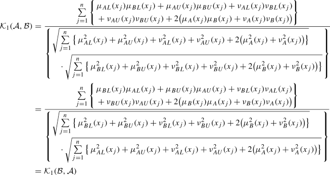
• (P2) For CIFSs ${\mathcal {A}}$ and ${\mathcal {B}}$, we have

  

• (P3) As ${\mathcal {A}}=B$, this implies that $\mu _{AL}(x_j) = \mu _{BL}(x_j)$, $\mu _{AU}(x_j) = \mu _{BU}(x_j)$, $\nu _{AL}(x_j) = \nu _{BL}(x_j)$, $\nu _{AU}(x_j) = \nu _{BU}(x_j)$, $\mu _{A}(x_j) = \mu _{B}(x_j)$ as well as $\nu _{A}(x_j) = \nu _{B}(x_j)$, for all j. Hence, ${\mathcal {K}}_1({\mathcal {A}}, {\mathcal {B}})=1$.

Example 1

Let ${\mathcal {A}}=\big \{\big (x_1, ([0.2,0.4]$, [0.3, 0.5]), $(0.3,0.4)\big )$, $\big ( x_2,([0.3,0.4]$, [0.2, 0.6]), $(0.1,0.3)\big )\big \}$ and ${\mathcal {B}}= \big \{\big (x_1, ([0.1,0.4]$, [0.2, 0.5]), $(0.2,0.3)\big )$, $\big (x_2, ([0.1,0.2]$, [0.3, 0.4]), $(0.2,0.4)\big )\big \}$ be two CIFSs defined on ${\mathcal {X}}=\{x_1,x_2\}$. Then, by Eq. (5), we get

$$\begin{aligned} E({\mathcal {A}})&= \sum \limits _{j=1}^{2}\left( \frac{\mu _{AL}^2(x_j)}{2} + \frac{\mu _{AU}^2(x_j)}{2}\right. \\&\quad \left. + \frac{\nu _{AL}^2(x_j)}{2} + \frac{\nu _{AU}^2(x_j)}{2} + \mu _{A}^2(x_j)+ \nu _{A}^2(x_j) \right) \\&= \frac{(0.2)^2}{2} + \frac{(0.4)^2}{2} + \frac{(0.3)^2}{2} + \frac{(0.5)^2}{2}\\ {}&\quad + (0.3)^2 + (0.4)^2 \\&\quad + \frac{(0.3)^2}{2}+ \frac{(0.4)^2}{2} + \frac{(0.2)^2}{2} + \frac{(0.6)^2}{2}\\&+ (0.1)^2 + (0.3)^2= 0.945. \end{aligned}$$

Similarly, we get

$$\begin{aligned} E({\mathcal {B}})&= \sum \limits _{j=1}^{2}\left( \frac{\mu _{BL}^2(x_j)}{2} + \frac{\mu _{BU}^2(x_j)}{2} + \frac{\nu _{BL}^2(x_j)}{2} + \frac{\nu _{BU}^2(x_j)}{2}\right. \\ {}&\left. \qquad +\, \mu _{B}^2(x_j)+ \nu _{B}^2(x_j) \right) \\&= \frac{(0.1)^2}{2} + \frac{(0.4)^2}{2} + \frac{(0.2)^2}{2} + \frac{(0.5)^2}{2} + (0.2)^2 + (0.3)^2 \\&\quad + \frac{(0.1)^2}{2} + \frac{(0.2)^2}{2} + \frac{(0.3)^2}{2} + \frac{(0.4)^2}{2} + (0.2)^2 + (0.4)^2 \\&= 0.71. \end{aligned}$$

Now, using Eq. (7), we have

$$\begin{aligned} {\mathcal {C}}({\mathcal {A}}, {\mathcal {B}})&= \sum \limits _{j=1}^{2} \left\{ \begin{aligned} \frac{\mu _{AL}(x_j)\mu _{BL}(x_j)}{2} + \frac{\mu _{AU}(x_j) \mu _{BU}(x_j)}{2} + \frac{\nu _{AL}(x_j)\nu _{BL}(x_j)}{2} \\ + \frac{\nu _{AU}(x_j)\nu _{BU}(x_j)}{2} + \mu _{A}(x_j) \mu _{B}(x_j)+\nu _{A}(x_j) \nu _{B}(x_j) \end{aligned} \right\} \\&= \left( \frac{0.2\times 0.1}{2}\right) + \left( \frac{0.4\times 0.4}{2}\right) + \left( \frac{0.3\times 0.2}{2}\right) + \left( \frac{0.5\times 0.5}{2}\right) + 0.3\times 0.2\\&\quad + 0.4\times 0.3 + \left( \frac{0.3\times 0.1}{2}\right) + \left( \frac{0.4\times 0.2}{2}\right) + \left( \frac{0.2\times 0.3}{2}\right) + \left( \frac{0.6 \times 0.4}{2}\right) + 0.1 \times 0.2 + 0.3\times 0.4 = 0.77. \end{aligned}$$

Thus, Eq. (8) becomes ${\mathcal {K}}_1({\mathcal {A}}, {\mathcal {B}}) = 0.9400$.

Next, by incorporating the pessimistic attitude of the experts, we define a CC ${\mathcal {K}}_2$ as below.

Definition 9

The correlation coefficient ${\mathcal {K}}_2$ between CIFSs ${\mathcal {A}}$ and ${\mathcal {B}}$ is stated as

$$\begin{aligned}&{\mathcal {K}}_2({\mathcal {A}}, {\mathcal {B}}) \!=\! \frac{{\mathcal {C}}({\mathcal {A}}, {\mathcal {B}})}{\max \{E({\mathcal {A}}), E({\mathcal {B}})\}}\!=\! \frac{\sum \limits _{j=1}^{n}\left\{ \begin{aligned}&\mu _{AL}(x_j) \mu _{BL}(x_j)+ \mu _{AU}(x_j) \mu _{BU}(x_j) + \nu _{AL}(x_j) \nu _{BL}(x_j) \\&+ \nu _{AU}(x_j) \nu _{BU}(x_j) +2\big (\mu _{A}(x_j) \mu _{B}(x_j) + \nu _{A} (x_j) \nu _{B}(x_j)\big ) \end{aligned} \right\} }{\max \left\{ \sum \limits _{j=1}^{n}\left\{ \begin{aligned} {\mu _{AL}^2(x_j)}+{\mu _{AU}^2(x_j)} + {\nu _{AL}^2(x_j)} \\ + {\nu _{AU}^2(x_j)}+ 2\big ({\mu _{A}^2(x_j)}+{\nu _{A}^2(x_j)}\big )\end{aligned}\right\} , \sum \limits _{j=1}^{n}\left\{ \begin{aligned} {\mu _{BL}^2(x_j)}+ {\mu _{BU}^2(x_j)}+ {\nu _{BL}^2(x_j)} \\ + {\nu _{BU}^2(x_j)}+ 2\big ({\mu _{B}^2(x_j)}+{\nu _{B}^2(x_j)}\big )\end{aligned}\right\} \right\} }. \end{aligned}$$

(9)

Theorem 2

The correlation coefficient ${\mathcal {K}}_2$ have the following properties : 

• (P1) $0 \le {\mathcal {K}}_2({\mathcal {A}}, {\mathcal {B}}) \le 1$.

• (P2) ${\mathcal {K}}_2({\mathcal {A}}, {\mathcal {B}})={\mathcal {K}}_2({\mathcal {B}}, {\mathcal {A}})$.

• (P3) ${\mathcal {K}}_2({\mathcal {A}}, {\mathcal {B}})=1,$ if ${\mathcal {A}}=B.$

Proof

By Cauchy–Schwarz inequality:

$$\begin{aligned}&\sum \limits _{j=1}^{n} x_j y_j \le \sqrt{\left( \sum _{j=1}^n x_j^2\right) \cdot \left( \sum _{j=1}^n y_j^2\right) }\\ {}&\le \sqrt{\left( \max \left\{ \sum _{j=1}^n x_j^2, \sum _{j=1}^n y_j^2\right\} \right) ^2} = \max \left\{ \sum _{j=1}^n x_j^2, \sum _{j=1}^n y_j^2\right\} . \end{aligned}$$

Thus, by Eq. (9), we get $0\le {\mathcal {K}}_2({\mathcal {A}}, {\mathcal {B}}) \le 1$.

Also,

To pay an attention on different expert’s importance based on weight $\xi _j>0$ with $\sum _{j=1}^n \xi _j=1$, we state weighted CC between two CIFSs as follows:

(10)

and

(11)

Remark 3

When $\xi =\big (\frac{1}{n},\frac{1}{n},\ldots ,\frac{1}{n}\big )^{\mathrm{T}}$, Eqs. (10) and (11) reduces to Eqs. (8) and (9).

Theorem 3

The measure stated in Eq. (10) have the following properties : 

• (P1) $0 \le {\mathcal {K}}_3({\mathcal {A}}, {\mathcal {B}}) \le 1$.

• (P2) ${\mathcal {K}}_3({\mathcal {A}}, {\mathcal {B}})={\mathcal {K}}_3({\mathcal {B}}, {\mathcal {A}})$.

• (P3) ${\mathcal {K}}_3({\mathcal {A}}, {\mathcal {B}})=1$, if ${\mathcal {A}}=B$.

Proof

We shall show that ${\mathcal {K}}_3({\mathcal {A}}, {\mathcal {B}}) \le 1$, while others are trial.

$$\begin{aligned} {\mathcal {C}}_w({\mathcal {A}}, {\mathcal {B}})&= \sum \limits _{j=1}^{n} \xi _j \left\{ \begin{aligned} \frac{\mu _{AL}(x_j)\mu _{BL}(x_j)}{2} + \frac{\mu _{AU}(x_j)\mu _{BU}(x_j)}{2} + \frac{\nu _{AL}(x_j)\nu _{BL}(x_j)}{2} \\ + \frac{\nu _{AU}(x_j)\nu _{BU}(x_j)}{2} + \mu _{A}(x_j) \mu _{B}(x_j)+\nu _{A}(x_j) \nu _{B}(x_j) \end{aligned} \right\} \\&= \sum \limits _{j=1}^{n} \left\{ \begin{aligned} \frac{\sqrt{\xi _j} \mu _{AL}(x_j)}{\sqrt{2}}\frac{\sqrt{\xi _j} \mu _{BL}(x_j)}{\sqrt{2}} + \frac{\sqrt{\xi _j} \mu _{AU}(x_j)}{\sqrt{2}} \frac{\sqrt{\xi _j} \mu _{BU}(x_j)}{\sqrt{2}} \\ + \frac{\sqrt{\xi _j} \nu _{AL}(x_j)}{\sqrt{2}}\frac{\sqrt{\xi _j} \nu _{BL}(x_j)}{\sqrt{2}} + \frac{\sqrt{\xi _j} \nu _{AU}(x_j)}{\sqrt{2}} \frac{\sqrt{\xi _j} \nu _{BU}(x_j)}{\sqrt{2}} \\ + \sqrt{\xi _j} \mu _{A}(x_j) \sqrt{\xi _j} \mu _{B}(x_j)+\sqrt{\xi _j} \nu _{A}(x_j) \sqrt{\xi _j} \nu _{B}(x_j) \end{aligned} \right\} . \end{aligned}$$

By Cauchy–Schwarz inequality,

$$\begin{aligned}&({\mathcal {C}}_w({\mathcal {A}}, {\mathcal {B}}))^2 \\&\quad \le \left\{ \xi _1 \left\{ \begin{aligned}\frac{\mu _{AL}^2(x_1)}{2} + \frac{\mu _{AU}^2(x_1)}{2} + \frac{\nu _{AL}^2(x_1)}{2} \\ +\frac{\nu _{AU}^2(x_1)}{2}+ \mu _{A}^2(x_1)+\nu _{A}^2(x_1) \end{aligned} \right\} \right. \\ {}&\qquad \left. + \xi _2 \left\{ \begin{aligned}\frac{\mu _{AL}^2(x_2)}{2} + \frac{\mu _{AU}^2(x_2)}{2} + \frac{\nu _{AL}^2(x_2)}{2} \\ +\frac{\nu _{AU}^2(x_2)}{2}+ \mu _{A}^2(x_2)+\nu _{A}^2(x_2) \end{aligned} \right\} \right. \\&\qquad \left. + \cdots + \xi _n \left\{ \begin{aligned} \frac{\mu _{AL}^2(x_n)}{2} + \frac{\mu _{AU}^2(x_n)}{2} + \frac{\nu _{AL}^2(x_n)}{2} \\ +\frac{\nu _{AU}^2(x_n)}{2}+ \mu _{A}^2(x_n)+\nu _{A}^2(x_1) \end{aligned} \right\} \right\} \times \\&\qquad \times \left\{ \xi _1 \left\{ \begin{aligned} \frac{\mu _{BL}^2(x_1)}{2} + \frac{\mu _{BU}^2(x_1)}{2} + \frac{\nu _{BL}^2(x_1)}{2} \\ +\frac{\nu _{BU}^2(x_1)}{2}+ \mu _{B}^2(x_1)+\nu _{B}^2(x_1) \end{aligned} \right\} \right. \\ {}&\left. \qquad +\, \xi _2 \left\{ \begin{aligned}\frac{\mu _{BL}^2(x_2)}{2} + \frac{\mu _{BU}^2(x_2)}{2} + \frac{\nu _{BL}^2(x_2)}{2} \\ +\frac{\nu _{BU}^2(x_2)}{2}+ \mu _{B}^2(x_2)+\nu _{B}^2(x_2) \end{aligned} \right\} \right. \\&\qquad \left. + \cdots + \xi _n \left\{ \begin{aligned} \frac{\mu _{BL}^2(x_n)}{2} + \frac{\mu _{BU}^2(x_n)}{2} + \frac{\nu _{BL}^2(x_n)}{2} \\ +\frac{\nu _{BU}^2(x_n)}{2}+ \mu _{B}^2(x_n)+\nu _{B}^2(x_1) \end{aligned} \right\} \right\} \\&\quad \le \sum \limits _{j=1}^n \xi _j \left\{ \begin{aligned} \frac{\mu _{AL}^2(x_j)}{2} + \frac{\mu _{AU}^2(x_j)}{2} + \frac{\nu _{AL}^2(x_j)}{2} \\ +\frac{\nu _{AU}^2(x_j)}{2}+ \mu _{A}^2(x_j)+\nu _{A}^2(x_j) \end{aligned} \right\} \\ {}&\times \sum \limits _{j=1}^n \xi _j \left\{ \begin{aligned} \frac{\mu _{BL}^2(x_j)}{2} + \frac{\mu _{BU}^2(x_j)}{2} + \frac{\nu _{BL}^2(x_j)}{2} \\ +\frac{\nu _{BU}^2(x_j)}{2}+ \mu _{B}^2(x_j)+\nu _{B}^2(x_j) \end{aligned} \right\} \\&\quad \le E_w({\mathcal {A}})\cdot E_w({\mathcal {B}}). \end{aligned}$$

Therefore, ${\mathcal {K}}_3({\mathcal {A}}, {\mathcal {B}}) \le 1$.

Decision-making approach and illustration

This section presents a decision-making approach and its illustration with several examples. To apply the proposed series of correlation coefficients in the following approach, CIFSs are considered to be corresponding to each alternative-criteria pair. This turns the indices into matrix format, where the indices for rows stand for alternative and indices for columns stand for criteria. This do not disturb the numerical applicability of the proposed correlation coefficients in Eqs. (8)–(11). The purpose of listing into matrix format is only for the convenience of the user to apply the proposed coefficients for the analysis of the various alternatives subjected under criteria information. On the basis of this, the proposed approach is set out below:

Proposed method

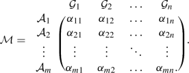
Consider a DM problem with “m” alternatives $\{{\mathcal {A}}_1, {\mathcal {A}}_2,\ldots ,{\mathcal {A}}_m\}$ and “n” criteria $\{{\mathcal {G}}_1$, ${\mathcal {G}}_2,\ldots ,{\mathcal {G}}_n\}$. Assume an expert has been assigned to evaluate each ${\mathcal {A}}_i$ under ${\mathcal {G}}_j$ and give their preferences in terms of CIFNs. The values are denoted by $\alpha _{ij} = \big (([\mu ^L_{ij},\mu ^U_{ij}]$, $[\nu ^L_{ij},\nu ^U_{ij}])$, $(\mu _{ij},\nu _{ij})\big )$ with $[\mu _{ij}^L, \mu _{ij}^U]$, $[\nu _{ij}^L, \nu _{ij}^U] \subseteq [0,1]$, $\mu _{ij}, \nu _{ij} \in [0,1]$ and $\mu _{ij}^{U} +\nu _{ij}^{U} \le 1$, $\mu _{ij} + \nu _{ij}\le 1$ for $i=1,2,\ldots ,m; j=1,2,\ldots ,n$. Let $\xi _j>0$ be the importance factor of ${\mathcal {G}}_j$ with $\sum _{j=1}^n \xi _j = 1$. Then the subsequent steps are performed to figure the most appropriate option using the proposed measures.

• Step 1: Collect the information as decision matrix $\mathcal {M}$

  

• Step 2: Take the ideal alternative ${\mathcal {A}}$ which can be considered as a reference set.

• Step 3: Utilize the proposed measures either ${\mathcal {K}}_1$ or ${\mathcal {K}}_2$ or ${\mathcal {K}}_3$ or ${\mathcal {K}}_4$ as given in Eqs. (8)–(11) to compute the measurement degrees between ${\mathcal {A}}_i$ and ${\mathcal {A}}$.

• Step 4: Order the element with index of “$\arg \max {{\mathcal {K}}}$”.

Illustrative examples

The applicability of the presented measures and method has been illustrated with several examples as below.

Example 2

Watersheds are the hydrological geographical areas which act as drainage or the area where the water is accumulated from larger bodies of water such as streams, rivers, and ponds. Watersheds mainly comprise the upper layer of flowing waters. They are mainly in the form of basins, catchments, sub-catchments, etc. These watersheds are extremely useful for saving water resources from pollution and for the efficient usage of the water resources for both domestic and professional purposes so that no harm can be caused by human interference. In-depth analysis of watershed management has shown that efficient watersheds can be assessed by a number of factors such as water quality, prospering flora and fauna, that are capable of being an emergency drought savior, etc. Focussing on the main factors associated with the efficiency of the watershed’s, the following points are outlined:

Table 1 Input preference of given watersheds

• (i) Water quality: The efficiency of watersheds’ is mainly determined by their water quality. The flowing water in the mainstream rivers, ponds etc, has accumulated in the watersheds and thus contains the upper layer of the flowing water. The purity of this upper layer of water in the watersheds ensures that it can be used for mankind purposes as well as for surrounding animals. The cleanliness of water also supports the health of other living creatures surviving in the ecosystem.

• (ii) Habitat provider: Well managed watersheds are needed, not only for the human purposes, but also for the flora and fauna in the local surroundings. The aquatic plants and animals remains healthy if the watersheds are maintained properly. So, watersheds can be served as the natural habitats for the aquatic animals and many other hydrological species. Thus, these aquatic animals such as small fishes can also be used for the economical purposes. These entrepreneurial activities provide income for the surrounding people. But this balance of aquatic life and pisciculture practices can only be achieved if the water in the water-sheds is clear and fit for life survival.

• (iii) Protection from emergent situations: Often, with seasonal fluctuations and weather conditions or due to economic conditions in a particular geographical area, emergent situations such as droughts or floods may arise. Watershed management therefore focusses on maintaining the watershed levels in such a way that they can act as a boon during the drought conditions and on the other hand, do not cause any risk during the time of floods.

• (iv) Efficient use of other associated resources: In the analysis of watershed management, the efficient use of associated resources is one of the key factors affecting more challenging situations. These associated resources are mainly including the surrounding land and water. Watersheds may have boundaries in the residential and geographical areas where human activities are carried out in a frequent manner such as watersheds around agricultural land. It may also pass through any residential area. It is therefore clear from these facts that watersheds can never be kept entirely free from human interference. There may arise situations where the boundaries of the watersheds need to be clearly highlighted in order to optimize the use of the land surrounding them. In other words, one of the main factors affecting watershed management is that there should be no exploitation of the associated resources. In watershed management, there are no forests, no land areas, no agricultural land areas and no residential areas get affected.

So, bearing in mind all of the factors mentioned above, we have set four main criteria on which the entire case study will be carried out. These associated criteria are: ‘Water quality’; ‘Habitat provider’; ‘Protection from emergency situations’ and ‘Efficient use of the associated resources’. Thus, this case study focuses on the determination of watershed management in four different watershed locations viz. ${\mathcal {B}}_1, {\mathcal {B}}_2 , {\mathcal {B}}_3$ and ${\mathcal {B}}_4$; on the outskirts of city Patiala situated in Punjab state of India. The objective of the study is to compare these watershed regions with the ideal watershed area, so in order to determine which watershed area is well managed as compared to all other. During the conduct of this analysis, the information is collected in the form of CIFSs, in which the IVIFS captures the opinion of the common person residing in that geographical region, and the corresponding IFS captures the agreement as well as disagreement with the IVIFS in accordance with the expert committee, including the board of directors with expertise in watershed management.

The standardized CIFS, called as the reference set, which is used for the correlational comparability is given as follows:

$$\begin{aligned} {\mathcal {A}} =\left\{ \begin{aligned}&\Big (x_1,\big (([0.20,0.35],[0.05,0.10]),(0.10,0.50)\big )\Big ), \Big (x_2,\big (([0.60,0.65],[0.20,0.23]),(0.20,0.40)\big )\Big ),\\&\Big (x_3,\big (([0.55,0.60],[0.18,0.21]),(0.20,0.60)\big )\Big ), \Big (x_4,\big (([0.50,0.55],[0.05,0.10]),(0.20,0.40)\big )\Big ) \end{aligned} \right\} . \end{aligned}$$

The CIFS ${\mathcal {A}}$ is checked for correlation coefficients with that of CIFSs capturing information corresponding to the locations ${\mathcal {B}}_1,$ ${\mathcal {B}}_2$ , ${\mathcal {B}}_3$ and ${\mathcal {B}}_4$. Their rating values are given in Table 1.

For a clear explanation of uncertainty handling by CIFS, we explain with the help of the CIFS corresponding to the ${\mathcal {B}}_1$ and $x_1$ entries in Table 1. Since the objective of the problem is to conclude that the watershed is more correlated with the ideal watershed, the information is gathered from local residents around the watershed (in form of IVIFS) and further the rating towards the local resident’s opinion is given by expert committee member visiting the location. For alternative ${\mathcal {B}}_1$, under the criterion $x_1$ (representing water quality), the rating provided by local residents is $\left( \left[ 0.20,0.25 \right] , \left[ 0.30,0.35 \right] \right)$, i.e., they are satisfied with the water quality between 20–25% and dissatisfied by 30–35%. However, the expert member disagrees with the stated satisfaction level of $20\%$ and agrees towards dissatisfied level of $30\%$ (R-order consideration). The detailed listing of this situation in comparison to other existing environments (IFS, IVIFS and CFS), is provided in Table 2.

Table 2 Information handling capacity of CIFSs in contrast to different environments

The indices values corresponding to ${\mathcal {K}}_1$ and ${\mathcal {K}}_2$ are estimated from set ${\mathcal {A}}$ to ${\mathcal {B}}_k$, $(k=1,2,3,4)$ as follows:

$$\begin{aligned}&{\mathcal {K}}_1({\mathcal {B}}_1, {\mathcal {A}})=0.7641; \quad {\mathcal {K}}_1({\mathcal {B}}_2, {\mathcal {A}})=0.9138; \\&{\mathcal {K}}_1({\mathcal {B}}_3, {\mathcal {A}})=0.7827; \quad {\mathcal {K}}_1({\mathcal {B}}_4, {\mathcal {A}})=0.8802 \end{aligned}$$

and

$$\begin{aligned}&{\mathcal {K}}_2({\mathcal {B}}_1, {\mathcal {A}})=0.7610; \quad {\mathcal {K}}_2({\mathcal {B}}_2, {\mathcal {A}})=0.8852; \\&{\mathcal {K}}_2({\mathcal {B}}_3, {\mathcal {A}})=0.7140; \quad {\mathcal {K}}_2({\mathcal {B}}_4, {\mathcal {A}})=0.8101. \end{aligned}$$

Thus, the ordering is ${\mathcal {B}}_2 \succ {\mathcal {B}}_4 \succ {\mathcal {B}}_3 \succ {\mathcal {B}}_1$ when ${\mathcal {K}}_1$ correlation coefficient index has been used while ${\mathcal {B}}_2 \succ {\mathcal {B}}_4 \succ {\mathcal {B}}_1 \succ {\mathcal {B}}_3$ when ${\mathcal {K}}_2$ used. If $\xi =(0.18, 0.23, 0.30, 0.29)^{\mathrm{T}}$ is taken, we get

$$\begin{aligned}&{\mathcal {K}}_3({\mathcal {B}}_1, {\mathcal {A}})=0.7643; \quad {\mathcal {K}}_3({\mathcal {B}}_2, {\mathcal {A}})=0.9166; \\&{\mathcal {K}}_3({\mathcal {B}}_3, {\mathcal {A}})=0.7844; \quad {\mathcal {K}}_3({\mathcal {B}}_4, {\mathcal {A}})=0.8986 \end{aligned}$$

and

$$\begin{aligned}&{\mathcal {K}}_4({\mathcal {B}}_1, {\mathcal {A}})=0.7623; \quad {\mathcal {K}}_4({\mathcal {B}}_2, {\mathcal {A}})=0.8687; \\&{\mathcal {K}}_4({\mathcal {B}}_3, {\mathcal {A}})=0.7196; \quad {\mathcal {K}}_4({\mathcal {B}}_4, {\mathcal {A}})=0.8088. \end{aligned}$$

Therefore, the ranking ${\mathcal {B}}_2\succ {\mathcal {B}}_4\succ {\mathcal {B}}_3 \succ {\mathcal {B}}_1$ and ${\mathcal {B}}_2\succ {\mathcal {B}}_4\succ {\mathcal {B}}_1 \succ {\mathcal {B}}_3$ obtained from measures ${\mathcal {K}}_3$ and ${\mathcal {K}}_4$. Hence, the watershed management at location ${\mathcal {B}}_2$ is more correlated with the standardized CIFS value than the remaining three locations.

Example 3

This case study focuses on the recruitment of personnel by a prominent globally recognized recruitment agency located in India.

International Manpower Resources (IMR) Private Limited, headquartered at New Delhi, India, is an organization which has been established some decades ago. It is a very need-driven initiated agency which was set up at 1990 at a time when there were frequent demands on India from the Middle East, regarding the supply of manpower. Indeed, the sudden upsurge in Middle East economic activity, due to the discovery of oil and subsequent upliftment of commerce as well as industry, has given rise to globalization. Because India was an economically cheap country compared to the Middle East countries, the labor force in India was in frequent demand. So, the establishment of the IMR was basically the outcome of the need for an professional agency to supply the manpower to the foreign lands. Thus, main working type of the IMR is the analyze of the standardized eligibility for a particular job by any country and the provision of the best-fit candidate among the Indian pool of applicants. The main work of IMR is, therefore, to access the needs of foreign clients and to make them available the prospective candidate(s). Suppose, a new client has requested for candidates to start a new project. Among the pool of applicants, the performance needs of the client are to be analyzed on the basis of four criteria $x_j$ where $j=(1,2,3,4)$ i.e. $x_1$: ‘Educational Qualification’, $x_2$ : ‘Communication Skills’, $x_3$: ‘Presentation Skills’ and $x_4$: ‘Working Speed’. Let ${\mathcal {A}}$ be the formulated desired standard set formulated as:

$$\begin{aligned} {\mathcal {A}} = \left\{ \begin{aligned}&(x_1,(([0.60,0.65],[0.05,0.10]),(0.10,0.30))), (x_2,(([0.50,0.55],[0.18,0.20]),(0.10,0.40))),\\&(x_3,(([0.45,0.50],[0.15,0.20]),(0.10,0.60))), (x_4,(([0.30,0.35],[0.18,0.20]),(0.10,0.80))). \end{aligned} \right\} . \end{aligned}$$

During the different stages of the recruitment process, four persons (${\mathcal {P}}_1, {\mathcal {P}}_2, {\mathcal {P}}_3, {\mathcal {P}}_4$) are shortlisted for personal interviews. For these persons, the interval-valued intuitionistic fuzzy judgements are obtained at the first stage of the recruitment process by the evaluator and the intuitionistic fuzzy judgements are provided by the main IMR recruitment director. The CIFS entry for candidate ${\mathcal {P}}_1$ corresponding to criterion $x_1:$ ‘Educational Qualification’ is $\left( \left( \left[ 0.30,0.40 \right] ,\left[ 0.15,0.20 \right] \right) ,\left( 0.10,0.20 \right) \right) .$ It represents that at the first stage of recruitment the expert is 30–40% in favor of selecting candidate ${\mathcal {P}}_1$ and 15–20% not in favor of the selection. However, the recruitment director of the firm disagrees $10\%$ and agrees by $20\%$ to the judgement provided by expert at the first stage. Information regarding these shortlisted candidates is formulated in the form of CIFSs as:

$$\begin{aligned}&{\mathcal {P}}_1 = \left\{ \begin{aligned}&\Big (x_1,\big (([0.30,0.40],[0.15,0.20]),(0.10,0.20)\big )\Big ), \Big (x_2,\big (([0.50,0.55],[0.20,0.30]),(0.30,0.40)\big )\Big ),\\&\Big (x_3,\big (([0.10,0.20],[0.15,0.20]),(0.10,0.15)\big )\Big ), \Big (x_4,\big (([0.20,0.25],[0.40,0.45]),(0.20,0.40)\big )\Big ) \end{aligned} \right\} \\&{\mathcal {P}}_2 = \left\{ \begin{aligned}&\Big (x_1,\big (([0.60,0.65],[0.05,0.10]),(0.15,0.30)\big )\Big ), \Big (x_2,\big (([0.30,0.32],[0.40,0.43]),(0.10,0.20)\big )\Big ), \\&\Big (x_3,\big (([0.45,0.50],[0.20,0.25]),(0.20,0.30)\big )\Big ), \Big (x_4,\big (([0.30,0.35],[0.18,0.22]),(0.10,0.30)\big )\Big ) \end{aligned} \right\} , \\&{\mathcal {P}}_3 = \left\{ \begin{aligned}&\Big (x_1,\big (([0.20,0.30],[0.15,0.20]),(0.45,0.20)\big )\Big ), \Big (x_2,\big (([0.10,0.15],[0.18,0.20]),(0.10,0.15)\big )\Big ),\\&\Big (x_3,\big (([0.30,0.33],[0.20,0.25]),(0.40,0.20)\big )\Big ), \Big (x_4,\big (([0.30,0.35],[0.40,0.42]),(0.20,0.80)\big )\Big ) \end{aligned} \right\} , \\&{\mathcal {P}}_4 =\left\{ \begin{aligned}&\Big (x_1,\big (([0.30,0.35],[0.20,0.25]),(0.50,0.30)\big )\Big ), \Big (x_2,\big (([0.20,0.23],[0.25,0.30]),(0.18,0.20)\big )\Big ),\\&\Big (x_3,\big (([0.17,0.22],[0.25,0.30]),(0.15,0.60)\big )\Big ), \Big (x_4,\big (([0.10,0.15],[0.18,0.20]),(0.10,0.30)\big )\Big ). \end{aligned} \right\} . \end{aligned}$$

The aim is to identify the best person for the reference set ${\mathcal {A}}$. For this purpose, the ${\mathcal {K}}_1$ and ${\mathcal {K}}_2$, which denotes the difference between working abilities and how close they are to the standardized ones, are computed as shown below:

$$\begin{aligned}&{\mathcal {K}}_1({\mathcal {P}}_1,{\mathcal {A}})=0.8412;\quad {\mathcal {K}}_1({\mathcal {P}}_2,{\mathcal {A}})=0.8827;\\&{\mathcal {K}}_1({\mathcal {P}}_3,{\mathcal {A}})=0.8311;\quad {\mathcal {K}}_1({\mathcal {P}}_4,{\mathcal {A}})=0.8410 \end{aligned}$$

and

$$\begin{aligned}&{\mathcal {K}}_2({\mathcal {P}}_1,{\mathcal {A}})=0.6236;\quad {\mathcal {K}}_2({\mathcal {P}}_2,{\mathcal {A}})= 0.6939; \\&{\mathcal {K}}_2({\mathcal {P}}_3,{\mathcal {A}})=0.7054;\quad {\mathcal {K}}_2({\mathcal {P}}_4,{\mathcal {A}})=0.6290. \end{aligned}$$

Thus, we conclude from their computed results that ${\mathcal {P}}_2 \succ {\mathcal {P}}_1\succ {\mathcal {P}}_4 \succ {\mathcal {P}}_3$ by ${\mathcal {K}}_1$ correlation coefficient while ${\mathcal {P}}_3 \succ {\mathcal {P}}_2 \succ {\mathcal {P}}_4 \succ {\mathcal {P}}_1$ by ${\mathcal {K}}_2$ correlation coefficient. Hence, the ranking order for the desired post has been changed as per the convenience of the decision-maker in terms of optimistic to pessimistic attitude.

Assume $\xi =(0.23,0.33,0.24,0.20)^{\mathrm{T}}$, the indices values using ${\mathcal {K}}_3$ and ${\mathcal {K}}_4$ coefficients are computed as

$$\begin{aligned}&{\mathcal {K}}_3({\mathcal {P}}_1,{\mathcal {A}})=0.8472;\quad {\mathcal {K}}_3({\mathcal {P}}_2,{\mathcal {A}})=0.8814; \\&{\mathcal {K}}_3({\mathcal {P}}_3,{\mathcal {A}})=0.8166;\quad {\mathcal {K}}_3({\mathcal {P}}_4,{\mathcal {A}})=0.8429 \end{aligned}$$

and

$$\begin{aligned}&{\mathcal {K}}_4({\mathcal {P}}_1,{\mathcal {A}})=0.6569;\quad {\mathcal {K}}_4({\mathcal {P}}_2,{\mathcal {A}})= 0.7019;\\&{\mathcal {K}}_4({\mathcal {P}}_3,{\mathcal {A}})=0.6603;\quad {\mathcal {K}}_4({\mathcal {P}}_4,{\mathcal {A}})=0.6331. \end{aligned}$$

From our analysis, we conclude that the ranking pattern is ${\mathcal {P}}_2 \succ {\mathcal {P}}_1 \succ {\mathcal {P}}_4 \succ {\mathcal {P}}_3$ by ${\mathcal {K}}_3$ and ${\mathcal {P}}_2 \succ {\mathcal {P}}_3 \succ {\mathcal {P}}_1 \succ {\mathcal {P}}_4$ by ${\mathcal {K}}_4$. Hence, by both the weighted correlation coefficients ${\mathcal {P}}_2$ remains the best-fit among all the other candidates.

Table 3 Measurement values corresponding to IFS environment

Table 4 Input data of the candidates for Example 5

Verification and comparative analysis

To generalize the capability of the CIFS with regard to the features of IVIFSs and IFSs together, we present some examples as follows.

Example 4

[32] Consider three unknown patterns ${\mathcal {A}}_1, {\mathcal {A}}_2$ and ${\mathcal {A}}_3$, which are classified under three criteria ${\mathcal {C}}_i$, $(i=1,2,3)$ under the IFS environment (a special case of CIFS environment, see Remark 2). The rating values of them are given as follows:

$$\begin{aligned} {\mathcal {A}}_1&= \{({\mathcal {C}}_1, 1.0, 0.0), ({\mathcal {C}}_2, 0.8, 0.0), ({\mathcal {C}}_3, 0.7, 0.1) \} \\ {\mathcal {A}}_2&= \{({\mathcal {C}}_1, 0.8, 0.1), ({\mathcal {C}}_2, 1.0, 0.0), ({\mathcal {C}}_3, 0.9, 0) \} \\ \text {and}\quad {\mathcal {A}}_3&= \{({\mathcal {C}}_1, 0.6, 0.2), ({\mathcal {C}}_2, 0.8, 0.0), ({\mathcal {C}}_3, 1.0, 0.0)\}. \end{aligned}$$

The optimum result is summarized in Table 3 along with existing methods [12, 32,33,34]. It is determined from this table that the most appropriate alternative achieved by the stated measures is the same and harmonizes with the existing approaches. However, the computational procedure between them is completely different. For instance, in [32, 33], the distance and similarity measures between the sets were calculated while the proposed one measured the degree of the relationship between the two sets. It is also obtained from Remark 2 that the IFS is a special case of the considered CIFS and therefore the proposed measure can equivalently handle the given IFS information. Therefore, the applicability span of the proposed method is deeper than the existing ones under the IFSs.

Example 5

[10] Consider the MCDM problem related to the manufacturing company that plans to recruit a new and efficient marketing expert. To complete this process, the company examined the six candidates ${\mathcal {A}}_i$ for the evaluation. To access these alternatives, a committee is constituted with a number of senior experts, who have taken responsibility for conducting interviews and finalizing the selection process. To further evaluation, they considered the five assessment criteria viz namely ${\mathcal {C}}_1$: “fluency in a foreign language”, ${\mathcal {C}}_2$: “oral communication skills”, ${\mathcal {C}}_3$: “emotional steadiness”, ${\mathcal {C}}_4$: “past experience” and ${\mathcal {C}}_5$: “self–confidence”. The importance of these factors are taken as $\omega =(0.05, 0.35, 0.30, 0.20, 0.1)^{\mathrm{T}}$. Under each criterion, the rating values of each candidate are assessed in terms of IVIFSs (a special case of CIFS with $(\mu , \nu )=(0,1)$ for R-order and $(\mu ,\nu )=(1,0)$ for P-order) and their decision matrix is presented in Table 4 (please see [10]).

The ranking results corresponding to this problem are listed in Table 5 along with several existing MCDM methods [10, 12, 15, 16, 32,33,34,35,36].

Table 5 shows that methods [32, 33] do not solve the MCDM problem; however, the approaches presented in [10, 15, 16, 35, 36] show that the best alternative is ${\mathcal {A}}_2$ for the required task. As the IVIFS is a special case of the considered CIFS environment (see Remark 1) by setting IFS component $(\mu ,\nu )=(0, 1)$ for the R-ordered CIFS, and therefore, the proposed measure can handle the given information accordingly. Therefore, the proposed method has wider scope than existing methods [10, 12, 15, 16, 32,33,34,35,36]. The results of the proposed measures are aligned with the results of the existing approaches under the IVIFS theories.

Example 6

[31] Consider a set of diseases ${\mathcal {Q}}= \{{\mathcal {Q}}_1$ (“Viral fever”), ${\mathcal {Q}}_2$ (“Malaria”), ${\mathcal {Q}}_3$ (“Typhoid”), ${\mathcal {Q}}_4$ (“Stomach problem”)} and a set of symptoms $\mathcal {S}=\{s_1$ (“Temperature”), $s_2$ (“Headache”), $s_3$ (“Stomach-ache”), $s_4$ (“Cough”)} and treated as an MCDM problem. Each disease is rated under the set of symptoms under the CIFS environment given in Table 6 (for more detail, see [31]).

Table 5 Comparison of ranking with different measures for Example 5

Assume a patient ${\mathcal {P}}$, whose rating values over symptoms is given as

$$\begin{aligned} {\mathcal {P}} = \left\{ \begin{aligned}&(s_1,(([0.20,0.30],[0.40,0.50]),(0.10,0.40))), (s_2,(([0.30,0.40],[0.10,0.60]),(0.20,0.40))), \\&(s_3,(([0.40,0.50],[0.20,0.30]),(0.60,0.30))), (s_4,(([0.10,0.50],[0.20,0.30]),(0.40,0.30))). \end{aligned} \right\} . \end{aligned}$$

Now, the goal is to identify the disease of patient ${\mathcal {P}}$ among ${\mathcal {Q}}_k$’s. For it, the proposed correlation measures are computed along with the existing studies [10, 12, 15, 16, 31,32,33,34,35,36], results are given in Table 7. This table shows that the methods [10, 12, 15, 16, 32,33,34,35,36] cannot solve this problem because they do not meet the conditions of IFS and IVIFS. However, the approaches under the CIFS environment [31] and the proposed method can easily handle the information. Although it can be seen that the best alternative to the problem matches the results of Garg and Kaur [31], the computational process is entirely different. In [31], the measurement values are computed from its reference sets, which shows the degree of dissimilarity between the two sets, while the stated method used considers the relationship between the sets. Also, the result show that ${\mathcal {Q}}_3$ is preferred over ${\mathcal {Q}}_2$ denoted by ${\mathcal {Q}}_3\succ {\mathcal {Q}}_2$, when ${\mathcal {K}}_1$ or ${\mathcal {K}}_3$ measurement are used, while ${\mathcal {Q}}_2\succ {\mathcal {Q}}_3$ when ${\mathcal {K}}_2$ or ${\mathcal {K}}_4$ measurement are utilized. Thus, taking advantages of the structure of these correlation coefficients, the decision makers can select and choose the alternatives based on his choices.

Table 6 Rating values for Example 6

Table 7 Measurement values corresponding to CIFS environment

Superiority analysis

The above examples show the effectiveness of the stated method; however, to elucidate the multiple advantages with the existing studies [10, 12, 15, 16, 32,33,34,35,36], we explain it in Table 8 for the considered example. In this table, the symbol $\times$ represents the failure of the environment to capture the specific environment and the symbol $\checkmark$ shows the ability of the environment over the other ones. It can be clearly seen that the approaches based on IVIFSs cannot capture the data which is available in the format of CIFSs and the decision methodologies based on IFSs cannot withstand the situations where experts provide preference values either in the form of IVIFSs or CIFSs. However, the approaches based on CIFS as that of the proposed method, captures the information can process it efficiently to rank the available alternatives w.r.t. the opted criteria values. Therefore, this analysis suggests that both the environment considered and the corresponding proposed method are more reasonable than the others. Hence, it is evident from the present study that the CIFSs inherits the ability to generalize over the existing environments.

Example 7

Consider the information mentioned in Example 2 and their results are computed with the methods [10, 12, 15, 16, 32,33,34,35,36] and presented in Table 9. From it, we conclude the ordering as ${\mathcal {B}}_2\succ {\mathcal {B}}_4\succ {\mathcal {B}}_3\succ {\mathcal {B}}_1$.

On the other hand, if we revisit Example 3 presented in “Illustrative examples” and compare the results with the approaches [10, 12, 15, 16, 32,33,34,35,36] in Table 10. To apply the existing approaches to the IVIFS environment, only the IVIF judgments were considered during the analysis and the corresponding IFS of CIFS was set as zero. On the other hand, for the implementation of the approaches [12, 32,33,34] under the IFS environment, the IVIFS judgements of each CIFS are set to be zero.

Table 8 Superiority of the considered environment in data capturing

Table 9 Values obtained on comparing with Example 2

Table 10 Values obtained on comparing with Example 3

Although the results shown in Tables 9 and 10 reveal that the optimal alternative remains the same, but the structure of the theories is entirely different. For instance, in the IFS environment, we computed the results by setting the IVIFS judgment of CIFS as a zero while for IVIFSs, we set the IFS judgment as zero. As a result, the results corresponding to them will result in some loss of information. On the other hand, the CIFS captures the two-dimensional information simultaneously and provides more detailed results of the case studies considered. However, by changing the adaptability of the IVIFSs to the IFSs, we restrict the scope of the CIFS to only one-dimensional information only. This leads to different rankings of the proposed methodology’s results as shown in Tables 9 and 10. It is, therefore, evident that the proposed methodology captures the situational aspect and delivers results by varying the analysis by means of information captured simultaneously by both IVIFSs and IFSs.

By increasing the scope of comparative studies to some notable contributions [37, 38], we are focusing on the significance of the matrix $\mathcal {M}$ considered in the proposed approach. The matrix $\mathcal {M}$ in the proposed decision-making approach is intended to show only the array representation of all the available information divided into various alternatives and criteria contemplating the CIFS information. However, the representation of the matrix $\mathcal {M}$ is the same as that of the index matrix (IM) [37] with the difference that the IM defined in [37] captures the information in the form of an IFS. The matrix $\mathcal {M}$ represented in the presented approach can be considered as an extended version of the intuitionistic fuzzy IM. However, we have not used the described operational capabilities related to IMs because our approach does not require further processing of the decision matrix. In addition, the operating capacity defined on IMs in [37] is in the form of binary operations, not unary ones, and in our approach there is no need for any matrix-centric binary operation for processing the data available in form of CIFSs.

However, the literature survey related to the suggested decision-making approaches leads us to a joint-contribution [38] by Atanassov et al. has used the concept of index matrices in decision-making approaches. On careful analysis of their proposed methodology towards the decision-making procedure has shown that the concept of index matrices and the related approach [38] can be well used in case of group decision-making. Apparently, in the group decision-making process, more than one decision matrix in the index matrix is acquired, which can be further processed using the related operations. Nevertheless, we do not question their applicability or significance, but at the same time, our approach differs in that it is not based on group decision-making. In the proposed approach, because of single decision matrix under analysis, our approach is having complete different decision-framing process than that of Atanassov et al. [38]’s approach. It is, therefore, obvious that, in contrast, to Atanassov et al. [38], the proposed methodology is efficient in handling preference ratings in format of CIFSs.

Characteristic comparison

The feature characteristics of the different methods [10, 12, 15, 16, 32,33,34,35,36] and the stated method are tabulated in Table 11. From this table, we have obtained the following information.

• (1) The symbol ‘$\checkmark$’ indicates that the associated approach provides the facility to consider the hybrid information, allows for two-dimensional information to be considered, provides generalization beyond the associated existing environments and gives freedom to choose between the optimistic as well as pessimistic behavior while conducting the decision making analysis.

• (2) The ‘$\times$’ symbol shown in the table depicts that the corresponding method and approaches given in [10, 12, 15, 16, 32,33,34,35,36] do not consider the hybrid information content as they can deal with only one environment at a time and that can be either an IVIFS or an IFS environment. It also depicts that these theories do not allow the decision maker to capture two-dimensional information covering two separate situational aspects that vary over different time intervals, nor does it provide any generalized aspect of any of the existing environment.

• (3) Covering the aspect of choice in relation to optimism and pessimism, it is noted that [10, 15, 35] approaches provide flexibility in opting for any one of the analytical patterns, while the proposed methodology allows the decision-maker to take decisions on all of these key aspects.

Table 11 Characteristic comparison of the stated method

Advantages of the proposed measure

Based on the study conducted and the comparison, we will address the subsequent benefits of the suggested method for resolving the DMPs in the CIFS environment.

• (a) The CIFS environment is considered to handle more information and to covers a wide range of areas for dealing with uncertain information, taking both IFSs and IVIFSs into a single platform. Thus, there is less loss of information in this set.

• (b) The existing CCs under the IVIFS [14, 15] and under IFS [12, 13, 19] are considered to be a special case of the proposed CCs. In addition, it is noted from the examples mentioned above that the proposed CCs handle more information than these existing ones.

• (c) The stated method contains much more information than the existing methods in the IVIFS, IFS environment, for dealing with data uncertainties. In it, the object-related information is stated more correctly and precisely. Therefore, it is a valuable tool for managing the imprecise and enigmatic knowledge during the decision-making process.

Conclusion

The CIFS is one of the prosperous continuations of the IFS, in which a range of the disagreement (in the form of IFS values) in comparison with the agreed interval region (in form of IVIFS) has been practiced in the interpretation of the data. In this manuscript, we used the CIFS environment to infer novel correlation coefficients and, therefore, a decision-making approach based on it is framed. The main advantages of the proposed work are summarized as

• (1) There is simultaneous consideration of IVIFS and IFS information encapsulated in a single CIFS. This ensures that detailed information is captured with less computational time and minimal information loss.

• (2) Four different CCs ${\mathcal {K}}_1$, ${\mathcal {K}}_2$, ${\mathcal {K}}_3$ and ${\mathcal {K}}_4$ are formulated to capture the relationship between two CIFSs. In addition, a detailed scrutiny of their applicability is carried out in two different fuzzy environments, i.e., IVIFS and IFS. It set out the concept of robustness of the proposed CCs.

• (3) The proposed CCs cover the generalized aspect of both the IVIFSs and IFSs measures. The information in the IVIFS and IFS formats can, therefore, also be handled efficiently by the given CCs. This clearly signifies that the proposed CCs will be better able to process information without compromising the original type of information available.

• (4) The approach has inborn advantages of facilitating the practitioners to solve various problems based on different situations of real-life information capture. The experts may opt for optimistic/pessimistic behavior and can achieve the desired results accordingly.

On the basis of these advantages, in this manuscript, the proposed CCs are made undergone a rigorous comparison and verification analysis which reveals that the proposed approach largely encompasses more evaluation reports on alternatives by examining both the IVIFSs and IFSs at the same time, while the existing procedures comprise either IFS or IVIFS. Some of the features of the proposed coefficients have also been studied. Finally, on the basis of these CCs, a decision-making approach has been adopted in the context of the CIFS environment. A detailed comparative study is being conducted to test the viability and applicability of the proposed approach. Thus, we conclude that the proposed methodology can effectively capture the uncertain information and guarantees robustness. In future, the outcome of this article may be extended to a number of other real-life problems such as supplier selection, recognition of patterns, and allocation of resources [39,40,41,42,43,44,45].

References

Zadeh LA (1965) Fuzzy sets. Inf Control 8:338–353
Atanassov KT (1986) Intuitionistic fuzzy sets. Fuzzy Sets Syst 20(1):87–96
Atanassov K, Gargov G (1989) Interval-valued intuitionistic fuzzy sets. Fuzzy Sets Syst 31:343–349
Garg H (2020) New ranking method for normal intuitionistic sets under crisp, interval environments and its applications to multiple attribute decision making process. Complex Intell Syst 6(3):559–571
Xu Z, Chen J (2007) Approach to group decision making based on interval valued intuitionistic judgment matrices. Syst Eng Theory Pract 27(4):126–133
Xu ZS (2007) Intuitionistic fuzzy aggregation operators. IEEE Trans Fuzzy Syst 15:1179–1187
Xu ZS, Yager RR (2006) Some geometric aggregation operators based on intuitionistic fuzzy sets. Int J Gen Syst 35:417–433
Garg H, Arora R (2020) TOPSIS method based on correlation coefficient for solving decision-making problems with intuitionistic fuzzy soft set information. AIMS Math 5(4):2944
Xue Y, Deng Y, Garg H (2021) Uncertain database retrieval with measure-based belief function attribute values under intuitionistic fuzzy set. Inf Sci 546:436–447
Dugenci M (2016) A new distance measure for interval valued intuitionistic fuzzy sets and its application to group decision making problems with incomplete weights information. Appl Soft Comput 41:120–134
Garg H, Rani D (2020) Generalized geometric aggregation operators based on t-norm operations for complex intuitionistic fuzzy sets and their application to decision-making. Cogn Comput 12(3):679–698
Ye J (2010) Fuzzy decision-making method based on the weighted correlation coefficient under intuitionistic fuzzy environment. Eur J Oper Res 205(1):202–204
Gerstenkorn T, Manko J (1991) Correlation of intuitionistic fuzzy sets. Fuzzy Sets Syst 44:39–43
Bustince H, Burillo P (1995) Correlation of interval-valued intuitionistic fuzzy sets. Fuzzy Sets Syst 74:237–244
Park DG, Kwun YC, Park JH, Park IY (2009) Correlation coefficient of interval-valued intuitionistic fuzzy sets and its application to multi attribute group decision making problems. Math Comput Model 50:1279–1293
Xu Z (2007) On similarity measures of interval-valued intuitionistic fuzzy sets and their application to pattern recognitions. J Southeast Univ 27(1):139–143
Garg H, Kaur G (2020) A robust correlation coefficient for probabilistic dual hesitant fuzzy sets and its applications. Neural Comput Appl 32(13):8847–8866
Garg H (2018) Novel correlation coefficients under the intuitionistic multiplicative environment and their applications to decision-making process. J Ind Manag Optim 14(4):1501–1519
Garg H, Kumar K (2018) A novel correlation coefficient of intuitionistic fuzzy sets based on the connection number of set pair analysis and its application. Sci Iran E 25(4):2373–2388
Jun YB, Kim CS, Yang KO (2012) Cubic sets. Ann Fuzzy Math Inform 4(1):83–98
Khan M, Abdullah S, Zeb A, Majid A (2016) Cubic aggregation operators. Int J Comput Sci Inf Secur 14(8):670–682
Mahmood T, Mehmood F, Khan Q (2017) Some generalized aggregation operators for cubic hesitant fuzzy sets and their applications to multi criteria decision making. J Math 49(1):31–49
Gulistan M, Khan S (2020) Extentions of neutrosophic cubic sets via complex fuzzy sets with application. Complex Intell Syst 6:309–320
Kaur G, Garg H (2018) Multi-attribute decision-making based on Bonferroni mean operators under cubic intuitionistic fuzzy set environment. Entropy 20(1):65. https://doi.org/10.3390/e20010065
Garg H, Kaur G (2019) Cubic intuitionistic fuzzy sets and its fundamental properties. J Mult Valued Log Soft Comput 33(6):507–537
Muneeza Abdullah S (2020) Multicriteria group decision-making for supplier selection based on intuitionistic cubic fuzzy aggregation operators. Int J Fuzzy Syst 2:810–823
Miyamoto S (2000) Multisets and fuzzy multisets. In: Liu ZQ, Miyamoto S (eds) Soft computing and human-centered machines. Computer Science Workbench. Springer, Tokyo. https://doi.org/10.1007/978-4-431-67907-3_2
Yager RR (1986) On the theory of bags. Int J Gen Syst 13(1):23–37
Kaur G, Garg H (2019) Generalized cubic intuitionistic fuzzy aggregation operators using t-norm operations and their applications to group decision-making process. Arab J Sci Eng 44(3):2775–2794
Garg H, Kaur G (2020) Extended TOPSIS method for multi-criteria group decision-making problems under cubic intuitionistic fuzzy environment. Sci Iran 27(1):396–410
Garg H, Kaur G (2020) Novel distance measures for cubic intuitionistic fuzzy sets and their applications to pattern recognitions and medical diagnosis. Granul Comput 5(2):169–184
Song Y, Wang X, Lei L, Xue A (2014) A new similarity measure between intuitionistic fuzzy sets and its application to pattern recognition. Abstr Appl Anal 2014, Article ID 384241
Boran FE, Akay D (2014) A biparametric similarity measure on intuitionistic fuzzy sets with applications to pattern recognition. Inf Sci 255:45–57
Szmidt E, Kacprzyk J, Bujnowski P (2012) Correlation between intuitionistic fuzzy sets: some conceptual and numerical extensions. In: 2012 IEEE international conference on fuzzy systems. IEEE, pp 1–7. https://doi.org/10.1109/FUZZ-IEEE.2012.6250832
Wei GW, Wang HJ, Lin R (2011) Application of correlation coefficient to interval-valued intuitionistic fuzzy multiple attribute decision-making with incomplete weight information. Knowl Inf Syst 26(2):337–349
Zhang Y, Ma P, Su X, Zhang C (2011) Entropy on interval-valued intuitionistic fuzzy sets and its application in multi-attribute decision making. In: 14th IEEE international conference on information fusion, pp 1–7
Atanassov KT (2014) Index matrices: towards an augmented matrix calculus, vol 573. Studies in computational intelligence book series. Springer
Atanassov K, Pasi G, Yager RR (2005) Intuitionistic fuzzy interpretations of multi criteria multi person and multi-measurement tool decision making. Int J Syst Sci 36(14):859–868
Garg H (2020) Linguistic interval-valued Pythagorean fuzzy sets and their application to multiple attribute group decision-making process. Cogn Comput 12(6):1313–1337. https://doi.org/10.1007/s12559-020-09750-4
Garg H, Kaur G (2020) Quantifying gesture information in brain hemorrhage patients using probabilistic dual hesitant fuzzy sets with unknown probability information. Comput Ind Eng 140:106211. https://doi.org/10.1016/j.cie.2019.106211
Jin F, Garg H, Pei L, Liu J, Chen H (2020) Multiplicative consistency adjustment model and data envelopment analysis-driven decision-making process with probabilistic hesitant fuzzy preference relations. Int J Fuzzy Syst 22:2319–2332
Talukdar P, Goala S, Dutta P, Limboo B (2020) Fuzzy multicriteria decision making in medical diagnosis using an advanced distance measure on Linguistic Pythagorean fuzzy sets. Ann Optim Theory Pract 3(4):113–131. https://doi.org/10.22121/AOTP.2020.250858.1044
Rahman K, Sanan A, Saleem A, Muhammad YK (2020) Some induced generalized Einstein aggregating operators and their application to group decision-making problem using intuitionistic fuzzy numbers. Ann Optim Theory Pract 3(3):15–49. https://doi.org/10.22121/AOTP.2020.241689.1036
Mittal K, Jain A, Vaisla KS, Castillo O, Kacprzyk J (2020) A comprehensive review on type 2 fuzzy logic applications: past, present and future. Eng Appl Artif Intell 95:103916
Cuevas F, Castillo O, Cortes P (2020) Towards a control strategy based on type-2 fuzzy logic for an autonomous mobile robot. In: Hybrid intelligent systems in control, Pattern recognition and medicine. Springer, Cham, pp 301–314. https://doi.org/10.1007/978-3-030-34135-0_21
Author information
Authors and Affiliations
Corresponding author
Ethics declarations
Conflict of interest
The authors declare that they have no conflict of interest.
Additional information
Publisher's Note
Springer Nature remains neutral with regard to jurisdictional claims in published maps and institutional affiliations.
Rights and permissions
Open Access This article is licensed under a Creative Commons Attribution 4.0 International License, which permits use, sharing, adaptation, distribution and reproduction in any medium or format, as long as you give appropriate credit to the original author(s) and the source, provide a link to the Creative Commons licence, and indicate if changes were made. The images or other third party material in this article are included in the article’s Creative Commons licence, unless indicated otherwise in a credit line to the material. If material is not included in the article’s Creative Commons licence and your intended use is not permitted by statutory regulation or exceeds the permitted use, you will need to obtain permission directly from the copyright holder. To view a copy of this licence, visit http://creativecommons.org/licenses/by/4.0/.
About this article
Cite this article
Garg, H., Kaur, G. Algorithm for solving the decision-making problems based on correlation coefficients under cubic intuitionistic fuzzy information: a case study in watershed hydrological system. Complex Intell. Syst. 8, 179–198 (2022). https://doi.org/10.1007/s40747-021-00339-4
Received:
Accepted:
Published:
Issue Date:
DOI: https://doi.org/10.1007/s40747-021-00339-4