
Abstract
Floods are multidimensional phenomena which are conventionally studied considering the pairwise dependence between peak flow and flood volume or peak flow and duration. In this paper, the flood phenomenon is analysed based on the peak flow-flood volume dependence. The paper presents a comparison between two methodologies for the double frequency analysis using a bivariate probability distribution and the copulas approach. The comparison is performed with data from a case study example of the Ashuapmushuan river basin in Quebec, Canada. In the presented example the bivariate Extreme Value distribution type I (Gumbel) is used for comparison with the bivariate Gumbel-Hougaard Archimedean copula. For the parameters estimation of the the latter, the Kendall method and the maximum likelihood method are employed. Based on the derived results of the analysed example, it can be concluded that for engineering purposes, the copulas approach, regardless of the method of its parameter estimation, provides a simple and accurate approach for the frequency analysis of floods and the estimation of the design variables thereof. The Kendall estimation parameter method, as simpler method, is easier to apply.
1 Introduction
Most of the extreme natural hazardous phenomena can be comprehensively described as multidimensional phenomena. Attributes such as intensity, total magnitude, duration and timing of each extreme event are required to quantify fully the severity and destructive capacity of each such phenomenon (Goel et al. 1998; De Michele et al. 2004).
As known, hazard is defined as a source of potential harm, a situation with the potential to cause damage, or a threat/condition with the potential to create loss of lives or to initiate a failure to the natural, modified or human systems (Tsakiris 2007, 2014). For this purpose detailed flood simulation models in complex environments are required (Tsakiris and Bellos 2014; Bellos and Tsakiris 2015).
To account for the possible damages, losses and fatalities of each hazard event, the hazard magnitude should be transmitted through the affected system’s vulnerability (incorporating exposure), so that the risk of the affected system is estimated (Pistrika et al. 2014).
In this effort, it is of outmost importance to describe the magnitude of the extreme event with some of its essential characteristics. Focusing on flood events, it may be concluded that at least the peak flow and the volume or the peak flow and the duration are required for a realistic description of each event.
Since flood events can occur in different times with different magnitudes/intensities, the entire flood hazard can be, therefore, described by a time series of two dimensional events. The nature of this timeseries is stochastic in general. However, in most cases, it can be also regarded as a realisation of a random process, provided that its cause is totally natural. This means that in practice at least a two-dimensional probabilistic analysis is required.
It is to note, however, that in engineering practice, for simplicity purposes, the most common approach is to use a univariate probability analysis which concentrates on the peak intensity of the phenomenon (peak flow). This simplistic approach, however, cannot be applied to affected systems with storage facilities (natural and technical), in which the flood volume may be more critical than the peak flow.
These thoughts lead to the conclusion that at least the bivariate probabilistic analysis, including peak flow and volume, is necessary for all flood engineering design and management problems (Shiau 2003; Goodarzi et al. 2011). For this purpose, if both variates follow the same probability distribution, the analysis can be performed using the corresponding bivariate probability distribution (Gumbel and Mustafi 1967). That is, if peak flow and volume follow the Extreme Value distribution Type I, known as Gumbel distribution, the probability distribution for the simultaneous frequency analysis of both variates is the bivariate Gumbel distribution (Yue 2000).
Apparently there are cases in which the two variates follow different (marginal) probability distributions. In this case, the above approach cannot be followed. As a solution to this case the method of copulas can be employed.
Several authors have published hydrological studies based on the method of copulas. To mention some of these studies from a long list of studies, we can refer to Genest and Favre (2007), Salvadori et al. (2007) and many others. Storms, floods and droughts are among the phenomena analysed using the method of copulas (Shiau 2003, 2006; Huang et al. 2015).
It is the objective of this paper to prove, through the analysis of a real world case study with annual maxima of peak flow and flood volume, the usefulness of the method of copulas mainly for the design and management of flood defence engineering projects.
The data selected were first tested for the assumption that both variates, separately, follow the Gumbel distribution. For this purpose the available timeseries of annual maxima of peak flow and volume were analysed by both approaches: the bivariate Gumbel distribution and the Archimedean Gumbel-Hougaard bivariate copula. Then, the results from these methods were compared in terms of the derived return period which takes into account both the interrelated variables. Needless to say that the comparison was possible due to the assumption that the data series of both variables follow the Gumbel distribution (marginal distribution).
2 Calculation of Return Period Using the Bivariate Gumbel Distribution
Extreme event variables such as annual maximum peak flow or maximum flood volume may be studied as random variables which follow the Gumbel distribution or Extreme Value type I (EV I) distribution. A bivariate distribution is a combined distribution of two (continuous and/or discrete) marginal distributions. The joint cumulative distribution function of the Gumbel bivariate model was originally proposed by Gumbel (Gumbel and Mustafi 1967). The overall composition of the Gumbel bivariate model with standard Gumbel marginal distributions was used by many researchers in various hydrological applications. Among them Yue et al. (1999) used the bivariate Gumbel model for bivariate flood frequency analysis, and, Yue (2000) for bivariate storm frequency analysis. The bivariate Gumbel model can be expressed as:
where F(Q) and F(V) are the marginal Gumbel distribution functions of the random variables Q and V, and θ is a parameter representing the correlation between the two random variables.
The F(Q) and F(V) are written as
where α and α’ are the scale parameters, and β and β′ the location parameters of the Gumbel (EV I) distribution, for flow peak and flood volume, respectively.
The F(Q,V) is the joint probability distribution of the two random variables and parameter θ can be calculated as follows (Oliveria 1975):
where ρ is the product-moment correlation coefficient given by:
The Gumbel bivariate model can be applied to positively associated random variables with coefficient correlation less than or equal to \( \raisebox{1ex}{$2$}\!\left/ \!\raisebox{-1ex}{$3$}\right. \), limited by the parameter θ and its assessment. If ρ = 0, then θ = 0 which means that the variables Q and V are independent. In this case F(Q, V) = F(Q) ⋅ F(V). On the other hand if \( \rho =\raisebox{1ex}{$2$}\!\left/ \!\raisebox{-1ex}{$3$}\right. \), then the correlation parameter reaches its upper limit and is equal to 1 (θ = 1). Finally, if \( \rho >\raisebox{1ex}{$2$}\!\left/ \!\raisebox{-1ex}{$3$}\right. \), Eq. 4 cannot be used. This indeed is a substantial drawback of the method which limits its general application.
In the flood frequency analysis using annual maximum data, the return period T is related to the non-exceedance probability. The relationship between the non-exceedance probability and the joint return period T QV for which Q ≥ Q T or V ≥ V T can be represented by
The T QV (OR), known as «OR» return period, is very useful for the determination of design variables in flood defence projects and flood management activities since it takes account of both critical variables and their interdependence.
Other return periods such as this resulted for Q ≥ Q T and V ≥ V T , known as the «AND» return period, can be also calculated. However, return periods of this type have limited use in engineering applications.
3 Calculation of the Return Period Using an Archimedean Copula
3.1 The Archimedean Copulas
The Archimedean copulas represent a fundamental family of copulas and are often used in hydrological applications. The Archimedean copulas are quite popular due to the simplicity they offer. They have a simple form with properties such as associativity and have different dependence structures (Nelsen 1999; Genest and Rivest 1993). Many families with good properties can be derived from them. Archimedean copulas have closed-form expressions and are derived from multivariate distribution functions using Sklar’s Theorem (Salvadori et al. 2007). The Archimedean copulas can be applied to both positive and negative correlation between the variables (Genest and Favre 2007).
In order to express Archimedean copulas of two random variables X and Y, their cumulative distribution functions (CDF) F X (x), F Y (y) are set u = F X (x), v = F Y (y). Then u and v are uniformly distributed random variables. If ϕ(⋅) is the generator of Archimedean copula that is a continuous, strictly decreasing function of [0,1] to [0,∞), then the bivariate copula is defined as (Nelsen 1999):
By choosing the functions that can serve as generators, several important families of copulas are derived and can be found in the literature. The Gumbel-Hougaard copula can be considered as the representation of the bivariate distribution of extreme values. Due to this feature, the Gumbel-Hougaard Archimedean copula is likely to be the most suitable copula for multivariable hydrological frequency analysis for extreme hydrological events. It should be noted that the Gumbel-Hougaard copula can be applied when the dependence structure between the random variables is positive.
Consider the function ϕ(t) = (−ln t)θ where θ ≥ 1. The function ϕ(t) is continuous and ϕ(1) = 0. Therefore \( {\phi}^{\prime }(t)=-\theta {\left(- \ln t\right)}^{\theta -1}\frac{1}{t} \) and ϕ(t) is strictly decreasing function [0, 1] → [0, ∞]. The ϕ″(t) ≥ 0 in the interval [0,1], and therefore the ϕ is convex.
The composition of this family is expressed as:
\( {c}_{\theta}\left(u,v\right)={C}_{\theta}\left(u,v\right)\cdot \frac{{\left[\left(- \ln u\right)\cdot \left(- \ln v\right)\right]}^{\theta -1}}{u\cdot v}\cdot {\left[{\left(- \ln u\right)}^{\theta }+{\left(- \ln v\right)}^{\theta}\right]}^{\frac{2}{\theta }-2}\cdot \left\{\left(\theta -1\right)\right.\cdot {\left[{\left(- \ln u\right)}^{\theta }+{\left(- \ln v\right)}^{\theta}\right]}^{-\frac{1}{\theta }}+\left.1\right\} \)where c θ stands for the density function of the copula C θ
Furthermore, as it occurs with other couplings, the Archimedean couplings are continuous functions and decreasing for each variable, while clogged from Fréchet limits, so that the following inequality is satisfied:
3.2 Kendall Method for the Parameter Estimation
For each bivariate Archimedean copula, the value θ can be determined based on the mathematical relationship between the Kendall correlation coefficient and the generator function.
The correlation coefficient of Kendall τ can be written:
The joint cumulative probability distribution is then written:
The relationship between the non-exceedance probability and the joint return period T QV for which Q ≥ Q T or V ≥ V T can be represented as previously (Eq. 7).
3.3 The Maximum Likelihood Method for the Parameter Estimation
A second method for estimating the parameter θ of the Gumbel-Hougaard copula is the method of the maximum likelihood.
The joint p.d.f. is written:
where
Also
in which F(Q), F(V) are from Eqs. (2) and (3), respectively.
According to the above, the joint probability density function becomes:
For the estimation of θ, it is more convenient to work with the natural logarithm of the likelihood function as follows:
where ln L C is the log-likelihood function of copulas.
Then the function ln L C is maximised by setting its first derivative equal to zero. This is equivalent to setting the first derivative of the probability density function (Eq. 21) equal to zero. The solution of the latter equation (in most cases by trial and error) leads to the estimation of θ.
4 Case Study
The data used in this study were derived from the work of Yue et al. (1999). The data refer to the annual peak flows and maximum flood volumes of the Ashuapmushuan river basin of the Sagnenay region of Quebec, Canada, for the period 1963–1995. These data were used by Yue et al. (1999) in a flood frequency analysis application using the Gumbel bivariate model.
Both data series of annual maxima of peak flows and volumes are presented in Figs. 1 and 2, respectively. According to the statistical analysis of Yue et al. (1999) both series, independently considered, follow the Gumbel distribution satisfactorily, as concluded by the chi-square tests performed for this purpose. This means that the bivariate Gumbel distribution can be selected for the simultaneous frequency analysis of both peak flow and maximum flood volume. It is to be noted that in the majority of years peak flow and maximum flood volume belong to the same event. The floods of Ashuapmushuan river occur mainly in Spring and are produced due to the snow melt.

Annual peak flows of Ashuapmushuan river

Annual maxima of flood volumes of Ashuapmushuan river
Three series of calculations were performed for deriving the joint probability distribution and the «OR» return period in relation to the flood magnitudes of flow Q and volume V. The three series of calculations correspond to:
-
a)
the bivariate Gumbel probability distribution
-
b)
the 2-Copula Gumbel-Hougaard in which θ is estimated by the Kendall method
-
c)
the 2-Copula Gumbel-Hougaard with θ estimated by the maximum likelihood method.
The calculations for the bivariate Gumbel model were performed and simply coincide with the results of Yue et al. (1999). They are not presented here but they can be found in the original paper. The results can be used for comparison purposes with the above methods of Archimedean copulas (items b and c).
For the Kendall method, τ is calculated equal to 0.40909, and therefore, θ is estimated as equal to 1.692. In case θ is estimated by the maximum likelihood method, θ = 1.651 which is very close to that estimated by the Kendall method.
The results are presented in a graphical form as follows:
-
a)
2-Copula Gumbel-Hougaard/Kendall method: Joint probability distribution (Fig. 3), «OR» return period (Fig. 4)
Fig. 3 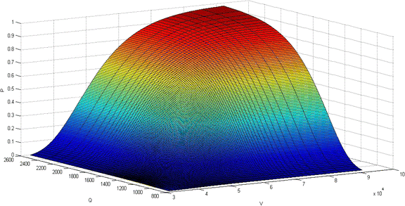
The 3D representation of the joint probability function with the Copula Gumbel-Hougaard and θ estimated by the Kendall method
Fig. 4 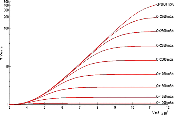
The «OR» return period as a function of peak flow and flood volume as estimated by the Gumbel-Hougaard copula with θ based on the Kendall method
-
b)
2-Copula Gumbel-Hougaard/Max likelihood method: Joint probability distribution (Fig. 5), «OR» return period (Fig. 6).
Fig. 5 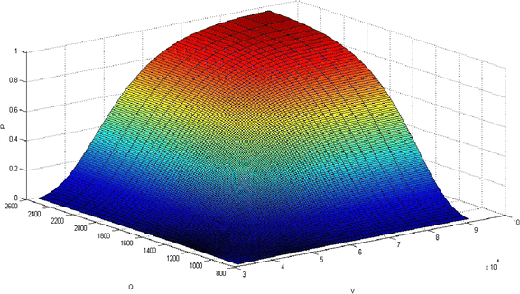
The 3D representation of the joint probability distribution with the Gumbel-Hougaard copula and θ estimated by the maximum likelihood method
Fig. 6 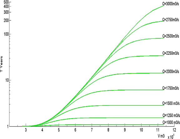
The «OR» return period as a function of peak flow and flood volume as estimated by the Gumbel-Hougaard copula with θ estimation based on the maximum likelihood method


From Figs. 3, 4, 5 and 6, it may be concluded that the results from all the three alternative methods are very close. In fact, for practical applications, they may be considered identical as can be seen from Fig. 7 in which the results from all the above mentioned alternative methods have been plotted on the same diagram for the estimation of the «OR» return periods.

The «OR» return period as a function of peak flow and flood volume as estimated by the Gumbel bivariate distribution, and the Gumbel-Hougaard copula with θ estimated by both the Kendall and the maximum likelihood methods
Although the comparison is based on a single case study, it can be supported that the method of copulas can be successfully used in case of double frequency analysis problems aiming at establishing the «OR» return period. In particular the method of copulas is useful if the marginal probability distributions are not from the same family, since in this case the bivariate distributions, such as the bivariate Gumbel distribution, cannot be used.
Finally, the method of Kendall proved successful for the estimation of the critical parameter θ and most likely can be widely used as simpler method than the maximum likelihood method. However, although in the case study analysed, both the Kendall and the maximum likelihood method produced nearly identical results for the «OR» return period, substantial deviations were observed in the estimation of the «AND» return period.
5 Concluding Remarks
Flood events are comprehensively studied taking into account their multidimensional structure. Conventionally, they are studied considering the dependence between peak flow and flood volume. By adopting the two dimensional character of floods, a double frequency analysis is performed in order to estimate the design values for the flood protection works.
The paper presented a comparison between two methodologies for the double frequency analysis: a) a bivariate probability distribution and b) the copulas approach. The comparison was performed, employing data from a case study of Ashuapmushuan river, and using the bivariate Extreme Value distribution type I (Gumbel) versus the bivariate Gumbel-Hougaard Archimedean copula.
Based on the results obtained from this case study, it can be concluded that for most flood engineering design purposes, the copula approach, provides a simple, accurate and more general approach for the frequency analysis of floods. Further, based on the single case study analysed, it is shown that the results concerning the «OR» return period are practically identical for the two methods of parameter estimation of the selected copula; that is for the maximum likelihood method and the Kendall τ method. The Kendall method, being simpler to use, is proposed for the double frequency analysis of flood events within the frame of the copula approach for engineering applications.
In the case examined, the bivariate Gumbel model results also in nearly identical «OR» return periods compared to those of copula approach. This method, however, cannot be generally used due to the existing limitations related to the marginal distributions of the involved variates.
It should be stressed that these findings, however, are derived from a single case study. To generalise these conclusions, the findings should be further verified for a large number of cases covering a wide range of values of both peak flow and flood volume.
References
Bellos V, Tsakiris G (2015) Comparing various methods of building representation for 2D-flood modelling in built-up areas. Water Resour Manag 29(2):379–397
De Michele C, Salvadori G, Canossi M, Pectaccia A, Rosso R (2004) Bivariate statistical approach to check adequacy of dam spillway. J Hydrol Eng 10(1):50–57
Genest C, Favre A (2007) Everything you always wanted to know about copula modeling but were afraid to ask. J Hydrol Eng 347-366
Genest C, Rivest L-P (1993) Statistical inference procedures for bivariate Archimedean copulas. J Am Stat Assoc 88:1034–1043
Goel NK, Seth SM, Chandra S (1998) Multivariate modeling of flood flows. J Hydraul Eng 124(2):146–155
Goodarzi E, Mirzaei M, Shui LT, Ziaei M (2011) Evaluation dam overtopping risk based on univariate and bivariate flood frequency analysis. Hydrol Earth Syst Sci Discuss 8:9757–9796
Gumbel E, Mustafi C (1967) Some analytical properties of bivariate extreme distributions. J Am Stat Assoc 62:569–588
Huang S, Chang J, Huang Q, Chen Y, Xie Y (2015) Copulas-based drought evolution characteristics and risk evaluation in a typical arid and semi-arid region. Water Resour Manag. doi:10.1007/s11269-014-0889-3
Nelsen RB (1999) An introduction to Copulas. Springer, Berlin
Oliveria J (1975) Bivariating extremes extensions. Bull Int Stat Inst 46(2):241–251
Pistrika A, Tsakiris G, Nalbantis I (2014) Flood depth-damage functions for built environment. Environ Processes 1(4):553–572
Salvadori G, De Michele C, Kottegoda NT, Rosso R (2007) Extremes in nature. An approach using Copulas, water science and technology library. Springer
Shiau JT (2003) Return period of bivariate distributed extreme hydrological events. Stoch Env Res Risk A 17:42–57
Shiau JT (2006) Fitting drought duration and severity with two dimensional copulas. Water Resour Manag 20:795–815
Tsakiris G (2007) Practical application of risk and hazard concepts in proactive planning. Eur Water 19(20):47–56
Tsakiris G (2014) Flood risk assessment: concepts, modelling, applications. Nat Hazards Earth Syst Sci 14:1361–1369
Tsakiris G, Bellos V (2014) A numerical model for two-dimensional flood routing in complex terrains. Water Resour Manag 28(5):1277–1291
Yue S (2000) The Gumbel mixed model applied to storm frequency analysis. Water Resour Manag 14:377–389
Yue S, Ouarda T, Bobee B, Legendre P, Bruneau P (1999) The Gumbel mixed model for flood frequency analysis. J Hydrol 226:88–100
Acknowledgments
The authors wish to thank the Editor and the two reviewers for their constructive comments and suggestions.
Author information
Authors and Affiliations
Corresponding author
Rights and permissions
About this article

Cite this article
Tsakiris, G., Kordalis, N. & Tsakiris, V. Flood Double Frequency Analysis: 2D-Archimedean Copulas vs Bivariate Probability Distributions. Environ. Process. 2, 705–716 (2015). https://doi.org/10.1007/s40710-015-0078-2
Received:
Accepted:
Published:
Issue Date:
DOI: https://doi.org/10.1007/s40710-015-0078-2