
Abstract
This paper analyzes the sensitivity of high-frequency radiation scattering in particulate media, to particle surface roughness. Ray-tracing theory and computation are employed. Since the magnitude of the Poynting vector ray, the irradiance, is the appropriate quantity to be tracked, the behavior of the reflectance, which controls the ratio of the reflected and incident Poynting vector magnitudes, is of primary concern. The reflectance is a highly nonlinear function of the refractive indices and angle of incidence. The present work first addresses the relationship between a single scatterer’s sensitivity to its surface roughness and then the response of a large number of scatterers to the surface roughness. The analysis indicates that, for a single scatterer, the sensitivity of the response to roughness decreases, up to a point, and then increases again, i.e., it is nonmonotone. However, for a system of multiple scatterers, this effect vanishes, due to multiple internal reflections which dominate the overall response characteristics. While it was relatively straightforward to compute the overall sensitivity of a single scattering body, for example a sphere, when multiple reflecting bodies are considered, numerical simulations are necessary because the reflected rays from one “rough” body will, in turn, be reflected to another “rough” body, etc. Examples are given for a system of randomly distributed scatterers.


Notes
For isotropic media, the rays are parallel to the initial wave’s propagation vector (Fig. 1).
Fig. 1 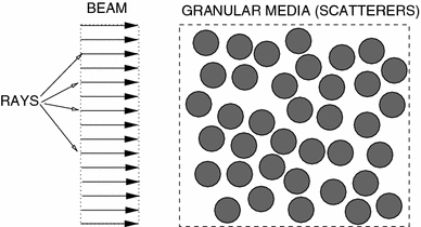
The scattering system considered, comprising a beam, comprising multiple rays, incident on a collection of randomly distributed scatterers
All electromagnetic radiation travels at the speed of light in a vacuum, \(c\approx 3 \times 10^8\) m/s. A more precise value, given by the National Bureau of Standards, is \(c\approx 2.997924562 \times 10^8 \pm 1.1\) m/s. For visible light, the wavelength is between \(3.8 \times 10^{-7}\le \lambda \le 7.2 \times 10^{-7}\) m.
As \(\hat{n}\rightarrow \infty ,\) the object becomes essentially “mirror-like.”
Fig. 3 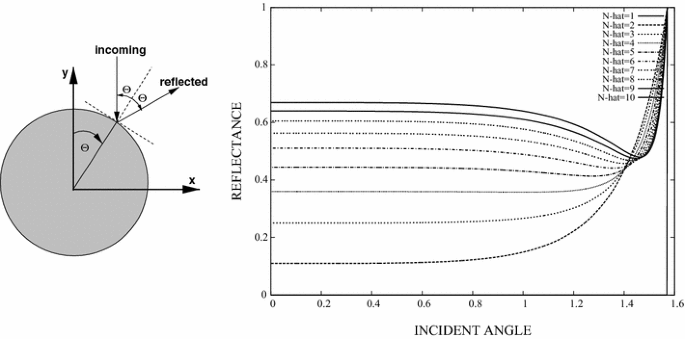
Left a single scatterer. Right the reflectance (R) as a function of incident angle
For example, if one were to arrange the particles in a regular periodic manner, then at the length scale ratio of \(\mathcal{L}=0.25\) the distance between the centers of the particle become four particle radii. In theoretical works, it is often stated that the critical separation distance between particles is approximately three radii to be sufficient to treat the particles as independent scatters, and simply to sum the effects of the individual scatterers to compute the overall response of the aggregate.
Because of the normalized structure of the \(\mathcal{M}\)-metric, it is insensitive to the initial magnitude of \(I_\mathrm{o}.\)
Usually, LIDAR uses high-frequency ultraviolet, visible and near infrared light.
Generally, LIDAR bears some similarity with particle image velocimetry technologies.
Throughout the analysis we assume that \(\hat{n}\ge 1.\)
The limiting case \(\frac{\sin \theta ^*_\mathrm{i}}{\hat{n}}=1,\) is the critical angle (\(\theta ^*_\mathrm{i}\)) case.


References
Avci B, Wriggers P (2012) A DEM-FEM coupling approach for the direct numerical simulation of 3D particulate flows. J Appl Mech 79(1–7):010901
Bohren C, Huffman D (1998) Absorption and scattering of light by small particles. Wiley Science Paperback Series, Weinheim
Bolintineanu DS, Grest GS, Lechman JB, Pierce F, Plimpton SJ, Schunk PR (2014) Particle dynamics modeling methods for colloid suspensions. Comput Part Mech 1(3):321–356
Cante J, Davalos C, Hernandez JA, Oliver J, Jonsen P, Gustafsson G, Haggblad HA (2014) PFEM-based modeling of industrial granular flows. Comput Part Mech 1(1):47–70
Carbonell JM, Onate E, Suarez B (2010) Modeling of ground excavation with the particle finite element method. J Eng Mech ASCE 136:455–463
Cerveny V, Molotkov IA, Psencik I (1977) Ray methods in seismology. Univerzita Karlova, Praha
Cracknell AP, Hayes L (2007) Introduction to remote sensing, vol 2. Taylor and Francis, London. ISBN 0-8493-9255-1. OCLC 70765252
Donev A, Cisse I, Sachs D, Variano EA, Stillinger F, Connelly R, Torquato S, Chaikin P (2004a) Improving the density of jammed disordered packings using ellipsoids. Science 303:990–993
Donev A, Stillinger FH, Chaikin PM, Torquato S (2004b) Unusually dense crystal ellipsoid packings. Phys Rev Lett 92:255506
Donev A, Torquato S, Stillinger F (2005a) Neighbor list collision-driven molecular dynamics simulation for nonspherical hard particles—I. Algorithmic details. J Comput Phys 202:737
Donev A, Torquato S, Stillinger F (2005b) Neighbor list collision-driven molecular dynamics simulation for nonspherical hard particles—II. Application to ellipses and ellipsoids. J Comput Phys 202:765
Donev A, Torquato S, Stillinger FH (2005c) Pair correlation function characteristics of nearly jammed disordered and ordered hard-sphere packings. Phys Rev E 71:011105
Duran J (1997) Sands, powders and grains. An introduction to the physics of Granular Matter. Springer, New York
Elmore WC, Heald MA (1985) Physics of waves. Dover Publications, New York (re-issue)
Goyer GG, Watson R (1963) The laser and its application to meteorology. Bull Am Meteorol Soc 44(9):564–575 [568]
Gross H (2005) In: Gross H (ed) Handbook of optical systems. Fundamental of technical optics. Wiley-VCH, Weinheim
Kansaal A, Torquato S, Stillinger F (2002) Diversity of order and densities in jammed hard-particle packings. Phys Rev E 66:041109
Jackson JD (1998) Classical electrodynamics, 3rd edn. Wiley, New York
Labra C, Onate E (2009) High-density sphere packing for discrete element method simulations. Commun Numer Methods Eng 25(7):837–849
Medina A, Gaya F, Pozo F (2006) Compact laser radar and three-dimensional camera. J Opt Soc Am A 23:800–805
Leonardi A, Wittel FK, Mendoza M, Herrmann HJ (2014) Coupled DEM-LBM method for the free-surface simulation of heterogeneous suspensions. Comput Part Mech 1(1):3–13
Onate E, Idelsohn SR, Celigueta MA, Rossi R (2008) Advances in the particle finite element method for the analysis of fluid–multibody interaction and bed erosion in free surface flows. Comput Methods Appl Mech Eng 197(19–20):1777–1800
Onate E, Celigueta MA, Idelsohn SR, Salazar F, Surez B (2011) Possibilities of the particle finite element method for fluid–soil–structure interaction problems. Comput Mech 48:307–318
Onate E, Celigueta MA, Latorre S, Casas G, Rossi R, Rojek J (2014) Lagrangian analysis of multiscale particulate flows with the particle finite element method. Comput Part Mech 1(1):85–102
Pöschel T, Schwager T (2004) Computational granular dynamics. Springer, New York
Ring J (1963) The laser in astronomy. N Sci June:672–673
Rojek J (2014) Discrete element thermomechanical modelling of rock cutting with valuation of tool wear. Comput Part Mech 1(1):71–84
Rojek J, Labra C, Su O, Onate E (2012) Comparative study of different discrete element models and evaluation of equivalent micromechanical parameters, Int J Solids Struct 49:1497–1517. doi:10.1016/j.ijsolstr.2012.02.032
Torquato S (2002) Random heterogeneous materials: microstructure & macroscopic properties. Springer, New York
Trickey E, Church P, Cao X (2013) Characterization of the OPAL obscurant penetrating LiDAR in various degraded visual environments. In: Proceedings of SPIE 8737, degraded visual environments: enhanced, synthetic, and external vision solutions 2013, 87370E, 16 May 2013. doi:10.1117/12.2015259
van de Hulst HC (1981) Light scattering by small particles. Dover Publications, New York (re-issue)
Widom B (1966) Random sequential addition of hard spheres to a volume. J Chem Phys 44:3888–3894
Zohdi TI (2004) A computational framework for agglomeration in thermo-chemically reacting granular flows. Proc R Soc 460(2052):3421–3445
Zohdi TI (2005) Charge-induced clustering in multifield particulate flow. Int J Numer Methods Eng 62(7):870–898
Zohdi TI (2006a) On the optical thickness of disordered particulate media. Mech Mater 38:969–981
Zohdi TI (2006b) Computation of the coupled thermo-optical scattering properties of random particulate systems. Comput Methods Appl Mech Eng 195:5813–5830
Zohdi TI (2007) Computation of strongly coupled multifield interaction in particle-fluid systems. Comput Methods Appl Mech Eng 196:3927–3950
Zohdi TI (2010) On the dynamics of charged electromagnetic particulate jets. Arch Comput Methods Eng 17(2):109–135
Zohdi TI (2012a) Electromagnetic properties of multiphase dielectrics. A primer on modeling, theory and computation. Springer, New York
Zohdi TI (2012b) Dynamics of charged particulate systems. Modeling, theory and computation. Springer, New York
Zohdi TI (2013a) Numerical simulation of charged particulate cluster-droplet impact on electrified surfaces. J Comput Phys 233:509–526
Zohdi TI (2013b) Rapid simulation of laser processing of discrete particulate materials. Arch Comput Methods Eng 20:309–325
Zohdi T (2014) Embedded electromagnetically sensitive particle motion in functionalized fluids. Comput Part Mech 1(1):27–45
Zohdi TI (2015) A computational modelling framework for high-frequency particulate obscurant cloud performance. Int J Eng Sci 89:75–85
Zohdi TI, Kuypers FA (2006c) Modeling and rapid simulation of multiple red blood cell light scattering. Proc R Soc Interface 3(11):823–831
Author information
Authors and Affiliations
Corresponding author
Ethics declarations
Conflicts of interest
The author declares that he has no conflicts of interest for this research.
Appendix: Generalized Fresnel relations
Appendix: Generalized Fresnel relations
Following a generalization of the Fresnel relations for unequal magnetic permeabilities in Zohdi [35, 36] and Zohdi and Kuypers [45], we consider a plane harmonic wave incident upon a plane boundary separating two different optical materials, which produces a reflected wave and a transmitted (refracted) wave (Fig. 2). Two cases for the electric field vector are considered: (1) electric field vectors that are parallel (||) to the plane of incidence and (2) electric field vectors that are perpendicular (\(\perp \)) to the plane of incidence. In either case, the tangential components of the electric and magnetic fields are required to be continuous across the interface. Consider case (1). We have the following general vectorial representations
where \(\varvec{e}_1\) and \(\varvec{e}_2\) are orthogonal to the propagation direction \(\varvec{k}.\) By employing the law of refraction (\(n_\mathrm{i}\sin \theta _\mathrm{i}=n_\mathrm{t}\sin \theta _\mathrm{t}\)), we obtain the following conditions relating the incident, reflected and transmitted components of the electric field quantities
Since, for plane harmonic waves, the magnetic and electric field amplitudes are related by \(H=\frac{E}{v\mu },\) we have
where \(\hat{\mu }\mathop {=}\limits ^\mathrm{def}\frac{\mu _\mathrm{t}}{\mu _\mathrm{i}},\,\hat{n}\mathop {=}\limits ^\mathrm{def}\frac{n_\mathrm{t}}{n_\mathrm{i}}\) and where \(v_\mathrm{i},\,v_\mathrm{r}\) and \(v_\mathrm{t}\) are the values of the velocity in the incident, reflected and transmitted directions.Footnote 8 By again employing the law of refraction, we obtain the Fresnel reflection and transmission coefficients, generalized for the case of unequal magnetic permeabilities
Following the same procedure for case (2), where the components of \(\varvec{E}\) are perpendicular to the plane of incidence, we have
Our primary interest is in the reflections. We define the reflectances as
Particularly convenient forms for the reflections are
Thus, the total energy reflected can be characterized by
If the resultant plane of oscillation of the (polarized) wave makes an angle of \(\gamma _\mathrm{i}\) with the plane of incidence, then
and it follows from the previous definition of I that
Substituting these expression back into the expressions for the reflectances yields
For natural or unpolarized radiation, the angle \(\gamma _\mathrm{i}\) varies rapidly in a random manner, as does the field amplitude. Thus, since
and therefore for natural radiation
and therefore
Thus, the total reflectance becomes
where \(0\le R\le 1.\) For the cases where \(\sin \theta _\mathrm{t}=\frac{\sin \theta _\mathrm{i}}{\hat{n}}>1,\) one may rewrite reflection relations as
where, \(j=\sqrt{-1},\) and in this complex caseFootnote 9
where \(\bar{r}_{||}\) and \(\bar{r}_{\perp }\) are complex conjugates. Thus, for angles above the critical angle \(\theta ^*_\mathrm{i},\) all of the energy is reflected. Notice that as \(\hat{n}\rightarrow 1\) we have complete absorption, while as \(\hat{n}\rightarrow \infty \) we have complete reflection. The total amount of absorbed power by the particles is \((1-R)I_\mathrm{i}.\) Thermal (infrared) coupling effects, which are outside of the scope of this paper, have been accounted for in Zohdi [35, 36] and Zohdi and Kuypers [45].
In order to understand the dependency of the results on \(\hat{n},\) recall the fundamental relation for reflectance
whose variation as a function of the angle \(\theta _\mathrm{i}\) is depicted in Fig. 3. For all but \(\hat{n}=2,\) is there discernible nonmonotone behavior. The nonmonotone behavior is slight for \(\hat{n}=4,\) but nonetheless present. Clearly, as \(\hat{n}\rightarrow \infty ,\,R\rightarrow 1,\) no matter what the angle of incidence’s value. Also, as \(\hat{n}\rightarrow 1,\) provided that \(\hat{\mu }=1,\,R\rightarrow 0,\) i.e., all incident energy is absorbed. With increasing \(\hat{n},\) the angle for minimum reflectance grows larger.
Rights and permissions
About this article

Cite this article
Zohdi, T.I. On high-frequency radiation scattering sensitivity to surface roughness in particulate media. Comp. Part. Mech. 4, 13–22 (2017). https://doi.org/10.1007/s40571-016-0118-3
Received:
Revised:
Accepted:
Published:
Issue Date:
DOI: https://doi.org/10.1007/s40571-016-0118-3