Power-flow-tracing-based congestion management in hydro-thermal optimal power flow algorithm

Abstract

This paper presents a method for managing congestion constraints in a hydro-thermal optimal power flow solution procedure. The congestion constraint is handled in this paper as an active power generation constraint. To achieve this solution, a power flow tracing technique is used to detect the generators contributing to line congestion to penalize them by reducing their outputs. The congestion is then removed by setting the maximum power of the affected generators to the penalized value. The proposed algorithm is implemented using MATLAB software. Finally, the performance of the proposed algorithm is tested and the results for the 5-bus, 30-bus, and 34-bus Nigerian power networks are presented.

1 Introduction

Congestion arises when a transmission line is operated above its thermal limits. It may occur in power system owing to contingencies that are not anticipated; examples of such contingencies are generation outages, sudden increase in load, transmission line outages, and failure of equipment [1]. Congestion may also be caused through the simultaneous delivery of power from a set of power transactions, thereby exceeding the transmission network limits [2].

Congestion management (CM) refers to the scheduling of available power to avoid or relieve congestion. CM depends on the type of power market. In the regulated power market, where the scheduling of generation is performed following a centralized dispatch, congestions are easier to manage. However, the open-access market is more complex, where the scheduling of generation is not centrally dispatched, but based primarily on the transaction agreed to by market participants. In this situation, the difficulty lies in ensuring the negotiated transactions, particularly under congestion, as CM must be performed in a nondiscriminatory manner [3, 4].

Various approaches to solving the CM problem have been discussed by different authors. In [5], these approaches are categorized into different forms. These categories are technical or cost-free, and financial or non-cost-free. Methods such as the outage of congested lines and use of transmission line compensators are regarded as technical or cost-free approaches, whereas the rescheduling of generation and curtailing of transaction are regarded as financial or non-cost-free approaches [6, 7]. The cost-free measures were coined because of nominal economical consideration as these measures would not involve generation and distribution companies [5]. However, [8] categorized some approaches into short-term and long-term approaches. The short-term transmission CM is based on rules and pricing while the long-term transmission management involves installing new lines, utilizing flexible alternating current transmission systems (FACTS) devices and grid planning to determine the part of a network that should be developed in the future.

The rescheduling of generation and curtailment of transactions as an approach to the solution to CM has received great attention, as different studies have reported various methods in the rescheduling of generation and curtailment of transactions [5, 9]. Congestion pricing is a generation rescheduling method in CM, in which the cost information of the generating companies is either revealed by the generating companies, or it is inferred from the market behavior after which an optimal power flow (OPF) solution procedure (without the consideration of transmission limit) is applied to determine the initial state of the system. If a transmission line congestion is discovered, an OPF analysis (with the consideration of transmission limit) is performed to relieve the system of congestion, and simultaneously determine a congestion price that will be paid by the power producer [10]. Generator sensitivity to the real power flow in a congested line has also been used to reschedule generation to alleviate transmission congestion by proposing a technique for reducing the number of participating generators in a pool at the minimum congestion or rescheduling cost [11,12,13]. In a work that considered a power market where pool and bilateral/multilateral transactions coexist, transaction curtailment strategies were prioritized into the free mode, the pool protection mode, and the contract protection mode [14]. In the free mode, all market participants are expected to compete for usage of congested lines by paying to avoid curtailment. In the pool protection mode, curtailment is performed on bilateral and multilateral transactions first. In the contract protection mode, contract dispatch is prioritized over pool dispatch, i.e., in the case of congestion, the pool demand will have to be curtailed first. In the majority of works where the rescheduling of generation or curtailment of transaction was used as a tool for CM, the primary objective is to minimize the cost of congestion [15]. This minimization was performed using a CM-based OPF.

The usage of transmission line compensators such as FACTS devices have also been considered for CM. Examples of FACTS devices used in alleviating line overloads and increasing transfer capability by controlling power flow are the thyristor-controlled series compensator, static synchronous series compensator, unified power flow controller, and thyristor-controlled phase-angle regulator [5]. However, the effectiveness of these FACTS devices primarily depends on their locations [16].

The identification of generators causing congestion on a transmission line was also adopted in some works as a first step in CM strategy. This was achieved by the power flow tracing technique. This allowed the system operator to penalize only the congestion-contributing generators. In one of these works [17], where generation contribution factor was used as an approach for CM, generator redispatching was performed by decreasing the output of the most congestion-contributing generator and increasing the output of the least congestion-contributing generator to balance the system. This was performed without penalizing the generators between the two extremes of the most and least congestion-contributing generators. In other works [18,19,20], the rescheduling of generation was performed by increasing the output of some congestion-contributing generators and reducing the output of others.

It is important to note that, the extent of contribution of generator to congestion is supposed to dictate the extent of output curtailment by the system operator. However, from the power-flow-tracing-based CM strategies available in literature, it has been discovered as follows:

• 1) Not all the outputs of the congestion-contributing generators are curtailed. Instead, the outputs of some generators are increased. This appears to be discriminatory, especially in a deregulated market where bilateral or multilateral transactions are performed.

• 2) Considering the importance of optimization in the planning and operation of power systems, none of these works considered the power-flow-tracing-based CM in either the OPF or the hydro-thermal optimal power flow (HTOPF) solution technique.

Hence, this work optimally solves the transmission congestion problem of a system with both hydro and thermal generators using the basics of power flow tracing, as opposed to the use of the power flow equation constraint. If congestion occurs, power flow tracing is used to identify the generators contributing to congestion. The congestion-contributing generators at a particular time interval is curtailed and the maximum active output of the affected generators is set to the curtailed value. Hence, the congestion constraint is converted to active power constraint of the affected generator. This renders the proposed solution procedure efficient as the partial differentials of the equations representing the active flow constraints are not considered in the proposed algorithm.

2 HTOPF problem definition

The HTOPF problem is similar to OPF problem, but with an additional constraint representing the water availability of each hydro station. The HTOPF problem can be formulated as follows [21]:

$$ \hbox{min} \, F = \sum\limits_{t = 1}^{T} {\sum\limits_{j = 1}^{{n_{t} }} {(a_{j} + b_{j} P_{jt} + c_{j} P_{jt}^{2} )} } $$

(1)

where F is the total cost of generation for the optimization period; t is the discrete time interval; T is the optimization period under consideration; a_j, b_j, and c_j are the cost coefficients of thermal station j; n_t is the number of thermal generators in the system; and P_jt is the real power output of thermal generator j at time t.

Equation (1) is subjects to the equality constraints as follows.

• 1) Power balance constraints

$$ \left\{ {\begin{array}{*{20}l} {P_{it} + P_{dit} - \, P_{git} = 0} \hfill \\ {Q_{it} + Q_{dit} - \, Q_{git} = 0} \hfill \\ \end{array} } \right. $$

(2)

where t = 1, 2, …, T; P_it and Q_it are the active and reactive power injections, respectively, at bus i during time t, as expressed in (3); P_dit and Q_dit are the active and reactive power demands at bus i during time t, respectively; P_git and Q_git are the scheduled active and reactive power generations of either the thermal station (i.e., P_jt) or hydro station (i.e., P_ht)) at bus i during time t.

$$ \left\{ {\begin{array}{*{20}l} {P_{it} = V_{it} \sum\limits_{k = 1}^{{n_{b} }} {V_{kt} Y_{ik} \cos (\delta_{kt} - \delta_{it} + \theta_{ik} ) \, } } \hfill \\ {Q_{it} = - V_{it} \sum\limits_{k = 1}^{{n_{b} }} {V_{kt} Y_{ik} \sin (\delta_{kt} - \delta_{it} + \theta_{ik} ) \, } } \hfill \\ \end{array} } \right. $$

(3)

where V_it and V_kt are the voltage magnitudes at buses i and k during time t, respectively; n_b is the number of buses in the system; δ_it and δ_kt are the voltage phase angles at buses i and k during time t, respectively; Y_ik and θ_ik are the magnitude and angle of the admittance of the line connecting buses i and k.

• 2) Available water energy constraints

$$ q_{h} - \sum\limits_{t = 1}^{T} {\left( {\alpha_{h} + \beta_{h} P_{ht} + \gamma_{h} P_{ht}^{2} } \right)} = 0\quad h = 1,2, \ldots ,n_{h} $$

(4)

where q_h is the pre-specified amount of water required for generation at hydro station h during the optimization period; α_h, β_h, and γ_h are the discharge coefficients of hydro station h; P_ht is the real output power of the hydro station h at time t; n_h is the number of hydro generators in the system.

• 3) Inequality constraints

$$ \left\{ {\begin{array}{*{20}l} {P_{git}^{\hbox{min} } \le P_{git} \le P_{git}^{\hbox{max} } } \hfill \\ {Q_{git}^{\hbox{min} } \le Q_{git} \le Q_{git}^{\hbox{max} } } \hfill \\ {V_{it}^{\hbox{min} } \le V_{it} \le V_{it}^{\hbox{max} } } \hfill \\ {V_{kt}^{\hbox{min} } \le V_{kt} \le V_{kt}^{\hbox{max} } } \hfill \\ \end{array} } \right. $$

(5)

where superscripts max and min represent the maximum and minimum limits on the variables, respectively.

3 Modified HTOPF solution technique using Newton’s approach

In [22], a modified Newton-based solution technique was developed to solve the problem represented by (1), (2), (4), and (5). The first approach to the development of the solution technique is by augmenting the power balance constraints of (2) with the objective function of (1). The resulting augmented Lagrangian function is shown in (6). It should be noted that, the second term of (6) contains the discharge characteristics of the hydro plants.

$$ \begin{aligned} L_{t} (\varvec{z},\varvec{\lambda},\varvec{\upsilon}) & = \sum\limits_{j = 1}^{{n_{t} }} {(a_{j} + b_{j} P_{jt} + c_{j} P_{jt}^{2} )} \\ & \quad + \sum\limits_{h = 1}^{{n_{h} }} {\upsilon_{h} (\alpha_{h} + \beta_{h} P_{ht} + \gamma_{h} P_{ht}^{2} )} \\ & \quad + \sum\limits_{i = 1}^{{n_{b} }} {\lambda_{pit} (P_{it} + \, P_{dit} - P_{git} )} \\ & \quad + \sum\limits_{i = 1}^{{n_{b} }} {\lambda_{qit} (Q_{it} + \, Q_{dit} - Q_{git} )} \\ \end{aligned} $$

(6)

where $\varvec{\upsilon}= \left( {\upsilon_{h} } \right)$; t = 1, 2, …, T; $\varvec{z} = \left[ {\delta_{it} ,\delta_{kt} ,V_{kt} ,V_{it} ,P_{git} } \right]$; $\varvec{\lambda}= \left[ {\lambda_{pit} ,\lambda_{qit} } \right]$; λ_pit is the Lagrange multiplier relating to the active power balance equation at bus i during time interval t; λ_qit is the Lagrange multiplier relating to the reactive power balance equation at bus i during time interval t; υ_h is the water worth or water conversion factor for an optimization period.

It is important to note that (6) does not cater for the water energy constraint of (4). This constraint is however considered after minimizing all the T Lagrangian sub-equations. Further, CM constraints are not considered in the work.

The optimal solution to (6) is achieved by satisfying the Karush–Kuhn–Tucker (KKT) condition for optimality given in (7) and (8) [21, 23].

$$ \frac{{\partial L_{t} }}{{\partial \varvec{z}}} = \nabla_{\varvec{z}} L_{t} = \left[ {\begin{array}{*{20}c} {\frac{{\partial L_{t} }}{{\partial \delta_{it} }}} & {\frac{{\partial L_{t} }}{{\partial \delta_{kt} }}} & {\frac{{\partial L_{t} }}{{\partial V_{it} }}} & {\frac{{\partial L_{t} }}{{\partial V_{kt} }}} & {\frac{{\partial L_{t} }}{{\partial P_{git} }}} \\ \end{array} } \right]^{\text{T}} = {\mathbf{0}} $$

(7)

$$ \frac{{\partial L_{t} }}{{\partial\varvec{\lambda}}} = \nabla_{\varvec{\lambda}} L_{t} = \left[ {\begin{array}{*{20}c} {\frac{{\partial L_{t} }}{{\partial \lambda_{pit} }}} & {\frac{{\partial L_{t} }}{{\partial \lambda_{qit} }}} \\ \end{array} } \right]^{\text{T}} = {\mathbf{0}} $$

(8)

The KKT optimality condition yielded a set of nonlinear equations that are solved using the Newton–Raphson method. This method requires linearizing these equations and the resulting equation is shown in (9).

$$ \, \left[ {\begin{array}{*{20}c} {\frac{{\partial^{2} L_{t} }}{{\partial \varvec{z}^{ 2} }}} & {\frac{{\partial^{2} L_{t} }}{{\partial \varvec{z}\partial\varvec{\lambda}}}} \\ {\frac{{\partial^{2} L_{t} }}{{\partial\varvec{\lambda}\partial \varvec{z}}}} & {\frac{{\partial^{2} L_{t} }}{{\partial\varvec{\lambda}^{ 2} }}} \\ \end{array} } \right] \, \left[ {\begin{array}{*{20}c} {\Delta \varvec{z}} \\ {\Delta\varvec{\lambda}} \\ \end{array} } \right] = \, \left[ {\begin{array}{*{20}c} {\nabla_{\varvec{z}} L_{t} } \\ {\nabla_{\varvec{\lambda}} L_{t} } \\ \end{array} } \right] \, $$

(9)

where $\left[ {\nabla_{\varvec{z}} L_{t} ,\nabla_{\varvec{\lambda}} L_{t} } \right]^{\text{T}}$ is the gradient vector; ∆z and ∆λ are the increments or decrements on the control and state variables, respectively; $\left[ {\begin{array}{*{20}c} {\frac{{\partial^{2} L_{t} }}{{\partial \varvec{z}^{ 2} }}} & {\frac{{\partial^{2} L_{t} }}{{\partial \varvec{z}\partial\varvec{\lambda}}}} \\ {\frac{{\partial^{2} L_{t} }}{{\partial\varvec{\lambda}\partial \varvec{z}}}} & {\frac{{\partial^{2} L_{t} }}{{\partial\varvec{\lambda}^{ 2} }}} \\ \end{array} } \right]$ is the Hessian matrix.

Equation (9) is solved iteratively; for every iteration, the variables (z and λ) are updated using the equation below:

$$ \left\{ {\begin{array}{*{20}l} {\varvec{z}_{{{new} }} = \varvec{z}_{{{old} }} - \Delta \varvec{z}} \hfill \\ {\varvec{\lambda}_{{{new} }} =\varvec{\lambda}_{{{old} }} - \Delta\varvec{\lambda}} \hfill \\ \end{array} } \right. $$

(10)

A solution is reached when the gradient vectors of (7) and (8) are within the tolerance margin. If any of the variables listed in (5) is outside the allowable limits, the inequality constraint is enforced according to the criteria given in [24].

It should be noted that (6) requires having T Lagrangian sub-equations. Each equation is minimized separately and the results for all the equations are used to update the water worth value. This procedure continues until the water worth value tracked the available water. The water worth value is updated using (11).

$$ \Delta \upsilon_{h}^{(m)} = - \frac{{\Delta q_{h}^{(m)} }}{{A^{(m)} }} $$

(11)

where $A = \sum\nolimits_{i = 1}^{t} {\lambda_{pit}^{2} /(2\gamma_{h} \upsilon_{h}^{3} )}$.

Therefore, at iteration m + 1, the water worth value is adjusted using the equation below:

$$ \upsilon_{h}^{(m + 1)} = \upsilon_{h}^{(m)} + \Delta \upsilon_{h}^{(m)} $$

(12)

The flow chart used to implement the procedure explained above is shown in Fig. 1. The summary of the flow chart is as presented below:

Fig. 1

Flow chart for solving HTOPF problem

• 1) The iteration loops are represented by the arrow head arc with a loop number written inside it.

• 2) The first step is the variable initialization.

• 3) Iteration loop 1 solves (9) and updates the HTOPF variables (except the water worth value) until the gradient vector mismatch is less than or equal to the tolerable limit of 10⁻⁴.

• 4) Iteration loop 2 ensures that all the HTOPF variables from loop 1 are within bounds, while ensuring that the gradient vector mismatch is less than or equal to the tolerable limit of 10⁻⁴.

• 5) The optimization interval loop 3 allows for solving for the next optimization interval t.

• 6) At a given interval t = T, iteration loop 4 is entered to verify if the water availability mismatch |q_h| is less than or equal to the tolerable limit; if it is not, an update of the water worth value is required.

This procedure continues until the water energy constraint is satisfied. Figure 1 was implemented using the MATLAB software. The software was used to solve various power systems’ problem. The results obtained proved the effectiveness of the procedure.

4 HTOPF problem with congestion constraints

In the problem defined in Section 3, the congestion constraint is not included. However, the proposed method includes this constraint, as shown below:

$$ P_{ikt} \le P_{ikt}^{{\text{max}}} $$

(13)

where P_ikt is the active power flow on the line connecting buses i and k together at time t, as expressed in (14).

$$ P_{ikt} = - V_{it}^{2} Y_{ik} \cos \theta_{ik} + V_{it} V_{kt} Y_{ik} \cos (\delta_{it} - \delta_{kt} - \theta_{ik} ) $$

(14)

The constraint of (13) is considered by curtailing the generators that contribute to the active flow on the congested line. The contribution of the individual generator is known through power flow tracing. After curtailing the active generation, the maximum active power generation of the affected generators at time t (i.e., $P_{git}^{ \hbox{max} }$) is adjusted such that it is equal to the curtailed value.

Therefore, in this study, the congestion constraints are regarded as active power generation constraints. This is to avoid additional constraint equations in the Lagrangian function.

4.1 Power flow tracing

The power flow tracing concept and its function has been highlighted in the work of [24]. It is important to note that power flow tracing is based on the charges for using the transmission line. However, since this concept can be used to identify the contribution of individual generator to a congested transmission line, the affected generator can be curtailed based on contribution degree to the congestion.

The convenient starting point for power flow tracing methods is dictated by the state of the power system, i.e., the solution of a power flow or OPF or the state estimation computation [25, 26]. To understand the concept of power flow tracing using “source dominion”, a three-bus system with two generators and three transmission lines is used, as shown in Fig. 2. The following procedure is adopted [24].

Fig. 2

Three-bus active power flow diagram

• 1) Calculate the ratio of the active power flow on each line (both sending end and receiving end) to the total active power inflow to the sending bus; represent this as C₁₂, C₁₃, and C_32.

$$ \left\{ {\begin{array}{*{20}l} {C_{12}^{S} = {{P_{12}^{S} } \mathord{\left/ {\vphantom {{P_{12}^{S} } {P_{g1} }}} \right. \kern-0pt} {P_{g1} }}} \hfill \\ {C_{12}^{R} = {{P_{12}^{R} } \mathord{\left/ {\vphantom {{P_{12}^{R} } {P_{g1} }}} \right. \kern-0pt} {P_{g1} }}} \hfill \\ \end{array} } \right. $$

(15)

$$ \left\{ {\begin{array}{*{20}l} {C_{13}^{S} = {{P_{13}^{S} } \mathord{\left/ {\vphantom {{P_{13}^{S} } {P_{g1} }}} \right. \kern-0pt} {P_{g1} }}} \hfill \\ {C_{13}^{R} = {{P_{13}^{R} } \mathord{\left/ {\vphantom {{P_{13}^{R} } {P_{g1} }}} \right. \kern-0pt} {P_{g1} }}} \hfill \\ \end{array} } \right. $$

(16)

$$ \left\{ {\begin{array}{*{20}l} {C_{32}^{S} = {{P_{32}^{S} } \mathord{\left/ {\vphantom {{P_{32}^{S} } {\left( {P_{13}^{R} + P_{g3} } \right)}}} \right. \kern-0pt} {\left( {P_{13}^{R} + P_{g3} } \right)}}} \hfill \\ {C_{32}^{R} = {{P_{32}^{R} } \mathord{\left/ {\vphantom {{P_{32}^{R} } {\left( {P_{13}^{R} + P_{g3} } \right)}}} \right. \kern-0pt} {\left( {P_{13}^{R} + P_{g3} } \right)}}} \hfill \\ \end{array} } \right. $$

(17)

where superscripts S and R denote the sending end and receiving end active line flows, respectively; P₁₂, P₁₃, and P₃₂ are the active power flows on lines 1–2, 1–3, and 3–2, respectively; P_g1 and P_g3 are the active power generations at buses 1 and 3, respectively.

• 2) Form the source dominion for P_g1 and P_g3. This requires identifying the flow path of the active power from each generator. The source dominion for P_g1 and P_g3 are shown in Fig. 3a, b, respectively.

  Fig. 3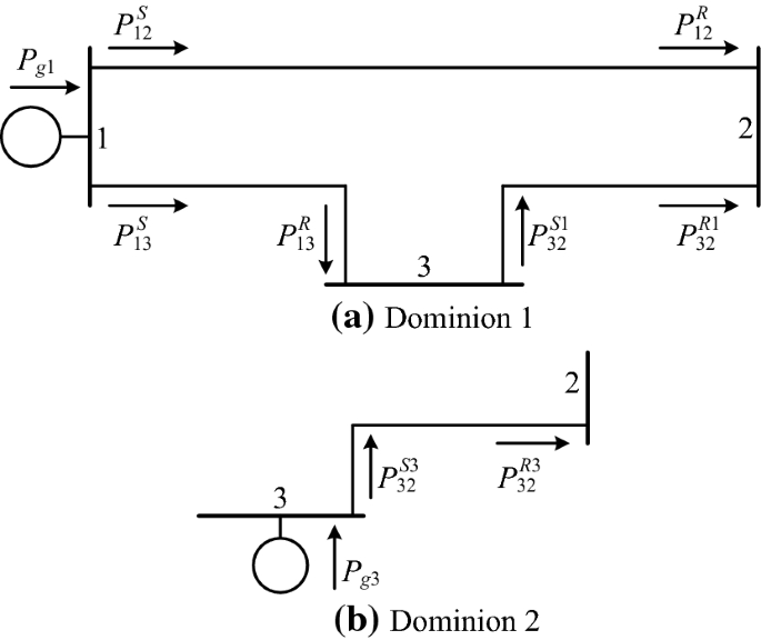

  

  Source dominions

• 3) Calculate the contribution of each dominion to the active line flow. As shown in Fig. 3a, b, lines 1–2 and 1–3 belong to source dominion 1 only while line 3–2 belongs to both sources’ dominion. This implies that only P_g1 contributes to P₁₂ and P₁₃, while P_g1 and P_g3 both contribute to P₃₂.

The contribution of P_g1 to P₃₂ is expressed as follows:

$$ \left\{ {\begin{array}{*{20}l} {P_{32}^{S1} = C_{32}^{S} P_{13}^{R} } \hfill \\ {P_{32}^{R1} = C_{32}^{R} P_{13}^{R} } \hfill \\ \end{array} } \right. $$

(18)

where superscripts S1 and R1 denote the sending end and receiving end active line flows contributed by P_g1, respectively.

Additionally, the contribution of P_g3 to P₃₂ is expressed as follows:

$$ \left\{ {\begin{array}{*{20}l} {P_{32}^{S3} = C_{32}^{S} P_{g3} } \hfill \\ {P_{32}^{R3} = C_{32}^{R} P_{g3} } \hfill \\ \end{array} } \right. $$

(19)

where superscripts S3 and R3 denote the sending end and receiving end active line flows contributed by P_g3, respectively.

It is essential to note that ${P}_{ 1 3}^{R}$ in (18) is the active contribution from source dominion 1, as shown in Fig. 3a.

4.2 Power-flow-tracing-based CM

If transmission line i–j is discovered to be congested, the extent of contribution of the generators in the system is determined using the power flow tracing algorithm. With this information, the output of the affected generator is reduced by a value dictated by the extent of contribution of the generator, as illustrated in (20). The curtailed output of the affected generator i $P_{git,new}^{{}}$ is determined as follows:

$$ P_{git,new}^{{}} = P_{git,old}^{{}} - \frac{{P_{ijt,is}^{{}} }}{{P_{ijt,s}^{{}} }}P_{ijt}^{\hbox{max} } $$

(20)

where $P_{git,old}^{{}}$ is the output of generator at bus i before curtailment at time t; $P_{ijt,is}^{{}}$ is the contribution of generator at bus i to the sending end active flow on line i–j at time t; $P_{ijt}^{{\text{max}}}$ is the maximum active flow on line i–j at time t; $P_{ijt,s}^{{}}$ is the sending end active flow on line i–j.

After the curtailment, the maximum power limit of the affected generator is set to the curtailed power $P_{git,new}^{{}}$ in the developed program discussed in [22]. It should be noted that the curtailment in the system will cause imbalances in power and available water. However, these imbalances are compensated with the developed procedure.

4.3 Flow chart for implementation of a power-flow-tracing-based CM

The flow chart that represents the procedure described in Section 4.2 is shown in Fig. 4. This figure is an adjustment of Fig. 1 to accommodate for the CM procedure. The primary adjustments comprise two steps: ① water worth value initialization to the HTOPF solution value; ② the modification of iteration loops 2 and 3. These modifications are shown in the flow chart as the shapes with colored fill.

Fig. 4

Flow chart for power-flow-tracing-based CM

Unlike Fig. 1, where the water worth value is initialized to the value obtained from the initialization procedure discussed in [22], the water worth value in Fig. 4 is initialized to the value from the HTOPF solution. This is to allow the CM procedure to act on the optimal state of the power system. A close comparison of Figs. 1 and 4 shows that the iteration loops 2 and 3 of Fig. 1 have been modified to accommodate the power-flow-tracing-based CM procedure. The enforcement of congestion limit requires a power flow tracing technique to identify the congestion-contributing generators. A solution is reached when the transmission congestion is removed from all lines while the available water is utilized optimally.

5 Numerical results

The flow chart described in Fig. 4 has been implemented using a MATLAB-based software program. The developed program can accommodate any number of PV and PQ buses. Any of the generator bus in the power network can be made the slack bus.

To evaluate the developed software, it has been used to solve the HTOPF with transmission line congestion problem for the 5-bus, 30-bus, and 34-bus Nigerian power networks. Twenty-four hour load duration intervals have been considered for this work. The test systems and load curve used for this work are similar to those presented in [22]. Two cases are considered in this section: ① case A (base case), HTOPF results as presented in [22]; ② case B, HTOPF results with CM. These cases are compared to study the impact of the proposed CM procedure on the HTOPF solution. It is important to note that the naira to dollar exchange rate used throughout this section is $1 = ₦200. Further, the active power by the thermal generator (TG) at bus J and hydro generator (HG) at bus K are represented as P_gtJ and P_htK, respectively. For example, the TG at bus 1 is represented as P_gt1, and the HG at bus 2 is represented as P_ht2.

5.1 Results for 5-bus Nigerian power network

The proposed algorithm has been tested on this system by setting a real power transmission limit of 55 MW for line 2–3. This caused congestion on the line at hours 7–9 and 18–20, with a maximum base case active power flow violation recorded at hour 7 with a value of 61.1 MW. The active flow during congestion is traceable to the active power of the hydro station at bus 2 (P_ht2), and the congestion is removed optimally. The HTOPF solution is achieved with an absolute maximum water mismatch of 8.01 × 10⁻⁶. Figure 5 shows the active flow on line 2–3 for both cases. The active flow on this line has been curtailed throughout the period. The comparison of results for both cases is shown in Table 1. It is clear from this table that the differences between the HTOPF results for both cases are not highly significant. This is attributed to the computational efficiency of the proposed algorithm. The result with the most significant decrease of 2.77% is the water worth value. The average hydro energy is increased by 0.01%. The curtailment of P_ht2 during the congested hours is responsible for the decrease in the water worth value. The curtailment of P_ht2 has resulted in a slightly better utilization of the available water in case B, as indicated in the average hydro energy. An additional cost of ₦23956.60 is incurred owing to the CM procedure. This cost amounts to a 0.17% increase from the cost obtained for case A.

Fig. 5

Active power flow through line 2–3

Table 1 Comparison of HTOPF results for 5-bus Nigerian power network

The proposed CM procedure adjusted the schedules optimally, while relieving the system of congestion. The readjustment experienced in the system owing to CM is depicted in Fig. 6. This figure shows the percentage difference in the generators’ active power before and after CM. This percentage is determined using the criteria given in (21). From Fig. 6, it is clear that, to maintain power balance during the congested hours, the curtailment of P_ht2 leads to the increase in P_gt1. Further, to maintain water energy balance, P_ht2 has to increase during some uncongested hours. It should be noted that the increase or decrease in the output of one unit at a time instance leads to the respective decrease or increase in the outputs of other units if active power limit enforcement and load shedding do not occur.

$$ C_{\text{P}} = \frac{{P_{gb} - P_{ga} }}{{P_{gb} }} \times 100\% $$

(21)

where C_P denotes percentage difference in the generation; P_gb and P_ga denote the generators’ active power before and after CM.

Fig. 6

Percentage difference in generation in 5-bus system owing to CM

5.2 Results for 30-bus Nigerian power network

The real power transmission limits for lines 1–2 and 6–8 are set at 62 MW and 38 MW, respectively. These caused congestion on both lines. The maximum base case active power flows on these lines are 71 MW and 45.57 MW, respectively, and these values are recorded during hour 7. The active flow during congestion on line 1–2 is traceable to P_gt1 at hours 7–9 and 18–20, while the active flow on line 6–8 is traceable to P_gt8 at hours 5–10 and 17–20. The congestion is removed by curtailing the outputs of the two generators. The active power flows through these lines for both cases are shown in Figs. 7 and 8, respectively. As observed, the flows through these lines are within the limit. The solution after removing congestion is obtained with the maximum absolute water mismatch of 5.55 × 10⁻⁶. The comparison of some system parameters for both cases is shown in Table 2. The table indicates that the most significant difference obtained is the 1.13% increase in the water worth value of both HGs from the base case value. The table also shows a slight decrease in the average hydro plant energy for both plants in case B. The additional cost owing to removing congestion is ₦1016.36, constituting a 0.04% increase. The percentage difference in the system’s active generation is shown in Fig. 9. It is important to note that to maintain power balance, the curtailments of the two generators at the congested periods caused the output of all other generators to increase at these periods. To use the available water optimally, the increase in P_ht5 and P_ht13 at the congested periods necessitated a decrease of these active outputs at the noncongested periods.

Fig. 7

Active power flow through line 1–2

Fig. 8

Active power flow through line 6–8

Table 2 Comparison of HTOPF results for 30-bus Nigerian power network

Fig. 9

Percentage difference in generation in 30-bus Nigerian power network owing to CM

5.3 Results for 34-bus Nigerian power network

The transmission limits for the Benin–Osogbo and Onitsha–Benin transmission lines are set at 340 MW and 230 MW, respectively. The congestion on both lines is noticed at hours 4, and 22–24. The base case maximum active power flows of the two lines are 353.1 MW and 239.2 MW, respectively. The congestion is removed by curtailing only the congestion-contributing generators. The Delta, Sapele, Geregu, Okpai, and Asco generating stations (GSs) contributed to the active flow on the Osogbo–Benin line during congestion, with Geregu being the GS that contributed the most. The Okpai GS is the only station that contributes to the active flow on the Onitsha–Benin line during congestion. Figures 10 and 11 show the active line flow through these lines for the cases considered. It is clear that these lines have been relieved of congestion with the application of the proposed procedure. Alleviating congestion on these lines caused readjustment in the base case active power generation schedule. This readjustment is captured in Fig. 12. To maintain power balance, the curtailments of the affected generators during congestion resulted in an increase in the outputs of other generators. However, to satisfy the water energy constraints, the increase in the outputs of Shiroro, Jebba, and Kainji GSs at the congested hours led to a decrease in their outputs during the uncongested hours. This subsequently resulted in an increase in the thermal stations’ outputs at the uncongested hours. The power limits of Geregu, Okpai, and Asco GSs caused their outputs to not respond at certain uncongested hours.

Fig. 10

Active power flow through Benin–Osogbo line

Fig. 11

Active power flow through Onitsha–Benin line

Fig. 12

Percentage difference in generation in 34-bus Nigerian power network owing to CM

Table 3 presents the HTOPF parameters for the cases considered. The difference in these parameters is insignificant. It should be noted that, the cost of generation is reduced in this system owing to CM. This is as a result of the decrease in the total thermal generation by 16.5 MWh, and an increase in the hydro generation by 6.7 MWh. As the cost of generation depends on the thermal plants, the decrease in total thermal generation leads to the reduced total cost of generation. It should be noted that the Shiroro GS responded the most to the curtailments of the affected generators (see Fig. 12), which are primarily thermal stations. This is attributed to its ability to better maximize its water usage [22]. Therefore, this contributed significantly to further reducing the cost of generation, as shown in Table 3. A decrease in the total transmission loss by 9.7 MWh is also obtained.

Table 3 Comparison of HTOPF results for 34-bus Nigerian power network

5.4 Implication of proposed method on power system market

The proposed methodology is applicable in a completely regulated or partially deregulated market. In any of these two forms of markets, the system operator is involved in the dispatch of generation to ensure system’s security. Figures 6, 9 and 12 show how the adjustments are performed on the outputs of the generators in the system for a 24-hour period. The positive and negative percentage differences indicate a decrease and increase in the generation output, respectively. If a generating company involved in any form of transactions over a 24-hour period has a generator (thermal or hydro) whose output is curtailed at a particular hour owing to congestion, the output of the same generating company is increased at some other hour. So far, no MW-limit is imposed on the generation. This enables the generating company to generate more revenue to mitigate the effect of the earlier curtailments. The proposed methodology ensures that congestion is eliminated such that the available water in a hydro plant is utilized completely.

6 Conclusion

A power-flow-tracing-based CM was proposed to curtail only the congestion-contributing generators at the congested intervals to alleviate congestion and utilize the available water optimally. The MATLAB program was developed to implement the proposed solution procedure. The developed software has been tested on the 5-bus, 30-bus, and 34-bus Nigerian power networks to evaluate its performance.

From the numerical simulations performed, the conclusions are as follows:

• 1) The proposed algorithm has shown that CM in a hydro-thermal system may not lead to an increase in the cost of generation.

• 2) Curtailing the output of a HG during the congested period caused a reduction in water worth value from its base case value, while increasing the output results in the reverse.

• 3) CM is expected to exhibit a deviation in its power system parameters from its typical operating values. However, the proposed algorithm could readjust the generation schedule optimally, such that the differences in the HTOPF parameters for both cases considered are not significant.

• 4) The insignificant differences in values between cases A and B are an indication of the efficiency of the proposed algorithm in removing transmission constraints.

The proposed algorithm allowed the system operator to redispatch, such that an efficient allocation of generation could be implemented when congestion occurs. This allocation of generation is void of discrimination.

Further work may include CM in a power network with thermal, hydro, solar, and wind energy sources.

References

Balaraman S, Kamaraj N (2011) Transmission congestion management using particle swarm optimization. J Electr Syst 7:54–70
Singh H, Hao S, Papalexopoulos A (1998) Transmission congestion management in competitive electricity markets. IEEE Trans Power Syst 13(2):672–680
Srivastava SC, Kumar P (2000) Optimal power dispatch in deregulated market considering congestion management. In: Proceedings of international conference on electric utility deregulation and restructuring and power technologies, London, UK, 4–7 April 2000, pp 53–59
Grgiĉ D, Gubina F (2001) Implementation of the congestion management scheme in unbundled Slovenian power system. In: Proceedings of the IEEE Porto power tech, Porto, Portugal, 10–13 September 2001, 4 pp
Pillay A, Karthikeyan SP, Kothari DP (2015) Congestion management in power systems – a review. Electr Power Energy Syst 70:83–90
Nayak AS, Pai MA (2002) Congestion management in restructured power systems using an optimal power flow framework. Dissertation, University of Illinois
Verma YP, Sharma AK (2015) Congestion management solution under secure bilateral transactions in hybrid electricity market for hydro-thermal combination. Electr Power Energy Syst 64:398–407
Karatekin CZ, Ucak C (2008) Sensitivity analysis based on transmission line susceptances for congestion management. Electr Power Syst Res 78(9):1485–1493
Singla A, Singh K, Yadav VK (2014) Transmission congestion management in deregulated environment: a bibliographical survey. In: Proceedings of the IEEE international conference on recent advances and innovations in engineering (ICRAIE-2014), Jaipur, Indian, 9–11 May 2014, 7 pp
Glavitsch H, Alvarado F (1998) Management of multiple congested conditions in unbundled operation of a power system. IEEE Trans Power Syst 13(3):1013–1019
Dutta S, Singh SP (2008) Optimal rescheduling of generators for congestion management based on particle swarm optimization. IEEE Trans Power Syst 23(4):1560–1569
Kumar A, Kumar V, Chanana S (2009) Generators and loads contribution factors based congestion management in electricity markets. Int J Recent Trends Eng 2:13–16
Boonyaritdachochai P, Boonchuay C, Ongsakul W (2010) Optimal congestion management in an electricity market using particle swarm optimization with time-varying acceleration coefficients. Comput Math Appl 60(4):1068–1077
Fang RS, David AK (1999) Transmission congestion management in an electricity market. IEEE Trans Power Syst 14(3):877–883
Singh K, Padhy NP, Sharma J (2011) Congestion management considering hydro-thermal combined operation in a pool based electricity market. Electr Power Energy Syst 33(8):1513–1519
Yousefi A, Nguyen TT, Zareipour H et al (2012) Congestion management using demand response and FACTS devices. Electr Power Energy Syst 37(1):78–85
Song H, Kezunovic M (2004) A comprehensive contribution factor method for congestion management. In: Proceedings of IEEE PES power systems conference and exposition, New York, USA, 10–13 October 2004, pp 977–981
Yang J, Anderson MA (1999) Tracing the flow of power in transmission networks for use-of-transmission-system charges and congestion management. In: Proceedings of IEEE power engineering society winter meeting, New York, USA, 31 January–4 February 1999, pp 399–405
Rajathy R, Kumar H (2012) Power flow tracing based congestion management using differential evolution in deregulated electricity market. Int J Electr Eng Inform 4:371–392
Basha AAJ, Anitha M (2016) Power flow tracing based congestion management using firefly algorithm in deregulated electricity market. Int J Eng Res Dev 12(5):38–48
El-Hawary ME, Tsang DH (1986) The hydro-thermal optimal load flow: a practical formulation and solution techniques using Newton’s approach. IEEE Trans Power Syst 1(3):157–167
Lawal MO (2016) Hydro-thermal optimal power flow analysis in a deregulated market environment. Dissertation, Obafemi Awolowo University
Sun DI, Ashley B, Brewer B et al (1984) Optimal power flow by Newton approach. IEEE Trans Power Appar Syst 103(10):2864–2880
Acha E, Fuerte-Esquivel CR, Ambriz-Perez H et al (2004) FACTS modeling and simulation in power networks. Wiley, London
Kirschen D, Allan R, Strbac G (1997) Contributions of individual generators to loads and flows. IEEE Trans Power Syst 12(1):52–60
Kirschen D, Strbac G (1999) Tracing active and reactive power between generators and loads using real and imaginary currents. IEEE Trans Power Syst 14(4):1312–1319
Author information
Authors and Affiliations
Corresponding author
Additional information
CrossCheck date: 18 October 2018
Rights and permissions
Open Access This article is distributed under the terms of the Creative Commons Attribution 4.0 International License (http://creativecommons.org/licenses/by/4.0/), which permits unrestricted use, distribution, and reproduction in any medium, provided you give appropriate credit to the original author(s) and the source, provide a link to the Creative Commons license, and indicate if changes were made.
About this article
Cite this article
LAWAL, M.O., KOMOLAFE, O. & AJEWOLE, T.O. Power-flow-tracing-based congestion management in hydro-thermal optimal power flow algorithm. J. Mod. Power Syst. Clean Energy 7, 538–548 (2019). https://doi.org/10.1007/s40565-018-0490-5
Received:
Accepted:
Published:
Issue Date:
DOI: https://doi.org/10.1007/s40565-018-0490-5