
Abstract
The paper presents simulations of mechanical properties of compressed expanded graphite. To model the stress and strain states of compressed expanded graphite, a hyperelastic material model formulated by the Blatz–Ko was adapted. The idea of using this model resulted from the assumptions that compressed expanded graphite exhibits similar mechanical properties to polyurethane foam with high density. The material constant of the Blatz–Ko model was determined by numerical calculations where deformation energy equation was parameterized with the shear modulus. Such material model used in a compressed expanded graphite simulation was experimentally validated. Subsequently, the Blatz–Ko model was used in a numerical simulation of the graphite-metallic structure in the form of a spiral wound gasket which is composed of metallic and elastic tapes. This structure was subjected to an optimization process which included the reduction of stress in the elastic graphite tape obtaining the appropriate axial stiffness of the gasket. In the final stage, the optimal design of the gasket was experimentally tested. The experimental results were compared with the data obtained numerically, which allowed to verify the adapted material model and boundary conditions of the numerical gasket model.
1 Introduction
Expanded graphite (EG) is a material produced from natural graphite (NG) in a chemical and thermal process called exfoliation [1]. Due to this process, its volume increases even up to 400 times. EG is widely used as an addition to various types of nano-composites [2,3,4,5,6,7]. It inherited lots of favorable features of NG, i.e., it exhibits high chemical and thermal resistance [8, 9]. Paper [10] presents an innovative investigation method and test results concerning elastic properties of EG. As it was found, EG’s elastic modulus strongly depends on the direction of measurement. For instance, the value in-plane of compression is bigger than values measured out-of-plane at the same density level. The mechanical, electrical and chemical properties of EG were presented in [11]. In accordance with an experimental test, it was proved that all properties of EG can be approximated by means of the power law. The most popular form of EG used in industry is compressed expanded graphite (CEG). It characterizes with high mechanical strength, especially at a compression load [12]. Due to these properties, CEG can be utilized in various industrial applications [13]. Good elasticity and low permeability of fluids caused that CEG is widely used in sealing technology [14]. In industry CEG is utilized as thin, laminated foil with bulk density ranging from 0.5 to 1.5 g/cm3. Its drawbacks are big losses of mass in contact with oxygen, especially at an elevated temperature. The degree of CEG oxidation depends on its purity, particularly on sulfur contents, which is usually in a range from 300 to 1000 ppm. Mechanical strength, in case of a tensile load, is low and ranges from 2 to 6 MPa [12]. In case of a compression load, the destructive contact pressure of CEG’s laminated foil is (depending on foil thickness) from 180 MPa (at thickness 1 mm) to 300 MPa (at thickness 0.35 mm). In sealing technology, CEG has found an application as filler used in, so called, semi-metal gaskets of the flange-bolted joints. The most popular form is the spiral wound gasket (SWG). More details concerning this structure were presented in chapter 5; however, it is worth to mention its main features. The advantage of SWG is a very small leakage level at relatively low bolts’ load [15, 16]. The quality of a gasket strongly depends on CEG’s properties, predominantly on its packing density in the spiral structure [17, 18]. The main disadvantage is the limited compressive strength, since at an excessive load the internal windings of the spiral could be buckled [19,20,21,22,23]. Another important issue is the gasket’s stiffness. In line with the standard ASME 16.20 2017, stiffness should be properly designed depending on the size of the pipe’s nominal diameter and the sealing pressure. In order to increase the stiffness, the spiral is wound tighter or embedded in metal rings: internal and/or external ones. The use of these rings and their influence on the gasket’s stiffness were presented in [15]. Another solution that enhances stiffness of the gasket is proper shaping of the tape’s cross section [24]. The most common tool accelerating the process of the structure optimization is the finite element method (FEM). In case of gaskets’ modeling, this method is also used as presented in papers [25, 26]. The most challenging issue in the numerical modeling of CEG is the proper selection of the material model mapping its elastic behavior. Based on results presented in [27], it was proved that treating CEG as an isotropic, linear material causes a big discrepancy between numerical results and experimental ones. In this paper, the new approach was proposed to reflect elastic properties of CEG by means of a nonlinear material model. Based on the experimental compression test of CEG, it was found that the characteristic describing the relationship between stress–strain could be, with high accuracy, modeled with a nonlinear compressible hyperelastic Blatz–Ko model. In the further step, this model was used in a numerical simulation of the graphite-metallic structure in the form of SWG. This structure was subjected to the optimization process which included stress reduction in the elastic graphite tape and obtaining the appropriate axial stiffness of the gasket.
2 CEG elastic properties
The main difference between EG and NG is their internal structure which is presented in Fig. 1. The structure of EG is more porous due to the exfoliation process. When it comes to mechanical properties, NG is an isotropic material and non-compressible, whereas EG exhibits a nonlinear effect with high compressibility and plasticity levels. During the compression of EG, its bulk density increases and as a result the elastic modulus can change even up to several orders of magnitude (Fig. 2).

The internal structure of graphite; a natural graphite, b, c expanded graphite [5]

Elasticity modulus versus bulk density of (EG) [7]
The approximate value of CEG elastic modulus at the compression load can be mapped with a great accuracy by means of the empirical Eq. (1) [10].
where \(E_{0}\) is the elastic modulus at 0% porosity, \(P\) is the porosity level, \(a,n\) are the material constants.
High dependence of CEG’s elastic modulus on the compression level causes that the use of a constant value to model the stress and strain of the structures made of CEG can lead to large discrepancies between the model and real behavior of the material under load [27]. Nonlinear dependence between the stress and strain of CEG under compression proves that the elastic modulus is strongly progressive. Similar properties exhibit foamed elastomeric materials. The most similar mechanical properties to CEG have materials made of polyurethane foam (PUF) (especially rigid PUF with high bulk density, Fig. 3). Similarities can be found in mechanical properties (Table 1) and in the same course of the curve describing the relationship between stress and strain at the compression load [29,30,31,32,33,34].

Compressive characteristics of CEG foil and polyurethane foam
3 Constitutive material model
Due to the fact that CEG exhibits similar mechanical properties to PUF, its stress–strain relationship could be treated as a compressible elastomeric material. This statement is only valid at compression strain since, while compressing, both materials exhibit the same forming of the compressive curve. Moreover, elastomeric behavior of CEG in a microscale was proved and described in [35]. The most popular constitutive model reflecting hyperelastic strain behavior of the foamed compressible elastomers like PUF was proposed in [36]. Its constitutive equation describes the strain energy stored in a volume of the body under strain. The formula of the strain energy is as follows:
where J1, J2, J3 are the reduced Cauchy–Green strain invariants:
wherein \(I_{1} = \lambda_{1}^{2} + \lambda_{2}^{2} + \lambda_{3}^{2}\),\(I_{2} = \lambda_{1}^{2} \lambda_{2}^{2} + \lambda_{2}^{2} \lambda_{3}^{2} + \lambda_{3}^{2} \lambda_{1}^{2}\), \(I_{3} = \lambda_{1}^{2} \lambda_{2}^{2} \lambda_{3}^{2}\).
The parameters µ and q are associated with material constants and are as follows:
where G is the initial shear modulus (under infinitesimal strain)Ν is the Poisson’s ratio.
A special case of the formula (2) is when f= 0 or f = 1. The former case is dedicated to foamed, polyurethane elastomer, and the latter reflects the behavior of solid, polyurethane rubber. For highly compressible materials, the parameter f equals 0, thus the formula (2) reduces to the form:
Additionally, assuming that Poisson’s ratio of polyurethane elastomeric foam equals 0.25, and using the relation (3), the strain energy function can be expressed as:
Based on Eq. (6), stress can be calculated as:
where σij is the components of the Cauchy stress tensor, εij the component of the Cauchy strain tensor, Cij the component of the right Green–Cauchy deformation tensor Cij = f(I1, I2, I3).
In order to adopt the formula (6) to simulate CEG’s compression, the following assumptions of its properties have to be defined:
-
Is an isotropic material,
-
Has no plastic deformation,
-
Is fully reversible,
-
Has no ability to dissipate energy.
4 Simulation of CEG compression
The simulation of CEG’s compression was carried out by means of numerical calculations based on FEM. The discrete model in the form of two steel plates and a CEG’s disk located between them are shown in Fig. 4.

Discrete model of the disk compression
The plates were assigned as elastic properties of stainless steel with the elastic modulus E = 200,000 MPa and Poisson’s ratio v = 0.3, while the disk material was described by Eq. (6). The numerical model was prepared as an 3-D object discretized with SOLID 186 finite elements with a high-order shape function. In order to eliminate the numerical errors, the mesh’s density of the CEG’s disk was 0.4 mm. Further reduction in the size of the mesh had no influence on the numerical results. In accordance with Fig. 4, the lower plate was fixed, whereas the upper one was set as movable in an axial direction. In order to simulate CEG’s compression, the upper plate was simulated as movable in the z-direction. The contact area between the plates and the disk was discretized with CONTA 174 and TARGET 170 element with a friction coefficient 0.4. The simulation included compressing the disk by moving the upper plate up to the maximum value Uz = 0.7 mm. The numerical issue was formulated as static with an active function of the material nonlinearity and the function of large displacements. The equilibrium equation of the motion in the numerical model was formulated as [37]:
where KT is the tangent stiffness matrix, K0 is the usual small displacement stiffness matrix, Kd is the large displacement stiffness matrix, Kσ is the initial stress matrix dependent on the stress level, ΔU is the generalized displacement vector and ΔF is the difference between the applied and the resistant forces. The particular stiffness matrices are as follows:
where B0 is linear strain–displacement transformation matrix used in a linear infinitesimal strain analysis, BL is linear strain–displacement transformation matrix which depends on displacement, BN is the nonlinear strain–displacement transformation matrix, D is the elasticity matrix and S is the tensor of the second Piola–Kirchhoff stress.
The results were presented in the form of characteristics describing the reaction force of the upper plate as a function of its displacement. The values of the initial shear modulus G, which was the parameter of Eq. (6), were taken from the range from 10 to 20 MPa. Equation (8) was solved by means of the Newton–Raphson incremental method [38] using the commercial software ANSYS 18.0. Figure 5 presents the results of the computations at different values of the shear modulus G.

Comparison of reaction force versus compression obtained from numerical calculations at different G values
5 Verification of numerical calculations
Numerical calculations were verified by an experimental study. The tests included compressing a graphite disk with a diameter of 75 mm and thickness of 1 mm, which was cut from CEG foil with bulk density of 0.8 g/cm3. Figure 6 presents the test rig. Its main element was a computer-controlled hydraulic press equipped with force sensors (mounted in the upper plate of the press) and displacement sensors.

Test rig for determining compression characteristics of CEG
The computer connected to the press registered the relationship between the compressive force of the disk and its axial displacement. Figure 7 shows the compression characteristic obtained experimentally on the background of the characteristic obtained in a numerical way. The experimental characteristic presents the average value obtained from three tests. Based on the results, it can be concluded that the material model (6) adapted to simulate CEG’s compression reflects its compression behavior with great accuracy. The most accurate mapping of the experimental characteristic with the numerical model was obtained at the shear modulus G = 15 MPa.

The experimental compression curve of CEG on the background of numerical characteristic
6 Modeling of CEG–metal structure and its optimization
6.1 Spiral wound gasket (SWG)
As mentioned in the introduction, the industrial applications of the structures consisting of CEG and metal are widely used as gaskets operating in bolted-flange joints. To this group of gaskets belongs a spiral wound gasket (SWG), which is made from metal and an elastic material. It is mainly used in the flange joints of pipeline systems (Fig. 8). The gasket’s internal structure consists of two tapes: metal and elastic (filler) which are wound into the form of a ring and, if necessary, such a structure is embedded in two metal rings (internal and external). SWG is characterized by standard dimensions which include the inner and outer diameter, depending on the nominal pipe size and pressure class. In most solutions the profile of tapes, in the cross section view, resembles a rotated letter “V”; however, its shape is not strictly defined which provides some options in its forming, as described in [19]. According to the standard EN 12560-2, four basic types of SWG solutions can be distinguished:

Structure of the spiral wound gasket SWG
-
windings only—Fig. 9a,
Fig. 9 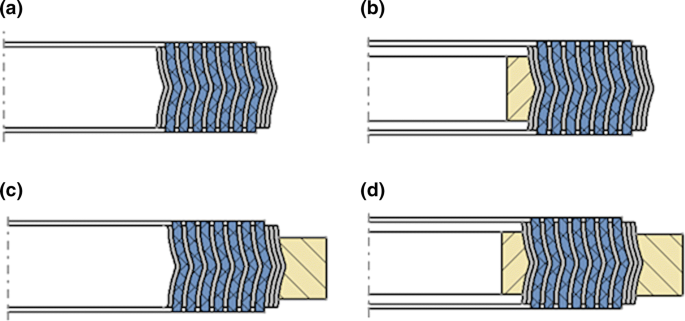
View of semi-sections of basic types of SWG; a windings only, b windings with an inner ring, c windings with an external ring, d windings with inner and outer rings
-
windings with an internal ring—Fig. 9b,
-
windings with an outer ring—Fig. 9c,
-
windings with inner and outer rings—Fig. 9d.

Each solution is dedicated to a specific shape of a flange’s face, which is schematically presented in Fig. 10. Generally, the gasket presented in Fig. 9a is used in a tongue–groove flange type (Fig. 10b) or spigot–recess flanges (Fig. 10c), where functions of the metal rings are provided by a properly shaped flange’s face.

Example of the flanges’ face solutions cooperating with given types of (SWG); a flat or raised face for gasket with two rings, b spigot–recess faces for gasket with an inner ring, c groove–tongue faces for windings only
Nevertheless, there are exceptions (due to economic reasons) where SWG presented in Fig. 9a is used in flat faces or raised faces of the flange joints. This solution is characterized by very low axial stiffness which could lead to an excessive radial deformation of the internal part of gasket’s windings, which, as a result, causes its inward buckling [20,21,22,23]. On the other hand, increased stiffness of SWG (resulting from embedding the windings in the metal rings) can lead to excessive stress of the elastic filler and its destruction or may also cause leakage growth [39]. In accordance with the standard EN 12560-2, the axial stiffness of SWG is strictly defined and it is assumed that with a bolt root stress 197 MPa or 207 MPa (depending on the flange nominal size and pressure class) the gasket should be compressed at least 20% of its initial height. The required stiffness (except for the embedded windings in the metal rings) can be achieved by means of stiffer filler (usually PTFE) or tighter winding of the tapes during the forming process [17].
According to the author’s assumption, an additional feature that can significantly influence the axial stiffness of the windings is appropriate shaping of the tapes during the production process. Therefore, in the following part of the work the process of the gasket’s optimization was carried out. It was considered that proper shaping of the metal tape leads to stress minimization in the elastic tape as well as provides the required gasket’s stiffness.
6.2 Optimization formulation
The standardized PN40 DN40 SWG without metal rings was subjected to an optimization process. The PN40 DN40 (nominal diameter 11/2”, pressure class 600) corresponds to dimensions of the standard gasket used in the tests, according to the European standard EN 13555. The set of parameters describing geometrical features of the tapes’ shape in accordance with Fig. 11 were as follows: radii of the metal tape R1 and R2, height of the metal tape h1, height of the elastic tape h2, thickness of the metal tape t1, thickness of the elastic tape t2. The material features stated as e1 corresponded to the material properties of austenitic steel of the metal tape and e2 corresponded to the material properties of CEG for the elastic tape. A set of all the described parameters of the gasket’s features were collected below:

Geometrical features of metal and elastic tapes
The radii R1 and R2 were assumed to be variable (decisive) parameters:
where R1 ϵ {0.5;2;4;8;16} mm and R2 ϵ{2;4;8;16} mm.
Constant parameters were: h1 = 4.0 mm, h2 = 4.5, t1 = 0.2 mm, t2 = 0.7 mm, material of the metal tape e1—steel 316L, material of the elastic tape e2—CEG at bulk density 0.8 g/cm3. Based on enforced conditions, an optimal design of the gasket should meet the basic criterion of achieving 20% strain of the initial gasket’s height under the bolt root stress 207 MPa and, what is more important, the strain should not cause destruction of the elastic tape. The value of bolt root stress 207 MPa in relation to the bolt dimensions of the flange joint DN40 PN40 generates pressure on the gasket’s top surface p = 80 MPa. Therefore, the criterion of optimization was formulated as follows: Find such a set of variable parameters (R1, R2), at which the equivalent stress in the elastic tape σ (s) will be minimal under windings’ strain 20% and, thus, the gasket’s contact pressure for this condition should be greater than p (s)> 80 MPa. Hence, the objective function was formulated as follows:
The first imposed constraint was:
Due to the fact that the permissible compression stress of CEG should not be exceeded, the stress in the elastic tape was imposed as a second constraint:
An additional constraint in the form of (17) was introduced in order to avoid the collapse effect of the gasket. A function of the contact pressure versus gasket’s strain p = f(ε) should be progressive in the whole range of the strain:
Ultimately, the objective function and the constraints of the gasket’s optimization were as follows:
The enforced parameter was strain ranging from 0 to 20%.
The reaction of computation was in the form of the contact pressure of the windings as well as equivalent stress in the elastic tape:
The set of parameters and reactions of SWG model are shown in Fig. 12.

The set of parameters of SWG computational model
6.3 Computational model
Figure 13 presents the axisymmetric model of the gasket (in configuration R1= 0.5 mm, R2= 4.0 mm) reflecting its location between two plates of the hydraulic press. The simulation included displacement of the upper plate from Uz= 0 to 0.9 mm, causing compression of the gasket. The value Uz = 0.9 mm constitutes 20% of the gasket’s strain at its initial height equal h2 = 4.5 mm. The lower plate of the model was fixed, whereas the upper one was set as movable in the z-axis direction. The contact area between the metal tapes and filler tapes, as well as between the plates and the gasket’s top surfaces, was set as frictional with coefficient 0.4. The mesh size of the CEG filler was 0.1 mm. The numerical issue was formulated as static with an active, nonlinear function of the material including a plastic deformation and large displacements. The discrete equation of motion was the same as (8). The upper/lower plates of the hydraulic press and the metal tape of the gasket were modeled with a steel material with Young’s modulus E = 200,000 MPa and Poisson ratio v = 0.3 (typical values of stainless steel). The plastic deformation of the metal tape was approximated by a bilinear plasticity model where the tangent modulus, after exceeding the yield stress Rp0.2 = 200 MPa, was Eu = 8000 MPa. Equation (6) presented in chapter 3 was used to model CEG’s elastic tape. The shear modulus was set as G = 15 MPa.

The axisymmetric numerical model of the windings and plates
The equation motion (8) was solved by the Newton–Raphson method. The numerical model of the gasket and plates as well as the boundary conditions is presented in Fig. 13. The calculations were divided into two basic steps. First, the initial tension of the gasket was introduced to simulate the effect of its preliminary compression resulting from the winding process. Next, the displacement of the upper plate was incrementally applied ΔUz = 0.05 mm to reach the final value Uz = 0.9 mm. Figure 14 outlines examples of the gasket’s profiles depending on the values of R1 and R2 radii.

Examples of gasket’s sections depending on the values of R1 and R2
6.4 Computational results
Figure 15 shows the distribution of the equivalent stress in the elastic tape at selected points of gasket’s compression (R1 = 0.5 mm, R2 = 2.0 mm). In compression up to 0.5 mm, the highest value of the equivalent stress in the elastic tape appeared in the vicinity of sharp edges of the metal tape. In compression ranging from 0.7 to 0.9 mm, the maximum value of the equivalent stress is located in the middle section of the structure and exactly between the first winding of the elastic and metal tapes. The course of the maximum value of the equivalent stress in the elastic tape as a function of the gasket’s strain is presented in Fig. 16a. In the initial strain phase, the stress increases in a progressive way. At the compression Uz = 0.5 mm, stress reaches the maximum value, i.e., σmax = 122 MPa. After exceeding the compression Uz> 0.5 mm stress decreased, and finally at Uz= 0.9 mm stabilized to the value σmax = 113 MPa. Figure 16b shows the course of the contact pressure as a function of the gasket’s compression. The contact pressure was calculated by dividing the reaction force (of the upper plate) by the initial top surface of the gasket. In the chart (Fig. 16b), two characteristic regions can be seen.

Distribution of the equivalent stress (MPa) in the graphite tape in subsequent deformation steps for the variant profile R1 = 0.5 mm and R2 = 2 mm; a compression 0.3 mm, b compression 0.5 mm, c compression 0.7 mm, d compression 0.9 mm

Numerical results of gasket with tape profile R1 = 0.5 mm R2 = 2 mm, a relationship of the max. equivalent stress in elastic tape versus compression of windings, b course of the contact pressure versus gasket’s strain
The first, ranging from 0 to 0.5 mm, was responsible for the compression of graphite tapes protruding beyond the metal tapes. The second, beginning from 0.5 mm, represented the moment of contact of the metal tapes with metal plates. From that point, the increment of the contact pressure strongly increased up to 0.7 mm.
When compression exceeded 0.7 mm, the contact stress increased linearly up to 0.9 mm. In the whole range of compression, the course of the function p = f (ε) is progressive. Nevertheless, the tape profile in this configuration did not meet the constraint (15), because 20% of strain occurred at the contact pressure of 65 MPa. Figure 17 presents a set of contact pressure versus gasket’s strain for the profile tape R1 = 0.5 mm and variable values of radius R2. Taking into account the imposed constraints, only the metal tape variant of R2 = 8 mm and R2 = 16 mm meets the requirement (15). However, both configurations exceed the constraint (16), since the maximum equivalent stress in the elastic tape is greater than 180 MPa (Fig. 18).

Contact pressure versus gasket strain, tape profile R1= 0.5 mm R2= var

Max. equivalent stress in elastic tape versus gasket’s strain, tape profile R1= 0.5 mm R2= var
Furthermore, characteristic p = f(ε) of the variant R2 = 16 mm in the compression range from 0.6 to 0.9 mm behaves unstably; hence, it exceeds the constraint (17). An interesting course of the characteristic p = f (ε) was observed in the variant of the tape profile R1 = 2 mm and a variable radius R2 (Fig. 19).

Contact pressure versus strain, tape profile R1= 2 mm R2= var
Except for the variants R2 = 2 mm and R2 = 4 mm, other profile configurations met the constraint (15). Nonetheless, each of them exceeded the constraint (16) σmax> 180 MPa—Fig. 20. In case of the profile tape R1 = 4 mm R2 = var, all solutions fulfill the constraint (15) (Fig. 21), whereas only two configurations R2 = 4 mm and R2 = 8 mm do not exceed the constraint (16) (Fig. 21) and the constraint (17) (Fig. 22); therefore, they meet all requirements.

Max. equivalent stress in elastic tape versus gasket’s strain, tape profile R1 = 2 mm R2= var

Contact pressure versus gasket’s strain, tape profile R1= 4 mm R2= var

Max. equivalent stress in elastic tape versus gasket’s strain, tape profile R1= 4 mm R2= var
Figure 23 shows a course of the contact pressure as a function of the gasket’s strain for tape parameters R1 = 8 mm, R2 = var. All configurations met the constraint (15). However, the courses of functions p = f (ε) of variants R2 = 8 mm and R2 = 16 mm were out of the constraint (17). Moreover, each of the variants of the tape’s profile exceeded the constraint (16) σ > 180 MPa (Fig. 24). Similar relations were obtained in case of the tape profile R1 = 16 mm, R2 = var.

Contact pressure versus windings strain, tape profile R1= 8 mm R2= var

Max. equivalent stress in elastic tape versus gasket’s strain, tape profile R1 = 8 mm R2= var
At the deformation 0.9 mm, characteristics describing the dependence of the contact pressure versus gasket’s strain practically met in one point (Fig. 25) and fulfill the limitation (15) but they exceed the limitation (17).

Contact pressure versus gasket’s strain, tape profile R1= 16 mm R2= var
Furthermore, each variant exceeded the constraint (16)—see Fig. 26. Figure 27a shows a contour plot of the maximum equivalent stress in the elastic tape as a function of parameters R1 and R2. It can be seen that the four variants fulfill the constraint (16). In Fig. 27b the contour plot of contact stress at 20% of gasket’s strain versus radii R1 and R2 is presented. Only three variants of the tape profile: (R1 = 4 mm, R2 = 4 mm), (R1 = 2, R2 = 4 mm) and (R1 = 2 mm, R2 = 8 mm) fulfilled the constraint (15). Solutions fulfilling the limitations (15), (16) and (17) are collected in Fig. 27c. It can be noticed that only one profile configuration (R1 = 4 mm, R2 = 4 mm) covers both requirements.

Max. equivalent stress in elastic tape versus gasket’s strain, tape profile R1 = 16 mm R2= var

A collection of numerical results at different gasket’s variants, a counter plot of maximum equivalent stress in graphite tape, b counter plot of contact stress acting on the gasket’s top surface at its strain 20%, c collection of tape variants which fulfills all constraints
Figure 28 presents maps of the maximum stress distribution at the characteristic points of compression of the gasket’s optimal variant R1 = 4 mm and R2 = 4 mm. Figure 29 presents a separate graph of the characteristics describing dependence of the contact pressure and the maximum stress in the elastic tape as a function of strain. The tape profile R1= 4 mm and R2 = 4 mm was finally made and tested experimentally.

Distribution of equivalent stress (MPa) in graphite tape in subsequent deformation steps for profile variants R1 = 4.0 mm and R2 = 4.0 mm; a compression 0.3 mm, b compression 0.5 mm, c compression 0.7 mm, d compression 0.9 mm

Numerical results of gasket’s tape profile R1 = 4.0 mm R2 = 4.0 mm, a relationship of the max. equivalent stress in elastic tape versus gasket’s compression, b course of the contact pressure versus gasket’s strain
6.5 Optimized SWG
In order to verify the numerical gasket’s model, the optimized variant was subjected to an experimental test. The experiment was conducted on the same test rig as presented in Fig. 6. The gasket located on the lower plate of a hydraulic press before the compression test is presented in Fig. 30. The sample was compressed up to a maximum value 0.9 mm. The experimental results in the form of the contact pressure versus gasket’s compression against the numerical results are compiled in Fig. 31. In the initial phase of compression from 0 to 0.5 mm, both curves were practically overlapping. In the compression region where the metal tape comes into contact with the press plates (from 0.5 to 0.6 mm), some differences between both compression curves were observed.

Optimized windings situated on lower plate of test rig before the compression test

Verification of numerical model of winding with optimized shape
At strain of 20% the contact pressure exerted on the gasket’s top surface was 87 MPa (in a numerical result it was 82 MPa). In the whole range of deformations, the compression curve is progressive.
7 Summary
The hyperelastic B-K model is mainly dedicated to model elastic strain energy of highly compressible elastomers which are characterized by cellular open foam. To this group of materials belongs, among others, PUF. In view of similar physical properties of CEG to PUF, the B-K model, at some assumptions, is compatible with a real deformation of CEG subjected to the compressive load. Those assumptions resulted mainly from treating CEG as an isotropic material, not plastically deformable, which in real behavior of CEG is not met. The only parameter in the B-K model depending on properties of the material was the shear modulus referring to the initial state of infinitesimal strain. In case of CEG with bulk density of 0.8 g/cm3 (experimentally verified), the best mapping of a real compressive curve was obtained at the shear modulus G = 15 MPa. The material model verified in this way was used for optimization of the spiral wound gasket. The aim of the optimization was to minimize the stress in the elastic tape and provide an adequate axial gasket’s stiffness through shaping the gasket’s cross section (consisting of metal and elastic tapes). The radii R1 and R2 describing the profile of the metal tape were assumed to be variable parameters. Twenty variants of the gasket’s configurations were taken into consideration. It was shown that there is a set of parameters (R1, R2) which met the set requirements. Generally, the increase of radius R1 leads to the increase in the gasket’s stiffness, while the decrease in radius R2 causes higher tension in the elastic tape. The optimal solution was found in the form of R1= 4 mm, R2= 4 mm. The optimized shape of the gasket was verified by experimental tests. Slight discrepancies between numerical and experimental outcomes resulted mainly from the assumed simplifications, such as treating CEG as an isotropic and fully elastic material, with no ability to dissipate energy through an internal friction as well as assuming that the friction coefficient on the cooperating surface steel-CEG equals 0.4.
8 Main conclusions of the work
-
Assuming that CEG is an isotropic and hyperelastic material, the B-K model can be used to map, with high accuracy, the deformation of CEG under axial compression.
-
A value of the material constant of the B-K model in the simulation of CEG strongly depends on the initial value of density/porosity. For modeling CEG with density of about 0.8 g/cm3, good mapping of the real compression curve was obtained at the shear modulus G = 15 MPa.
-
Modeling CEG with different density requires an experimental test to determine the correct G value.
-
The material model B-K, verified by the experimental research, provides good mapping of the deformation of the spiral wound gasket subjected to a compression load.
-
On the basis of the optimization of the spiral wound gasket, it was found that the minimal stress in the elastic tape can be achieved by adapting an appropriate shape of the cross section profile of the metal tape.
-
Decreasing radius R2 of the metal tape leads to excessive tension of the elastic tape, while the increasing radius R1 of the metal tape causes the increase in the axial stiffness of the gasket.
Abbreviations
- NG:
-
Natural graphite
- EG:
-
Expanded graphite,
- CEG:
-
Compressed expanded graphite
- PUF:
-
Polyurethane foam
- SWG:
-
Spiral wound gasket
- FEM:
-
Finite element method
- B-K:
-
Blatz–Ko material model
References
Shane H, Russel RJ, Bochman RA (1968) US Patent 3,404,061
Mortazavi B, Hassouna F, Laachachi A, Rajabpour A, Ahazi S, Chapron C, Toniazzo V, Ruch D (2013) Experimental and multiscale modeling of thermal conductivity and elastic properties of PLA/expanded graphite polymer nano-composites. Thermochim Acta 552:106–113
Gama N, Costa LC, Amaral V, Ferreira A, Barros-Timmons A (2017) Insights into the physical properties of biobased polyurethane/expanded graphite composite foams. Compos Sci Technol 138:24–31
Cho J, Luo JJ, Daniel IM (2007) Mechanical characterization of graphite/epoxy nanocomposites by multi-scale analysis. Compos Sci Technol 67:2399–2407
Kim IH, Jeong YG (2010) Polylactide/exfoliated graphite nano-composites with enhanced thermal stability, mechanical modulus, and electrical conductivity. J Polym Sci Part B 48(8):850–858
Kim LJ, Sham JM (2005) Conductive graphite nanoplatelet/epoxy nanocomposites: effects of exfoliation and UV/ozone treatment of graphite. Scripta Mater 53:235–240
Guler T, Tayfun U, Bayramli E, Dogan M (2017) Effect of expandable graphite on flame retardant, thermal and mechanical properties of thermoplastic polyurethane composites filled. Thermochim Acta 647:70–80
Fanasov IM, Savchenko DV, Ionov SG, Rusakov DA, Seleznev AN, Avdeev VV (2009) Thermal conductivity and mechanical properties of expanded graphite. Inorg Mater 45(5):486–490
Vovchenko LL, Matzui LYu, Kulichenko AA (2007) Thermal characterization of expanded graphite and its composites. Inorg Mater 43(43):597–601
Krzesinska M, Pisaroni N (2004) Mechanical properties of monolithic compressed expanded graphite-based adsorbents related to the temperature of pyrolysis and activation, studied with ultrasound. Mater Charact 52:195–202
Celzard A, Mareche JF, Furdin G (2003) Describing the properties of compressed expanded graphite through power laws. J Phys Condens Matter 15:7213–7226
Dowell MB, Howard R (1986) Tensile and compressive properties of flexible graphite foil. Carbon 24:311–323
Chung DDL (2000) Flexible graphite for gasketing, adsorption, electromagnetic interference shielding, vibration damping, electrochemical applications, and stress sensing. J Mater Eng Perform 9(2):161–163
Sorokina NE, Redchitz AV, Ionov SG, Avdeev VV (2006) Different exfoliated graphite as a base of sealing materials. J Phys Chem Solids 67:1202–1204
Veiga JC, Monteiro da Silva G, Kavanagh N (2013) Factors that influence the sealing behavior of spiral wound gasket. In: Proceedings of the ASME 2013 pressure vessel and piping division conference PVP2013 July 14–18, 2013, Paris, France
Mc Carthy J, Fitzgerald A, Reid D (2013) Spiral wound gasket compressibility and pressure ratings. In: Proceedings of the ASME 2013 pressure vessels and piping conference PVP2013, July 14–18, Paris, France
Waterland AH (2009) Analysis of the compression behavior of spiral wound gasket. In: Proceedings of the 2009 ASME pressure vessels and piping division conference July 26–30 Prague, Czech Republic, Paper No. PVP, pp 89–97
Veiga JC, Cipolatti CF, Kavanagh N, Reeves D (2011) The influence of winding density in the sealing behavior of spiral wound gaskets. In: Pressure vessels and piping conference ASME, Jan 2011, pp 103–111
Meyer R, Kolb SK Low stress/anti-buckling spiral wound gasket. International application published under the patent cooperation treaty, WO 2017/087643 A2
Attoui H, Bouzid AH, Waterland JA (2014) Buckling and lateral pressure in spiral wound gaskets. Proceedings of the ASME 20. In: Pressure vessel and piping conference 2014, Volume 2: computer technology and bolted joints, Anaheim, California, USA, July 20–24, pp 1–7
Winter JR, Leon GF (1985) Radially inward buckling of spiral wound gaskets. Am Soc Mech Eng Pressure Vessels Piping Div PVP-Vol 98:111–116
Larson RA, Bibel G (2005) Experimental and analytical evaluation of buckling forces of a spiral wound flexible gasket. In: Proceedings of the ASME pressure vessels and piping conference—computer technology, PVP-vol 2, pp 97–104
Mueller RT (1996) Recent buckling experiences with spiral wound flexible graphite filled gaskets. American society of mechanical engineers, pressure vessels and piping division PVP-Vol. 326, computer technology—applications and methodology, pp 23–34
Wang J, He QZ, Pei YY, Shi Y (2014) Effect of angle of v-type steel belt on performance of spiral wound gasket. Appl Mech Mater Adv Civil Struct Eng III 501–504:717–721
Fukuoka T, Takaki T (2003) Finite element simulation of bolt-up process of pipe flange connections with spiral wound gasket. J Pressure Vessel Technol 125(4):371–378
Abid M, Hussain S (2008) Bolt preload scatter and relaxation behaviour during tightening a 4 in-900 class flange joint with spiral wound gasket. ARCHIVE Proc Inst Mech Eng Part E J Process Mech Eng 222(2):123–134
Mathan G, Siva Prasad N (2010) Evaluation of effective material properties of spiral wound gasket through homogenization. Int J Press Vessels Pip 87:704–713
Celzard A, Mareche JF, Furdin G (2005) Modelling of exfoliated graphite. Prog Mater Sci 50:93–179
Briody C, Duignan B, Jerrams S (2011) Characterization, modelling and simulation of flexible polyurethane foam. In: International conference on materials. Tribology and recycling (MATRIB). Vela Luka, Croatia, 29 June–01 July, pp 23–36
Mane JV, Chandra S, Sharma S, Ali H, Chavan VM, Manjunath BS, Patel RJ (2017) Mechanical property evaluation of polyurethane foam under quasi-static and dynamic strain rates—experimental study. Proc Eng 173:726–731
Yonezu A, Hirayama K, Kishida H, Chen X (2016) Characterization of the compressive deformation behavior with strain rate effect of low-density polymeric foams. Polym Test 50:1–8
Ouellet S, Cronin D, Worswick M (2006) Compressive response of polymeric foams under quasi-static, medium and high strain rate conditions. Polym Test 25:731–743
Fushima S, Nagakura T, Yonezu A (2017) Experimental and numerical investigations of the anisotropic deformation behavior of low-density polymeric foams. Polym Test 63:605–613
Tu ZH, Shim VPW, Lim CT (2001) Plastic deformation modes in rigid polyurethane foams under static loading. Int J Solid Struct 38:9267–9279
Chen P, Chung DDL (2015) Elastomeric behavior of exfoliated graphite, as shown by instrumented indentation testing. Carbon 81:505–513
Blatz PJ, Ko WL (1962) Application of finite elastic theory to the deformation of rubbery materials. Trans Soc Rheol 6:223–251
Abdi M, Ashcroft I, Wildman R (2018) Topology optimization of geometrically nonlinear structures using an evolutionary optimization method. Eng Optim 50(11):1850–1870
Hartmann S (2005) A remark on the application of the Newton-Raphson method in non-linear finite element analysis. Comput Mech 36(2):100–116
Jenco JM, Hunt ES (2000) Generic issues effecting SWG performance. Int J Pressure Vessel Pip 77:825–830
Acknowledgements
Calculations have been carried out using resources provided by Wroclaw Centre for Networking and Supercomputing (http://wcss.pl), Grant No. 444.
Author information
Authors and Affiliations
Corresponding author
Additional information
Technical Editor: Paulo de Tarso Rocha de Mendonça, Ph.D.
Publisher's Note
Springer Nature remains neutral with regard to jurisdictional claims in published maps and institutional affiliations.
Rights and permissions
Open Access This article is licensed under a Creative Commons Attribution 4.0 International License, which permits use, sharing, adaptation, distribution and reproduction in any medium or format, as long as you give appropriate credit to the original author(s) and the source, provide a link to the Creative Commons licence, and indicate if changes were made. The images or other third party material in this article are included in the article's Creative Commons licence, unless indicated otherwise in a credit line to the material. If material is not included in the article's Creative Commons licence and your intended use is not permitted by statutory regulation or exceeds the permitted use, you will need to obtain permission directly from the copyright holder. To view a copy of this licence, visit http://creativecommons.org/licenses/by/4.0/.
About this article

Cite this article
Jaszak, P. Adaptation of a highly compressible elastomeric material model to simulate compressed expanded graphite and its application in the optimization of a graphite-metallic structure. J Braz. Soc. Mech. Sci. Eng. 42, 224 (2020). https://doi.org/10.1007/s40430-020-02311-8
Received:
Accepted:
Published:
DOI: https://doi.org/10.1007/s40430-020-02311-8