An Approximation Algorithm for the Stochastic Fault-Tolerant Facility Location Problem

Abstract

In this paper, we study a stochastic version of the fault-tolerant facility location problem. By exploiting the stochastic structure, we propose a 5-approximation algorithm which uses the LP-rounding technique based on the revised optimal solution to the linear programming relaxation of the stochastic fault-tolerant facility location problem.

1 Introduction

The facility location problem (FLP) has been widely studied in the operations research literature. Shmoys et al. [17] give the first constant approximation ratio of 3.16 by using the LP-rounding technique. Since then, there are several results with respect to the approximation algorithm (cf. [2, 5, 8, 9, 13]) for this problem. The currently best approximation ratio is 1.488 by Li [11] using LP-rounding combined with the technique of dual-fitting. Guha and Khuller [6] and Sviridenko [19] show that it is impossible to design an approximation algorithm with an approximation ratio less than or equal to 1.463, unless P=NP. For a discussion of the variants of the FLP, we refer to [1, 4, 22, 23] and the references therein.

The fault-tolerant facility location problem (FTFLP) is one of the most important variants of the FLP. In the setting of the FTFLP, each client is required to be assigned to more than one facility to prevent it from being out of service in case an opened facility fails. The assignment cost of each client is a weighted combination of the distances to the facilities to which the client connects. Jain and Vazirani [10] first study the FTFLP with the uniform weight and give a primal-dual algorithm with a logarithmic of the largest requirement approximation ratio. Then, Swamy and Shmoys [16] give a 2.076-approximation algorithm for the uniform weight. The approximation ratio is further improved to 1.7245 by Byrka et al. [3]. Guha et al. [7] give a 2.408-approximation algorithm for the more general non-uniform weight case. On the other hand, the stochastic facility location problem (SFLP) has also been studied extensively in the literature. Generally speaking, the SFLP contains a 2-stage stochastic process: at the first stage of the process, we are given the possible scenarios and their corresponding probability distributions, but we do not know which one will actually occur. The opening cost of each facility at different stages are different. At the second stage, the opening cost of each facility in different scenarios are different. We can open some facilities at the first stage which can serve any client in any scenario and the facilities open in a given scenario can only be used to serve clients in that particular scenario. The problem is introduced by Ravi and Sinha [14], who present an LP-rounding 8-approximation algorithm. Then, there are several results related to the SFLP (cf. [12, 15, 16, 18]). The currently best approximation ratio for the SFLP is 1.8526 by Ye and Zhang [21].

In this paper, we are interested in the stochastic fault-tolerant facility location problem (SFTFLP) in which each client in each scenario is to be assigned to more than one facility. Intuitively, some facilities may fail so that the clients require some backups. We give an LP-rounding 5-approximation algorithm by integrating the techniques of [7, 14, 17].

The organization of this paper is as follows. In Sect. 2, we describe the stochastic fault-tolerant facility location problem in detail and present its integer program model. An algorithm based on LP-rounding technique is presented in Sect. 3. Section 4 offers analysis of the algorithm. Some final remarks are given in Sect. 5.

2 The 2-Stage Stochastic Fault-Tolerant Facility Location Problem

For the 2-stage stochastic fault-tolerant facility location problem, we are given a facility set F at the first stage only. For each facility i, its opening cost is $f_{i}^{0}$ at the first stage. And also, we are given the scenario s∈{1,2,⋯,S} and the corresponding client sets D _s to be served. Assuming S is polynomial with respect to the number of facility and client, a probability p _s associated with each scenario s, and a distance function $c: F\times (\bigcup_{s}D_{s})\longrightarrow\mathbb{R}_{+}$ which is a metric, i.e., it satisfies symmetry, nonnegativity, and the triangle inequality. In each scenario s, facilities may be opened to serve the clients in D _s . The opening cost of facility i in scenario s is $f_{i}^{s}$. In each scenario s, each client j in D _s needs to be assigned to r _j distinct facilities (according to certain weights) which are opened only at the first stage and the corresponding scenario. Let the weights of assigning j to the r _j facilities be $w_{j}^{1} \geqslant w_{j}^{2} \geqslant \cdots \geqslant w_{j}^{r_{j}}$, that is, the assignment cost of client j is the weighted combination of the distance to r _j closest facilities. The goal of the problem is to assign the clients to the opened facilities such that the total expected facility open and assignment costs are minimized.

We denote $\mathcal{F}:= \{ (i, t) | i \in F, t =0, 1, \cdots , S \}$, $\mathcal{D}:= \{ (j,r,s)| s=1,\cdots ,S, j \in D_{s}, r=1,\cdots , r_{j} \}$, and ${\tilde{\mathcal{D}}}:= \{ (j, s)| s=1,\cdots ,S, j \in D_{s} \}$. Also, let p ₀:=1. We call the elements in $\mathcal{F}$ facility–scenario pair and similarly, the elements in $\mathcal{D}$ and $\tilde{\mathcal{D}}$ are called client–copy–scenario triple and client–scenario pair, respectively. For each facility–scenario pair (j,s), r∈1,2,⋯,r _j is called a copy of (j,s). Following the above notations, we can restate the problem as: given the set $\mathcal{F}$ of the facility–scenario pairs and the set $\mathcal{D}$ of the client–copy–scenario triples, we intend to open two sets of facility–scenario pairs, F ₀ at the first stage and F _s in scenario s of the second stage. At the first stage, the opening cost of facility i is $f_{i}^{0}$, and in the scenario s at the second stage, the opening cost of facility i is $p_{s}f_{i}^{s}$. And then, we need to assign each client–scenario pair to r _j distinct opened facility–scenario pair in which each client–copy–scenario triple (j,r,s) can only be assigned to the facility–scenario pairs in F ₀ and F _s , so that the total cost including the facility opening cost and the assignment cost is minimized. In order to ensure (j,r,s) cannot be assigned to the facility–scenario pair (i,t), where t≠0 and s, we define the distance between a facility–scenario pair and a client–scenario pair as follows:

$$c_{ij}^{ts} = \left \{ \begin{array}{@{}l@{\quad}l@{}} c_{ij}, & \mathrm{if}\ t=0\ {\mathrm{or}}\ s; \\ + \infty, & \mathrm{otherwise}. \end{array} \right . $$

To this end, the problem can be formulated as the following integer program.

$$ \begin{array}{l@{\quad}l@{\quad}ll} (\mathit{IP}) & \min & \sum_{(i, t) \in{\mathcal{F}} } p_t {f_i^t}{y_i^t} + \sum_{ (i, t) \in{\mathcal{F}}} \sum_{(j, r, s) \in {\mathcal{D}}} p_s w_j^r c_{ij}^{ts} x_{ij}^{tsr} \\ & \mathrm{s.t.} & \sum_{(i, t) \in{\mathcal{F}} } x_{ij}^{tsr} \geqslant 1, \quad \forall(j,r,s) \in {\mathcal{D}}, \\ & & \sum_{r=1}^{r_j} x_{ij}^{tsr} \leqslant y_i^t, \quad \forall(i, t) \in{\mathcal{F}}, \forall(j,r,s) \in{\mathcal{D}}, \\ & & x_{ij}^{tsr} \in\{ 0, 1\}, \quad \forall(j,r,s) \in{\mathcal{D}}, \\ & & y_i^t \in\{ 0, 1\}, \quad \forall(i, t) \in{\mathcal{F}}, \end{array} $$

(2.1)

in which, $y_{i}^{t}$ indicates whether the facility–scenario pair (i,t) (including t=0) is open; $x_{ij}^{tsr}$ denotes whether client j in scenario s is assigned to the facility–scenario pair (i,t) and (i,t) is the rth closest open facility–scenario pair to j. The first constraint of (2.1) requires each client–copy–scenario pair (j,r,s) should be assigned to a facility–scenario pair. The second constraint of (2.1) models that if the client–copy–scenario triple (j,r,s) is assigned to the facility–scenario pair (i,t), the pair (i,t) should open, and each facility–scenario pair (i,t) can only serve one copy of the same client–scenario pair (j,s). A solution of (2.1) indicates the set of opened facilities and the connection way of opened facilities and clients.

By relaxing the integrality constraints, we obtain the following LP relaxation:

$$\begin{aligned} \begin{array}{l@{\quad}l@{\quad}l} (\mathit{LP}) \quad & \min& \sum_{(i, t) \in{\mathcal{F}} } p_t {f_i^t}{y_i^t} + \sum_{ (i, t) \in{\mathcal{F}}}\sum_{ (j, r, s) \in {\mathcal{D}}} p_s c_{ij}^{ts} w_j^r x_{ij}^{tsr} \\ & \mathrm{s.t.} & \sum_{(i, t) \in{\mathcal{F}} } x_{ij}^{tsr} \geqslant 1, \quad \forall(j,r,s) \in {\mathcal{D}}, \\ & & \sum_{r=1}^{r_j} x_{ij}^{tsr} \leqslant y_i^t, \quad \forall(i, t) \in{\mathcal{F}}, \forall(j,r,s) \in{\mathcal{D}}, \\ & & x_{ij}^{tsr} \geqslant 0, \quad \forall(j,r,s) \in{\mathcal{D}}, \\ & & 0 \leqslant y_i^t \leqslant 1, \quad \forall(i, t) \in{\mathcal{F}}. \end{array} \end{aligned}$$

(2.2)

Let $F^{*}=\sum_{(i,t)\in\mathcal{F}} p_{t}f_{i}^{t}y_{i}^{t}$ and $C^{*}=\sum_{(i,t)\in\mathcal{F} }\sum_{(j,r,s)\in\mathcal{D}}p_{t}w_{j}^{r}c_{ij}^{ts}x_{ij}^{ts}$ be the optimal fractional facility cost and assignment cost, respectively. A feasible solution of (2.2) can be viewed as a set of fractionally opened facilities and fractional connections between opened facilities and clients.

3 The Algorithm

Now we proceed to describe the algorithm as follows.

Algorithm 3.1

(LP-Rounding Algorithm)

Step 1.:

Solving the LP relaxation and constructing a consistent solution.

• Step 1.1 Solve the LP relaxation (2.2) to obtain the optimal solution (x,y).

• Step 1.2 For each client–scenario pair $(j,s) \in{\tilde{\mathcal{D}}}$, sort all facility–scenario pairs according to their distances to (j,s) in non-decreasing order. For the same facility at the first stage and scenario s, we sort the first stage facility before the scenario one (see Fig. 1 ).

  Fig. 1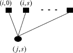

  

  Step 1.2. The circle represents the client–scenario pair (j,s). The squares represent the facility–scenario pairs which connected to (j,s)

• Step 1.3 For each client–scenario pair, we do the following process. We assign the first copy of (j,s) to the facility–scenario pair (i,t)(t=0 or s) in terms of the above ordering, i.e., we set $\bar{x}_{ij}^{ts1} : = \max \{ \min\{ y_{i}^{t}, 1 - \sum_{(i',t')\prec (i,t)} y_{i'}^{t'} \}, 0 \}$, where (i′,t′)≺(i,t) represents (i′,t′) is before (i,t) in the ordering defined in Step 1.2. For the second copy of (j,s), we start from the last facility–scenario pair to which (j,1,s) is connected and set $\bar{x}_{ij}^{ts1} : = \max\{ \min\{ y_{i}^{t}, 1 - \sum_{(i',t')\prec(i,t)} y_{i'}^{t'} \}, 0 \}$. Repeat the above process for all copies of (j,s).

  Thus, we can obtain a solution $(\bar{x},y)$ of the program (2.2) which is called a consistent solution.

Step 2.:

Filtering and scaling.

For each client–scenario pair (j,s), we run the following operations in the increasing order of copies r=1,2,⋯,r _j . For each client–copy–scenario triple (j,r,s), sort the facility–scenario pairs in non-decreasing order of their distances to (j,r,s)(same as Step 1). Then, we set $C_{j}^{sr} := c_{i^{*}j}^{t^{*}sr}$, where (i ^∗,t ^∗) is the first pair such that $\sum_{(i,t): c_{ij}^{ts}\leqslant c_{i^{*}j}^{t^{*}s}}{\bar{x}_{ij}^{tsr}}\geqslant \frac{2}{5}$. We also set

$$\hat{x}_{ij}^{tsr} : = \left \{ \begin{array}{@{}l@{\quad}l@{}} \bar{x}_{ij}^{tsr} & \mathrm{if}\ c_{ij}^{ts}<C_{j}^{sr}; \\ \frac{2}{5}-\sum_{(i,t):c_{ij}^{ts}<c_{i*j}^{t*s}} \hat{x}_{ij}^{tsr} &\mathrm{if}\ c_{ij}^{ts}=C_{j}^{sr}; \\ 0 & \mathrm{otherwise}. \end{array} \right . $$

Furthermore, we scale $\hat{x}_{ij}^{tsr}$ by $\frac{5}{2}$ to obtain $\tilde{x}_{ij}^{tsr}$ such that $\sum_{(i,t)}\tilde{x}_{ij}^{tsr}=1$. For the feasibility, we let $\tilde{y}_{i}^{t} : =\min\{\frac{5}{2} y_{i}^{t},1\}$.

Step 3.:

Clustering.

For ease of exposition, we denote

$$\begin{aligned} F_{0}(j,r,s) : =&\bigl\{ (i,0)|\tilde{x}_{ij}^{0sr}>0 \bigr\} , \\ F_{s}(j,r,s) : =&\bigl\{ (i,s)| \tilde{x}_{ij}^{ssr}>0 \bigr\} , \\ w_{0}(j,r,s) : =&\sum_{(i,0)\in F_{0}(j,r,s)} \tilde{x}_{ij}^{0sr}, \\ w_{s}(j,r,s) :=& \sum_{(i,s)\in F_{s}(j,r,s)} \tilde{x}_{ij}^{ssr}. \end{aligned}$$

Let $\bar{\mathcal{D}}$ denote the set of the unassigned client–copy–scenario triples which will be updated in the clustering process. Initially, $\bar{\mathcal{D}} : = \mathcal{D}$ contains all the client–copy–scenario triples. For each client–copy–scenario triple (j,r,s), let $\bar{C}(j,r,s)$ denote the facility–scenario pair set which serves (j,r,s) according to the solution $(\tilde{x}, \tilde{y})$.

• Step 3.1 Picking center.

  Arrange all client–copy–scenario triples in non-decreasing order of the values of $C_{j}^{sr}$, that is, $C_{j}^{rs} := \sum_{(i,t)} c_{ij}^{ts} \tilde{x}_{ij}^{tsr}$. Assume (j,r,s) has the smallest $C_{j}^{sr}$ in $\bar{\mathcal{D}}$, which we call a center.

• Step 3.2 Choosing facility–scenario pair set.

  Choose F _t (j,s,r), where $t = \arg\max_{\bar{t} = \{ 0,k\} } \{w_{\bar{t}}(j,r,s)\}$. Let N _F (j,r,s) and Y be the facility–scenario pair set which will be assigned to the center (j,r,s) and the sum of the values of the facility–scenario pairs in N _F (j,r,s), respectively. Given a value of Y, partition (i,t) means partitioning (i,t) into (i ₁,t) and (i ₂,t) such that $\tilde{y}_{i_{1}}^{t}:=w_{t}(j,r,s)$ and $\tilde{y}_{i_{2}}^{t}:=Y-\tilde{y}_{i_{2}}^{t}$, while maintaining $\sum_{r}\tilde{x}_{ij}^{tsr}\leqslant \tilde{y}_{i}^{t}$ for both i=i ₁ and i=i ₂.

  • Step 3.2.1 Initially, set N _F (j,r,s):=∅ and Y:=0.

  • Step 3.2.2 Let $(i',t) := \arg\min_{(i,t)\in F_{t}(j,r,s)}p_{t}f_{i}^{t}$ and set $Y:=\tilde{y}_{i'}^{t}$, F _t (j,r,s):=F _t (j,r,s)−{(i′,t)}, and N _F (j,r,s):={(i′,t)}. If Y>w _t (j,r,s), partition (i′,t).

  • Step 3.2.3 If Y⩽w _t (j,r,s), we check whether Y is exactly w _t (j,r,s) or not. If Y=w _t (j,r,s), we can obtain a facility–scenario pair N _F (j,r,s). If Y<w _t (j,r,s), we choose a facility–scenario pair (i,t) in F _t (j,r,s) arbitrarily and set $Y:=Y+\tilde{y}_{i}^{t}, F_{t}(j,r,s):=F_{t}(j,r,s)- \{(i,t)\}$. After that, it is possible that Y>w _t (j,r,s). For this, partition (i,t) into (i ₁,t) and (i ₂,t), and set N _F (j,r,s):=N _F (j,r,s)∪{(i ₁,t)}, $Y:=Y-\tilde{y}_{i_{2}}^{t}$. Otherwise, set N _F (j,r,s):=N _F (j,r,s)∪{(i,t)} and check whether the value of Y is bigger than w _t (j,r,s) again as above.

  • Step 3.2.4 We can obtain a facility–scenario pair set N _F (j,r,s) of a center (j,r,s) whose value is w _t (j,r,s) exactly.

• Step 3.3 Choosing client–copy–scenario triple set and reassigning other copies of the chosen client–scenario pair.

  For each remaining client–scenario pair (j′,s′), we denote

  $$R\bigl(j',s'\bigr): =\bigl\{ r|\exists(i,t) \in N_{F}(j,r,s), \ \mathrm{s.t.}\ \tilde{x}_{ij'}^{ts'r}>0 \bigr\} . $$

  Assume R(j′,s′)={r ₁,r ₂,⋯,r _k(j′,s′)}. Then, N _D (j,r,s):=⋃ _{R(j′,s′)≠∅} {(j′,r ₁,s′)} and $\bar{\mathcal{D}}:=\bar{\mathcal{D}}-N_{D}(j,r,s)$.

  It is necessary to deal with the remaining copies of (j′,s′). Initially, T(j′,r ₁,s′) is the facility–scenario pair set which serves (j′,r ₁,s′) but not in N _F (j,r,s), that is, $T(j',r_{1},s'):=\bar{C}(j',r_{1},s')-N_{F}(j,r,s)$. For a client–copy–scenario triple (j′,r _m ,s′), set $X:=\sum_{(i,t)\in N_{F}(j,r,s)}\tilde{x}_{ij'}^{ts'r_{m}}$. Then, check whether X is exactly 0 or not. If it is true, we turn to the next copy. Otherwise, let $(\tilde{i},\tilde{t}): = \arg \min_{(i,t)\in T(j',r_{1},s')} c_{ij'}^{ts'r_{1}}$. If $X>\tilde{y}_{\tilde{i}}^{\tilde{t}}$, set $\tilde{x}_{\tilde{i}j'}^{\tilde {t}s'r_{m}}:=\tilde{y}_{\tilde{i}}^{\tilde{t}}$, $T(j',r_{1},s'):=T(j',r_{1},s')-\{(\tilde{i},\tilde{t})\}$, and $X:=X-\tilde{x}_{\tilde{i}j'}^{\tilde{t}s'r_{m}}$; Otherwise, set $\tilde{x}_{\tilde{i}j'}^{\tilde{t}s'r_{m}}:=X$, $\tilde{y}_{\tilde{i}}^{\tilde{t}}:=\tilde{y}_{\tilde{i}}^{\tilde{t}}-X$, and $X:=X-\tilde{x}_{\tilde{i}j'}^{\tilde{t}s'r_{m}}$. Finally, for all (i,t)∈N _F (j′,r ₁,s′), set $\tilde{x}_{ij'}^{ts'r_{m}}:=0$.

• Step 3.4 Constructing cluster.

  We call {(j,r,s),N _F (j,r,s),N _D (j,r,s)} a cluster centered by (j,r,s). Update $\mathcal{D} := \mathcal{D} \setminus( N_{D}(j,r,s) \cup\{(j,r,s)\} )$.

  Repeat the above procedure until each client–copy–scenario triple belongs to some cluster.

Step 4.:

Rounding.

We can obtain several disjoint clusters at the end of Step 3. In each cluster, we open the cheapest facility–client pair and close the others, and assign each client–copy–scenario triple to the opened facility–scenario pair.

We illustrate the process of clustering (Step 3 of Algorithm 3.1) in Figs. 2, 3, 4, 5.

Fig. 2

Picking center

Fig. 3

Choosing facility–scenario pair set

Fig. 4

Choosing client–copy–scenario triple set

Fig. 5

Constructing cluster

4 Analysis

In this section, we analyze the relationship between the costs corresponding to the primal feasible solution (x,y) and the solution obtained from Algorithm 3.1, which results in the approximation ratio. We first clarify that Algorithm 3.1 is well-defined before proceeding to the analysis of the approximation ratio. In our analysis, we use fraction to represent the value of the variables, $\tilde{x}_{ij}^{tsr}$ or $\tilde{y}_{i}^{t}$. In Algorithm 3.1, we construct a solution in step 2 which should be feasible. Note that a consistent solution satisfies the following.

• The set of facilities to which the triple (j,r _k(1),s) is fractionally assigned are closer to (j,s) than any facility to which the triple (j,r _k(2),s) is fractionally assigned for 1⩽r _k(1)<r _k(2)⩽r _j and $(j,s) \in{\mathcal{D}}$.

• For each facility–scenario pair (i,t) and client–scenario pair (j,s) in the consistent solution, there exist at most two copies of (j,s) which are assigned to (i,t) simultaneously. Furthermore, if two such copies exist, then they must be consecutive.

Then the following lemma accounts for its feasibility.

Lemma 4.1

The solution $(\tilde{x},\tilde{y})$ obtained from step 2 of Algorithm 3.1 is a feasible solution to (LP).

Proof

Obviously, the first constraint of (LP) holds for $(\tilde{x}, \tilde{y})$ from the construction process. Then, we need to show $\sum_{r=1}^{r_{j}}\tilde{x}_{ij}^{tsr}\leqslant \tilde{y}_{i}^{t}$. Therefor, we consider the following cases.

• Case 1. If the facility–scenario pair (i,t) is assigned to just one client–copy–scenario triple, it is trivial.

• Case 2. From the property of the consistent solution, we know there are at most two copies which are assigned to the same facility–scenario pair. Therefore, we assume that (j,r,s) and (j,r+1,s) are assigned to (i,t) (note t=0 or s).

  • Case 2.1. If $y_{i}^{t}\leqslant \frac{2}{5}$, it is true before scaling. Therefore, it is also true after scaling by the same factor.

  • Case 2.2. If $y_{i}^{t}>\frac{2}{5}$, note that if we can show $\hat{x}_{ij}^{tsr}+\hat{x}_{ij}^{tsr+1}\leqslant \frac{2}{5}$, then the lemma holds. Since (i,t) is the farthest distance to (j,r,s) among those assigned facility–scenario pairs in the solution of $(\bar{x},y)$, it is easy to see that $\hat{x}_{ij}^{tsr}=\max\{0,\bar{x}_{ij}^{tsr}-\frac{3}{5}\}$.

    • Case 2.2.1. If $\hat{x}_{ij}^{tsr}=0$, then $\hat{x}_{ij}^{tsr+1}\leqslant \frac{2}{5}$ from the scaling process.

    • Case 2.2.2. If $\hat{x}_{ij}^{tsr}=\bar{x}_{ij}^{tsr}-\frac{3}{5}$, then $\hat{x}_{ij}^{tsr}+\hat{x}_{ij}^{tsr+1}\leqslant \bar{x}_{ij}^{tsr}+\bar{x}_{ij}^{tsr+1}-\frac{3}{5}\leqslant \frac{2}{5}$.

 □

In the third step of Algorithm 3.1, assume that we reassign (j′,r ₂,s′),(j′,r ₃,s′),⋯,(j′,r _k(j′,s′),s′) to the facility–scenario pairs which was assigned to (j′,r ₁,s′) in solution of $(\tilde{x}, \tilde{y})$. It is necessary to analyze the feasibility of this operation. Similar as [7], assuming that (j′,r ₁,s′) belongs to the cluster centered by the client–copy–scenario triple (j,r,s), we compute $I_{j'}^{s'1} = \sum_{(i,t) \in N_{F}(j,r,s)}{\tilde{x}_{ij'}^{ts'r_{1}}}$ which denotes the sum of the fraction of (j′,r ₂,s′) connected to the facility–scenario pair in N _F (j,r,s), and $I_{j'}^{s'2}$, $I_{j'}^{s'3}, \cdots, I_{j'}^{s'k(j',s')}$ in the similar manner. We define $O_{j'}^{s'1}=1-I_{j'}^{s'1}$, and $O_{j'}^{s'2}$, $O_{j'}^{s'3}, \cdots, O_{j'}^{s'k(j',s')}$ similarly. From the above definition, we can obtain the following lemma directly.

Lemma 4.2

For any (j′,u,s′) which is fractionally assigned to the facilities in set N _F (j,r,s), we have

$$I_{j'}^{s'u}+O_{j'}^{s'u}=1 \quad \mathrm{for}\ \mathrm{all}\ 1\leqslant u\leqslant k, \quad \mathrm{and} \quad \sum _{u=1}^{k(j',s')}{I_{j'}^{s'u}}\leqslant \sum _{(i',t)\in N_{F}(j,r,s)}{\tilde{y}_{i'}^{t}}. $$

Based on Lemma 4.2, we can show the feasibility of reassignment as follows.

Lemma 4.3

For any client–scenario pair (j′,s′), we can always reassign the copies r ₂, r ₃, ⋯, r _k(j′,s′) to T(j,r ₁,s) where (j,r,s) is the center of the cluster which (j,r ₁,s) belongs to and the cost of the reassignment will not increase.

Proof

Note that since $(\tilde{x},\tilde{y})$ is also a consistent solution, the cost cannot be increasing if we reassign (j′,r ₂,s′),⋯,(j′,r _k(j′,s′),s′) to the facility–scenario pair which was previously assigned to (j′,r ₁,s′).

In order to prove the feasibility of Algorithm 3.1, we should show that it is always possible to do the reassignment, that is, the sum of the fractions of client–copy–scenario triple (j′,r″,s′)(r″ is from r ₂ to r _k (j′,s′)) served by N _F (j,r,s) is no more than the total fraction of (j′,r ₁,s′) served by T(j′,r ₁,s′). By Lemma 4.2 and the construction of the cluster, we have $I_{j'}^{s'1}+O_{j'}^{s'1}=1$ and $\sum_{u=1}^{k(j',s')}I_{j'}^{s'u}\leqslant 1$. Thus, it is clear that $\sum_{u=2}^{k(j',s')}I_{j'}^{s'u}\leqslant O_{j'}^{s'1}$. □

So far, the algorithm has been proven to obtain a feasible integer solution for the SFTFLP. The next step is to calculate the ratio of the costs associated with the feasible solution and optimal solution.

Lemma 4.4

If $\tilde{x} _{ij}^{tsr}>0$, then $c_{ij}^{ts}\leqslant \frac{5}{3}{C_{j}^{sr}}$.

Proof

Since $\tilde{x}_{ij}^{tsr}>0$, we can obtain $\bar{x}_{ij}^{tsr}>0$. From the way of choosing (i ^∗,t ^∗), (i ^∗,t ^∗) has the farthest distance to (j,r,s). Moreover,

$$c_{i^*j}^{t^*s}\leqslant \frac{\sum_{(i,t):c_{ij}^{ts}\geqslant c_{i^*j}^{t^*s}}{c_{ij}^{ts}\bar{x}_{ij}^{tsr}}}{\sum_{(i,t):c_{ij}^{ts}\geqslant c_{i^*j}^{t^*s}}{\bar{x}_{ij}^{tsr}}}\leqslant \frac{5}{3}C_{j}^{sr}. $$

 □

From the process of Algorithm 3.1, we have the following theorem:

Theorem 4.5

Algorithm 3.1 is a polynomial-time 5-approximation algorithm for the SFTFLP.

Proof

Since the processes of filtering, scaling, and clustering can be implemented in polynomial time, we know that Algorithm 3.1 is a polynomial-time algorithm. We consider the facility cost and the assignment cost of the solution obtained by Algorithm 3.1, respectively.

First, we consider the expected facility cost. We denote the set of all cluster centers in Algorithm 3.1 as $\hat{\mathcal {D}}$. For any cluster center $(j,r,s)\in\hat{\mathcal{D}}$.

Case 1. If we choose F ₀(j,r,s), implying that $w_{0}(j,r,s) \geqslant \frac{1}{2}$, the facility–scenario pair in N _F (j,r,s) is formed (i,0). The expected facility cost incurred by (j,r,s) is bounded by

$$\begin{aligned} \frac{\sum_{(i,0)\in N_{F}(j,r,s)} f_{i}^{0}\tilde{y}_{i}^{0} }{w_{0}(j,r,s)} \leqslant & \frac{5}{2w_{0}(j,r,s)} \sum_{(i,0)\in N_{F}(j,r,s)} f_{i}^{0}y_{i}^{0} \\ \leqslant & 5 \sum_{(i,0)\in N_{F}(j,r,s)} f_{i}^{0}y_{i}^{0}. \end{aligned}$$

Case 2. If we choose F _s (j,r,s), implying that $w_{0}(j,r,s) \geqslant \frac{1}{2}$, the facility–scenario pair in N _F (j,r,s) is formed (i,s). The expected facility cost incurred by (j,r,s) is bounded by

$$\begin{aligned} \frac{\sum_{(i,s)\in N_{F}(j,r,s)} f_{i}^{s}\tilde{y}_{i}^{s} }{w_{s}(j,r,s)} \leqslant & \frac{5}{2w_{s}(j,r,s)} \sum_{(i,s)\in N_{F}(j,r,s)} f_{i}^{s}y_{i}^{s} \\ \leqslant & 5 \sum_{(i,s)\in N_{F}(j,r,s)} f_{i}^{s}y_{i}^{s}. \end{aligned}$$

Because the clusters are disjoint, we can obtain an upper bound for the total expected facility cost

$$E \biggl[ 5\sum_{(j,r,s)\in\hat{\mathcal{D}}}{\sum _{(i,t)\in N_{F}(j,r,s)}{p_{t}f_{i}^{t} y_{i}^{t}}} \biggr] \leqslant 5\sum_{(i,t)\in\mathcal{F}}{p_{t}f_{i}^{t}y_{i}^{t}}. $$

Second, we consider the assignment cost of client $(j',r',s')\in \mathcal{D}$. If $(j',r',s')\in\hat{\mathcal{D}}$, the assignment cost can be bounded by $\frac{5}{3}C_{j}^{sr}$ by Lemma 4.4. Otherwise, for the center of the cluster to which (j′,r′,s′) belongs, denote the center as (j,r,s) and the opened facility–scenario pair as (i,t)∈N _F (j,r,s). Since (j′,r′,s′) is assigned to (i,t) finally, there exits a facility–scenario pair (i′,t′) such that $\tilde{x}_{i'j}^{t'sr}>0$ and $\tilde{x}_{i'j'}^{t's'r'}>0$, also that (i′,t′)∈N _F (j,r,s). By the triangle inequality, we can obtain

$$c_{ij'}^{ts'r'} \leqslant c_{i'j'}^{t'r's'} + c_{i'j}^{t'sr} + c_{ij'}^{ts'r'} \leqslant \frac{5}{3}\bigl(2C_{j}^{sr}+C_{j'}^{s'r'} \bigr) \leqslant 5 C_{j'}^{s'r'}, $$

in which the last inequality holds since (j′,r′,s′) is a center. Therefore, the assignment cost is bounded by $5\sum_{(j,r,s)\in\mathcal{D}} C_{j}^{sr}$.

By summing up the expectation of the facility cost and the assignment cost, the expected total cost can be bounded by

$$5 \biggl( \sum_{(i,t)\in\mathcal{F}}{p_{t}f_{i}^{t}y_{i}^{t}}+ \sum_{(j,r,s)\in\mathcal{D}}p_{s}w_{j}^{r} C_{j}^{sr} \biggr) =5\bigl(F^*+C^*\bigr). $$

It follows that the approximation ratio of Algorithm 3.1 is 5. □

5 Concluding Remarks

In this paper, we considered the stochastic fault-tolerant facility location problem and gave a 5-approximation algorithm using the LP-rounding technique. In the future, it would be interesting to consider improvement of the approximation ratio for the problem. Moreover, it is valuable to design approximation algorithm for the capacitated version of stochastic fault-tolerant facility location problem.

References

Ageev, A., Ye, Y., Zhang, J.: Improved combinatorial approximation algorithms for the k-level facility location problem. SIAM J. Discrete Math. 18, 207–217 (2004)
Byrka, J., Aardal, K.I.: An optimal bifactor approximation algorithm for the metric uncapacitated facility location problem. SIAM J. Comput. 39, 2212–2213 (2010)
Bykra, J., Srinivasan, A., Swamy, C.: Fault-tolerant facility location: a randomized dependent LP-rounding algorithm. In: Proc. of IPCO, pp. 244–257 (2010)
Chen, X., Chen, B.: Approximation algorithms for soft-capacitated facility location in capacitated network design. Algorithmica 53, 263–297 (2007)
Chudak, F.A., Shmoys, D.B.: Improved approximation algorithms for the uncapacitated facility location problem. SIAM J. Comput. 33, 1–25 (2003)
Guha, S., Khuller, S.: Greedy strike back: improved facility location algorithms. J. Algorithms 31, 228–248 (1999)
Guha, S., Meyerson, A., Munagala, K.: A constant factor approximation algorithm for the fault-tolerant facility location problem. J. Algorithms 48, 429–440 (2003)
Jain, K., Mahdian, M., Markakis, E., Saberi, A., Vazirani, V.V.: Greedy facility location algorithm analyzed using dual fitting with factor-revealing LP. J. ACM 50, 795–824 (2003)
Jain, K., Vazirani, V.V.: Approximation algorithms for metric facility location and k-median problems using the primal-dual schema and Lagrangian relaxation. J. ACM 48, 274–296 (2001)
Jain, K., Vazirani, V.V.: Approximation algorithms for fault tolerant metric facility location problem. Algorithmica 38, 433–439 (2003)
Li, S.: A 1.488-approximation algorithm for the uncapacitated facility location problem. In: Proc. of ICALP, Part II, pp. 77–88 (2011)
Mahdian, M.: Facility location and the analysis of algorithms through factor-revealing programs. Ph.D. thesis, MIT, Cambridge, MA (2004)
Mahdian, M., Ye, Y., Zhang, J.: Approximation algorithms for metric facility location problems. SIAM J. Comput. 36, 411–432 (2006)
Ravi, R., Sinha, A.: Hedging uncertainty: approximation algorithms for stochastic optimization programs. Math. Program. 108, 97–114 (2006)
Shmoys, D.B., Swamy, C.: An approximation scheme for stochastic linear programming and its application to stochastic integer programs. J. ACM 53, 978–1012 (2006)
Shmoys, D.B., Swamy, C.: Fault-tolerant facility location. ACM Trans. Alg. 4, Article No. 51 (2008)
Shmoys, D.B., Tardös, E., Aardal, K.I.: Approximation algorithms for facility location problems (extended abstract). In: Proc. of STOC, pp. 265–274 (1997)
Srinivasan, A.: Approximation algorithms for stochastic and risk-averse optimization. In: Proc. of SODA, pp. 1305–1313 (2007)
Sviridenko, M.: Cited as personal communication in Chudak and Shmoys [5] (1998)
Wu, C., Xu, D., Shu, J.: An LP rounding approximation algorithm for the stochastic fault-tolerant facility location problem. In: Proc. of ISORA, pp. 164–169 (2011)
Ye, Y., Zhang, J.: An approximation algorithm for the dynamic facility location problem. In: Cheng, M., Li, Y., Du, D. (eds.) Combinatorial Optimization in Communication Networks, pp. 623–637. Kluwer Academic, Dordrecht (2005)
Zhang, J.: Approximating the two-level facility location problem via a quasi-greedy approach. Math. Program. 108, 159–176 (2006)
Zhang, P.: A new approximation algorithm for the k-facility location problem. Theor. Comput. Sci. 384, 126–135 (2007)
Acknowledgements
The authors would like to thank the two anonymous referees for many helpful suggestions.
Author information
Authors and Affiliations
Corresponding author
Additional information
C. Wu was supported by National Natural Science Foundation of China (Grant No. 11071268). D. Xu was supported by National Natural Science Foundation of China (Grant No. 11371001), Scientific Research Common Program of Beijing Municipal Commission of Education (Grant No. KM201210005033), and China Scholarship Council. J. Shu was supported by National Natural Science Foundation of China (Grant Nos. 70801014, 71171047, and 71222103).
An extended abstract of this paper appeared in Wu et al. [20].
Rights and permissions
About this article
Cite this article
Wu, C., Xu, D. & Shu, J. An Approximation Algorithm for the Stochastic Fault-Tolerant Facility Location Problem. J. Oper. Res. Soc. China 1, 511–522 (2013). https://doi.org/10.1007/s40305-013-0034-7
Received:
Revised:
Accepted:
Published:
Issue Date:
DOI: https://doi.org/10.1007/s40305-013-0034-7