PolyProc: A Modular Processing Pipeline for X-ray Diffraction Tomography

Abstract

Direct imaging of three-dimensional microstructure via X-ray diffraction-based techniques gives valuable insight into the crystallographic features that influence materials properties and performance. For instance, X-ray diffraction tomography provides information on grain orientation, position, size, and shape in a bulk specimen. As such techniques become more accessible to researchers, demands are placed on processing the datasets that are inherently “noisy,” multi-dimensional, and multimodal. To fulfill this need, we have developed a one-of-a-kind function package, PolyProc, that is compatible with a range of data shapes, from planar sections to time-evolving and three-dimensional orientation data. Our package comprises functions to import, filter, analyze, and visualize the reconstructed grain maps. To accelerate the computations in our pipeline, we harness computationally efficient approaches: for instance, data alignment is done via genetic optimization; grain tracking through the Hungarian method; and feature-to-feature correlation through k-nearest neighbors algorithm. As a proof-of-concept, we test our approach in characterizing the grain texture, topology, and evolution in a polycrystalline Al–Cu alloy undergoing coarsening.

Introduction

The microstructures of materials, from ceramics to superalloys, are three-dimensional (3D) in nature. Such materials are opaque to most probes, and hence, they have been traditionally studied by two-dimensional (2D) techniques, e.g., optical or electron microscopy. By coupling the image capture with microstructure sectioning, 3D characterization is possible [1,2,3,4]. Unfortunately, however, serial sectioning entails the removal of consecutive layers of material to collect 2D images, and so this method is fundamentally destructive. Instead, nondestructive metrologies are needed to detect various microstructural features (e.g., grains and precipitates) and monitor their evolution with a sufficient temporal resolution. For this purpose, X-ray imaging techniques enable the direct visualization of 3D microstructure in a nondestructive manner, since X-rays can penetrate deeply in the materials investigated. Computed tomography (CT) is one of the oldest 3D imaging [5] techniques that make use of an X-ray beam. As the transmitted X-rays are sensitive to the density of the material, the resulting 3D microstructure shows density differences through the illuminated sample. This is the basis of absorption CT (denoted as ACT). On the other hand, analysis of the diffracted X-ray beam is the hallmark of 3D X-ray diffraction (3DXRD) [6,7,8,9,10,11,12]. Thus, X-ray microscopes capable of diffraction provide a unique opportunity to characterize polycrystalline materials in 3D.

Recognizing the promise of 3DXRD, investigators in the past decade have developed a number of different 3DXRD techniques, such as high-energy X-ray diffraction microscopy (HEDM) [9], diffraction contrast tomography (DCT) [8, 10, 12], and scanning 3DXRD (S3DXRD) [11], to name a few. These techniques are all based on X-ray diffraction, and thus, they share common features in terms of their working principle: As a “hard” (≧ 10 keV) X-ray beam illuminates a specimen, a detector placed behind the sample collects diffraction patterns (spots or streaks) that are generated when grains in the microstructure satisfy the Bragg condition. To track the locations of all grains within the tomographic field-of-view, the specimen is rotated with a small angular increment (≲ 2°). The diffraction images collected must then be segmented or partitioned into two classes (streak and background). The segmented diffraction streaks are then indexed as grains through a reconstruction procedure, such as the GrainMapper3D algorithm used here. Differences in the 3DXRD techniques stem from the shapes and sizes of incident X-ray beam, chromaticity of source, resolution of detector, and means of reconstruction [13].

Until recently, nondestructive grain mapping via 3DXRD was only available at synchrotron facilities with limited accessibility. With the recent development of laboratory-based X-ray diffraction tomography (denoted as LabDCT), bulk polycrystalline specimens can now be readily characterized from one’s own laboratory [12, 14, 15], spearheading a new age in 3D materials science. Unlike synchrotron-based DCT, LabDCT makes use of a polychromatic, divergent beam, thereby requiring a different reconstruction procedure. A number of studies have already demonstrated the efficacy of LabDCT for the high-throughput characterization of polycrystalline microstructures [16,17,18,19]. For instance, Keinan et al. [16] integrated ACT and LabDCT imaging modalities on a single X-ray microscope to gain new insight into the microstructure of metallurgical-grade polycrystalline silicon, which is simultaneously multi-phase and polycrystalline. McDonald et al. [18] conducted 3D space- and time-resolved experiments via both LabDCT and ACT to investigate the dynamics of sintering of micrometer-scale Cu particles. While great strides have been made in technique development and applications, a critical need exists to devise the infrastructure for processing such high-dimensional and multimodal datasets.

To this end, a few software packages have been developed to aid in the processing of reconstructed X-ray images. Here, we review the strengths and limitations of a few. TomoPy is a Python-based, open-source framework for the reconstruction and analysis of absorption images in particular [20]. As of this writing, the software has not been extended to support 3DXRD data, which is inherently multi-dimensional. That is, 3DXRD provides orientational information (a vector quantity) for each voxel in the imaging domain. At the other extreme is MTEX, a free MATLAB toolbox for analyzing the crystallographic texture from vectorized orientation data outputted from diffraction-based techniques such as electron backscatter diffraction [21]. However, MTEX cannot as yet handle the processing of 3D grain maps. In contrast, DREAM.3D is a software package that allows for the construction of customized workflows to analyze 3D orientation data, including serial sectioning, DCT, and HEDM [22]. While DREAM.3D has demonstrated success in processing 3DXRD data, it has not been optimized for high-dimensional datasets. Thus, the question remains, “How does one 3D microstructure relate to the next in a dynamic experiment?” To answer this question, we present our efforts in developing a data processing pipeline, PolyProc, capable of parsing the full spectrum of 2D, 3D, and further higher-dimensional data collected through 3DXRD techniques. With our toolbox, it is also possible to “layer” one dataset over another, thereby providing a unified description of the underlying microstructure.

Experiment

Herein, we demonstrate the efficacy of our function package with two full-field (volume) scans that are separated by a short time-interval. In this interval, we apply an external stimulus (heat) to encourage the coarsening of grains in the microstructure. We collect the 3D data through the LabDCT module in a laboratory X-ray microscope (Zeiss Xradia 520 Versa) located at the Michigan Center for Materials Characterization at the University of Michigan. We selected an alloy of composition Al–3.5 wt% Cu for subsequent analysis, as it is relatively well characterized and does not attenuate the incident X-ray beam too heavily. The sample was prepared for the first round of imaging by annealing at 485 °C, thereby achieving a fully recrystallized state. Of note is that this temperature is below the solvus temperature (about 491 °C), and thus, we retained secondary θ-Al₂Cu particles within the system. Annealing also releases the strain accumulated in the cold-rolled condition. From our experience, strain has the effect of smearing the diffraction spots of polycrystals. This, in turn, introduces difficulties in reconstruction, since it becomes impossible to “untangle” the overlapping diffraction spots belonging to individual grains in the microstructure. Following the annealing, the specimen was imaged through LabDCT, collecting 181 projection images every ~ 2° between 0° and 360° with an exposure time of 400 s per projection. The detector images measure 385 μm of the sample from top to bottom. Due to the nondestructive nature of LabDCT, we further annealed the same sample for four minutes at the aforementioned temperature (485 °C), inducing the microstructural evolution. The second round of imaging was done with the same scan conditions. The specimen was annealed further and imaged in ACT on the same microscope to acquire the spatial distribution of secondary phase θ-Al₂Cu particles within the tomographic field-of-view. In the ACT scan, we collected 1600 projections evenly distributed between 0° and 180° with an exposure of 5.3 s. The Cu constituent provided a natural source of attenuation contrast such that the θ-Al₂Cu particles could be readily identified via ACT.

The LabDCT diffraction patterns were segmented and reconstructed via the GrainMapper3D™ software developed by Xnovo Technology ApS. In the reconstruction, the volume is overlaid on a structured grid with side length of 5 μm. Based on the known crystal symmetry and lattice parameters, the equations of diffraction are solved for a subset of spots in order to compute a prospective orientation. Then, the forward simulations calculated by the software are compared against the real grains reflection on the detector. A grain is said to be indexed when a match is found between the reflection observed on the detector and predicted position from the forward simulation. Figure 1 shows superposition of the two. The color of calculated diffraction spot represents the crystallographic orientation of grains that give rise to the various spots. Overall, good agreement is seen between the reconstructed and measured results; the simulated patterns are able to capture not only the position of the spots but also their shapes. The software outputs the high-dimensional data in the hierarchical data format version 5 (HDF5), which was designed for complex data objects. Each voxel in the 3D image domain contains the following attributes: its grain identification, Rodrigues vector (texture components), and completeness value. On the other hand, the ACT dataset was directly reconstructed using the filtered back-projection algorithm employed by the Scout and Scan software on the Zeiss Xradia 520 microscope. Our principal task is to process this high-dimensional and heterogeneous data, as will be described in detail below.

Fig. 1

Superposition of experimental and calculated diffraction patterns, the latter obtained from forward modeling the reconstruction data. A beam-stop (center) blocked the forward-transmitted beam. Color of calculated spots in the periphery reflects crystallographic orientation of the diffracting grain according to the standard triangle. White scale bar is 1000 μm

The GrainMapper3D reconstructions are inherently six-dimensional (i.e., 3D space plus 3D orientation). For matrix algebra and plotting, we use the MATLAB R2018a programming language, which provides a high-level technical computing environment. Our toolbox takes advantage of a few different toolkits that are freely distributed through MathWorks, such as MTEX (described above) [21]. MTEX is required to run the pipelines involving data clustering, crystallographic analysis, and grain tracking. Other dependencies are included as utilities within the toolbox.

Result and Discussion

This section demonstrates integral procedures for processing and analyzing in situ and 3D crystallographic datasets. A typical workflow of the function package is illustrated in Fig. 2, organized in a set of modules that group the algorithms according to their function. In time-dependent studies (like ours), there is likely a misalignment of the scanned domains and/or grain orientations between consecutive time-steps, causing challenges in data analysis downstream. Thus, after importing the HDF5 data, our workflow starts with the alignment of volume data via genetic optimization to define the common scope (intersection volume) for further analysis. Within the defined scope, grain cleanup procedures filter unreliable features such as incorrectly indexed voxels that inevitably appear during data collection. The grains are processed according to three thresholds: angular, volumetric, and completeness. The cleaned data can be visualized in 3D or cross-sectionally in 2D with different color schemes depending on user preference. Data analysis functions provide various capabilities for the statistical analysis of the entire polycrystalline aggregate or a single grain in particular. Additionally, for time-resolved data, our toolbox offers a means of grain tracking via combinatorial optimization. We step through each of these modules using the two LabDCT reconstructions as a test case.

Fig. 2

Workflow for processing 3D LabDCT data; see text for details

Data Processing

Volume Alignment

A geometric deviation of sample, including translation and rotation, would be found between two time-steps (denoted $t_{1}$ and $t_{2}$ hereafter) if the sample was to be repeatedly removed and mounted on its holder. Translation will introduce a spatial drift in the corresponding grains between the two datasets. Meanwhile, rotation will alter the perceived crystallographic orientation of the grains between time-steps $t_{1}$ and $t_{2}$. Both transformations will thereby mislead further analysis like grain tracking. Thus, body alignment (registration) of sample volume is the first step of our pipeline.

We solve the registration problem by minimizing the misfit of volume through genetic algorithm (GA). Volume is defined as the set of all pixels within the 3D sample; misfit is the number of voxels not shared between the two volumes $t_{1}$ and $t_{2}$, over total number of voxels. Six independent parameters are determined during the alignment procedure: three translational vectors $\left( {T_{x} , T_{y} , T_{z} } \right)$ and three rotational angles $\left( {R_{x} , R_{y} , R_{z} } \right)$, assuming a purely isometric transformation. This implies a massive calculation over a 6D space to calculate and compare misfit, if done for all possible transformations. Instead, we achieve a better alignment in a much shorter amount of compute time via GA. The detailed operating principle of GA is discussed below. After those six parameters are optimized by GA, a transformation matrix is generated for the alignment of $t_{2}$ onto $t_{1}$, where $t_{1}$ is the reference state. The application of the obtained transformation matrix on scalar data is illustrated in Fig. 3a, where volumes $t_{1}$ and $t_{2}$ are presented by blue and red colors, respectively. Before alignment (top left), a huge misfit is observed. After alignment (top center), not only the outermost contour of sample volume, but also the orientation and location of a pore inside the volume (see arrow) align closely. Subsequently, the shared (intersection) volume is determined (top right), which serves as a “mask” to ensure that all the following comparisons between $t_{1}$ and $t_{2}$ are carried out under the same region-of-interest.

Fig. 3

Procedures for a registering sample volume and defining its intersection; and b updating crystallographic orientation of grains based on the rotation angles obtained from volume alignment. Arrows in top and bottom rows point to features that are registered between the datasets $t_{1}$ and $t_{2}$. Scale bar measures 100 μm

Based on the Euler rotation matrix described by three rotational angles $\left( {R_{x} , R_{y} , R_{z} } \right)$, the crystallographic orientation of grains is also updated. Figure 3b shows the registration of grain orientations. Color represents crystallographic orientation parallel to the specimen height ($z$-direction). It can be found that crystallographic orientation of grains becomes similar after updating their Rodrigues vectors. For example, the grains indicated by white arrows are a pair of matching grains. The orientation of those two matched grains is presented by cyan and green colors before updating orientations, respectively. Once the Rodrigues vectors are updated, the grain color at $t_{2}$ becomes cyan (bottom right), which corresponds closely to the grain at $t_{1}$. To quantify the accuracy of the orientation alignment, we calculated the change of average misorientation of the matching grains between time-steps. Before the orientation update, average misorientation angle of the matching grains is 7.56 ± 0.13°; after the update, it decreases to 2.63 ± 0.59°.

Since volume alignment is only evaluated by the degree of misfit, it can be formulated as an optimization problem. GA has a few advantages over other optimization engines. For instance, it is generally effective in optimizing a function with many local minima since it does not require a good starting estimate; furthermore, it is quite flexible in that it places no constraint on the form of the objective function [23, 24]. Due to these merits, GA has been employed to register 2D and 3D data [24,25,26]. In this work, GA function from Global Optimization Toolbox of MATLAB is employed [27]. Drawing from Darwin’s theory of natural selection, GA begins with a randomly generated set of individuals (rigid transformations in our case) also known as a population at first generation (see Fig. 4). Parallel computation is utilized to calculate the fitness (here, misfit) between transformed volume at $t_{2}$ and volume at $t_{1}$. Individuals with relatively lower misfit would then be selected from the current population and its genome modified and recombined to produce the next generation. We set the maximum number of generations to 25, although this may require some tuning based on the size of the search space. Once the lowest misfit computed lies below the user-specified misfit tolerance during the 25 generations, the algorithm is interrupted in order to output the corresponding six parameters. If the calculated misfit never goes under the threshold, another iteration of GA with 25 generations containing twice the population size is triggered. Larger population size gives more opportunity to reach global minima rather than local minima. Finally, GA outputs the six parameters corresponding to the lowest misfit. As GA is “embarrassingly parallel” and converges to a high-quality solution after only a few generations through a number of bio-inspired operators, the computation time is low and accuracy of alignment is quite high. In practice, parent selection is done by stochastic universal sampling; mutation via Gaussian distribution; and crossover through scattered blending. Further details regarding GA can be found in Ref. [27]. In contrast, it is difficult to optimize the accuracy of “brute force” calculations due to the limitation of finite search step size. The accuracy and efficiency were compared on a workstation with Intel(R) Xeon(R) E-2176 M CPU core and 64 GB RAM capacity. Between volumes $t_{1}$ and $t_{2}$, the angular constraints were set to ± 7° for each of the three rotational angles $\left( {R_{x} , R_{y} , R_{z} } \right)$ and misfit tolerance of 2%, for both GA and “brute force” comparison approach. The former took 657 s for body alignment with 2.42% of misfit, while the latter took 1175 s with 2.61% misfit. The result indicates that GA can significantly improve the automated registration of 3DXRD data, achieving a better alignment in a much shorter amount of time.

Fig. 4

Mechanism of automated volume alignment via genetic algorithm (GA). Individuals from the later time-step are generated and mutated, and their misfit is calculated accordingly. Shown is a single generation of GA. The algorithm proceeds by selecting those individuals with the highest fitness (lowest misfit) for the next generation (not pictured)

Grain Cleanup

The cleanup module aims to align the data based on outputted transformation matrices (from above) and further process them to exclude unreliable features within the intersection volume. Upon importing the raw (i.e., as-collected) 3DXRT data together with alignment matrices and mask array, data outside of masked scope are cropped, and every dimension of data except orientation is transformed to the new frame-of-reference. Since the calculation of crystal orientation is computationally costly—there are ${\text{O}}\left( {N^{3} } \right)$ rotations that need to be performed, assuming a mask dimension of $N$—the Rodrigues vectors are updated only after the average orientation of grain is computed based on clustering voxels with similar orientation. That is, based on a user-defined angular threshold (typically ≤ 1°), grains with very small misorientation angles are grouped into a single grain. This order of operations greatly reduces computation load without compromising the accuracy of orientational alignments.

After clustering grains and updating the average grain orientations, data are further processed to remove small grains. Any grain composed of fewer voxels than a preset volume threshold is considered as noise and treated as unindexed regions. The rationale behind this procedure is to retain statistically significant grains and not to artificially inflate grain statistics. The volume threshold is determined based on the spatial resolution of the reconstruction data (10 μm for LabDCT). Finally, grains with lower average completeness than a preset completeness threshold are considered as unreliable data and marked as unindexed. Low-completeness grains are often located near the edges of the LabDCT aperture, wherein grains may lie partially outside of the illuminated field-of-view. Consequently, their diffraction patterns are partially occluded by the aperture, resulting in a low reconstruction completeness in forward modeling simulations.

Outputs of this module include basic measurements of the processed grains: Grain volume is expressed as total number of voxels; grain orientation as the average Rodrigues vector over all voxels in each grain; grain position as its center-of-volume, considering the Euclidean coordinates of every voxel in the grain. Grain adjacency is also stored in a form of a $M$ by 2 arrays of neighboring pairs that meet at a grain boundary, where $M$ is the number of unique pairs. Those grains adjacent to the free surfaces of the sample are designated as “exterior” grains and those in the bulk as “interior.”

Visualization

The segmented grain surfaces are meshed or represented as a series of triangles and vertices. Triangulation is accomplished via MATLAB’s built-in Marching Cubes routine. To eliminate any “staircasing” artifacts that occur as a result of the triangulation, we smooth the mesh to better reflect the physical grain shape. In particular, we make use of Laplacian smoothing, which utilizes the normalized curvature operator as weights for smoothing in a direction normal to the mesh interface. In practice, we apply only a few iterations of mesh smoothing in order to reduce artifacts while preserving the integrity of the interface.

Different modes for mesh coloring are available based on user preference. For instance, the grains can be colored according to their crystallographic orientation, topology (i.e., number of grain neighbors), volume, and average completeness. Figure 5 illustrates these different representations of the $t_{1}$ volume. It should be noted that average completeness value of many grains is close to 0.45 because reconstruction of this particular dataset was executed with a tolerance level of 0.45, meaning that indexing voxels concluded once a completeness value of 0.45 was achieved. Grains located on the topmost surface of the sample show a lower completeness compared to ones located below because those grains partially lie out of the illuminated field-of-view. The bottom surface of the sample is not shown because it is outside the intersection mask between volumes $t_{1}$ and $t_{2}$ (see also Fig. 3a). Visualization of individual 2D slices along the specimen z-direction is also available under the same color schemes, thereby demonstrating the versatility of our function package in handling different data shapes.

Fig. 5

Visualization of 3DXRD data in 2D and 3D. Grain color corresponds to a crystallographic orientation, b number of neighboring grains, c grain volume, d average completeness of grain. Scale bar measures 100 μm

Data Analysis

Simple Metrics

Direct imaging of 3D microstructure allows for the characterization of various indicators of microstructure evolution, including grain size, shape, and topology. These metrics can only be estimated via quantitative stereology of planar sections [28]. To our benefit, these parameters can be measured directly from 3DXRD without any averaging or interpolation. In the analysis module, we provide some basic statistics at the grain level. These include

• Grain volume, see, e.g., Fig. 6a corresponding to $t_{1}$ volume. A wide range of grain sizes is captured in the grain size distribution, from 33 voxels (4.3 × 10³ μm³) to 20,298 voxels (2.5 × 10⁶).

  Fig. 6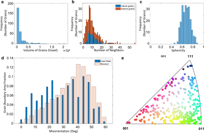

  

  Analysis of 267 grains in the microstructure. a Grain size distribution, b neighbors distribution, c sphericity distribution, d misorientation distribution (i.e., Mackenzie plot), and e inverse pole figure where colors are drawn from the standard triangle. Shown in d for comparison is the distribution expected for a material with uniformly distributed misorientations

• Grain topology, Fig. 6b. An accurate assessment of topology is limited by the finite sample size [29], meaning that the number of neighbors for the “exterior” grains may be underestimated compared to those in the specimen “interior.” To resolve this potential bias, we distinguish between topologies of “interior” versus “exterior” grains.

• Grain morphology, Fig. 6c. Sphericity ($\varPsi$) is defined as a ratio of surface area of a sphere having the same volume of a grain to the actual surface area of a grain; that is, $\varPsi = \frac{{\pi ^{{\frac{1}{3}}} \left( {6V_{g} } \right)^{{\frac{2}{3}}} }}{{A_{g} }},$ where $V_{g}$ is volume of a grain and $A_{g}$ is surface area of a grain. The former is outputted from above, while the latter is determined as the summation of each triangle area adorning the grain surfaces, $A_{g} = \mathop \sum \nolimits_{i = 1}^{F} A_{tri}^{i}$, where $A_{tri}^{i}$ is the area of triangle $i$ and $F$ is the total number of triangle faces. The area of each triangle is computed as $A_{{tri}}^{i} = \frac{1}{2}\left\| {\overset{\lower0.5em\hbox{$\smash{\scriptscriptstyle\rightharpoonup}$}}{e} _{12}^{i} \times \overset{\lower0.5em\hbox{$\smash{\scriptscriptstyle\rightharpoonup}$}}{e} _{13}^{i}} \right\|$, where $\overset{\lower0.5em\hbox{$\smash{\scriptscriptstyle\rightharpoonup}$}}{e}_{jk}^{i}$ is the edge vector from vertex $j$ to $k$ of triangle $i$. The vast majority of grains at the time-step $t_{1}$ show a relatively high compactness ($\varPsi \to 1$), which is expected for a recrystallized system.

• Grain misorientation, Fig. 6d. Misorientation $\Delta g$ is formally defined as $\Delta g = g_{i} g_{j}^{T}$, where $g_{i}$ and $g_{j}$ are the grain average orientations (in Rodrigues vectors) determined from the cleanup module above. The histogram weights in the misorientation distribution are the grain boundary areas, found by summing over all triangle areas along the boundary. We show for comparison the distribution expected for a material with uniformly distributed misorientations. The results for the $t_{1}$ data indicate a near-random distribution of grain boundaries.

• Grain texture, Fig. 6e. Shown is the inverse pole figure (IPF) of all grains in the $t_{1}$ volume. It can be seen that the sample has no obvious texture at this particular time-step.

Multimodal Analysis

The integration of multiple imaging modalities enables us to investigate correlations between various features, thereby providing an in-depth understanding of the underlying microstructure. For instance, in the multimodal analysis module, we correlate the positions of grain boundaries (retrieved via LabDCT) to that of secondary features (observed via ACT). The ACT data are assumed to be registered to the LabDCT data through application of the functions in the alignment module. The secondary features are (in our case) micrometer-scale θ-Al₂Cu particles whose locations in the microstructure are given in the form of centroid coordinates. The user may specify a grain-of-interest (GOI) and a distance threshold to then determine which particles in the particle cloud are adjacent to the GOI, and the corresponding grain-to-particle distances. We visualize the particles within a two-voxel distance threshold in Fig. 7a. To link grain boundaries to secondary features, we have developed a new algorithm, summarized here as follows: (1) For each triangle face along the grain boundaries, we calculate its centroid; next (2) we find the nearest-neighbor distances between the face centroid and particle locations; and (3) if this distance is less than the threshold, we conclude that the particle lies on or sufficiently close to the triangle face.

Fig. 7

Analysis of a single grain according to its a adjacency to secondary features (here, $\theta$-Al₂Cu precipitates in red), and b misorientation with adjacent grains. Only those particles within two voxels of the grain boundary surfaces are shown. The one voxel “gap” between two given grain faces in b arises due to the uncertainty of classifying that voxel to a given face. Scale bar measures 50 μm. c Particle-associated misorientation distribution of the same grain. Volume fraction of particles adjacent to grain boundaries is shown in blue, and Mackenzie plot is shown in orange

Step (2) above can be accomplished by calculating the Euclidean distance between each particle and each mesh triangle and then organizing the results in the ascending order of distance. This approach would necessitate $N \times M$ calculations to correlate particle and grain boundary positions, where $N$ is the number of particles and $M$ the number of mesh triangles that enclose a given grain. Considering that $M$ is on the order of 10⁵ and $N$ is also 10⁵ (this work), the task of particle classification (as near or far from the boundary) is computationally intensive if done in such an exhaustive manner. To recognize patterns in the locations of particles with respect to grain boundaries, we harness the $k$-nearest neighbors ($k$-NN) algorithm, a type of “lazy” learning. $k$-NN lessens the computational load significantly—determining the nearest-neighbor particles in seconds—by using a so-called $K$ d-tree to narrow the search space. This algorithm was previously implemented in measuring the local velocities of solid–liquid interfaces in dynamic, synchrotron-based CT experiments [30].

Provided that the grain misorientations are known (Fig. 7b), we can measure the particle-associated misorientation distribution (PMDF), among other interrelationships [31]. The PMDF is defined as the fraction of secondary features (here, particles) that are located on or in the vicinity of grain boundaries within a specific range of misorientation angles. It can be seen in Fig. 7c that the distribution of particles does not follow the distribution of grain boundaries, which might be expected if the particle–boundary correlations were truly random (i.e., density of particles per unit area of boundary is constant).

Grain Tracking

In this module, we define a mapping between experimental time-steps, allowing for the analysis of individual grains as time progresses. We use two key parameters for grain tracking: crystallographic misorientation and physical distance. The crystallographic orientation of a given grain should not change over time, provided the sample is fully recrystallized, and its location within the microstructure should also not change too drastically. Figure 8 illustrates our approach for grain tracking. Under the above two constraints, we search for a matching grain at some time-step in the future ($t + \Delta t$) within a local neighborhood of the grain at the current time-step $t$. The neighborhood is defined as the smallest cuboid that encapsulates a grain with a user-defined additional padding (in number of voxels). Any grain included in the cuboidal scope is considered to be within a local neighborhood. For instance, the gray-colored region in Fig. 8 illustrates the cuboidal scope of grain $m$ with default padding of two voxels. Care must be taken in defining the size of the grain neighborhood since too large a padding may lead to an incorrect grain assignment and too small an extension may fail to contain the matching grain. Any grain that is partially contained in this cuboidal scope at time-step $t + \Delta t$ is labeled as a candidate grain.

Fig. 8

a Mechanism of grain tracking. For the candidate grains $n$ in the neighborhood of grain $m,$ physical distances $\Delta d_{nm}$ and misorientation angles $\Delta \theta_{nm}$ are computed. These parameters are combined linearly to give the cost of assignment according to Eq. 1. The green line represents the matching grain among other candidate grains (red lines). b Schematic of cost matrix $\varvec{J}$, where row and column entries represent grains from time-step $t$ and $t + {{\Delta }}t$, respectively. Colored entries in each row represent candidate grains at $t + {{\Delta }}t$; color scheme indicates cost of assignment. c Output binary matrix, $\varvec{X}$, where row and column entries represent grains from time-step $t$ and $t + {{\Delta }}t$ (as before). Black-colored entries are optimized assignments

For each candidate grain in the neighborhood, we tabulate its distance and misorientation. Distance $\Delta d_{nm}$ refers to that between the centroid of grain $m$ and centroid of candidate grain $n$. The maximum (threshold) distance is predetermined as the half-diagonal length of cuboidal neighborhood. Similarly, misorientation angle $\Delta \theta_{nm}$ is that between grain $m$ at time-step $t$ and grain $n$ at time-step $t + \Delta t$. The maximum allowable misorientation (threshold) is a user-defined value. In theory, the misorientation between two datasets should be zero if the sample is perfectly registered and there are no grain rotations. Yet this is often not the case due to slight misalignments between datasets (see “Data Processing” section). These two metrics are combined linearly to formulate a cost function $J_{nm}$ associated with the assignment of grain $n$ to grain $m$,

$$J_{nm} = c \Delta d_{nm} + \left( {1 - c} \right)\Delta \theta_{nm} ,$$

(1)

where $c$ is a scalar quantity (ranging from zero to one) that reflects the importance of the distance over misorientation criterion. Rohrer uses a similar formulation of the cost function [32]. The problem of grain tracking is then to find the lowest cost way of assigning grains from one time-step to the next. To solve this assignment problem in polynomial time, we employ the Hungarian algorithm (otherwise known as the Kuhn–Munkres algorithm) [33, 34]. The algorithm operates on a cost matrix $\varvec{J} = \left\{ {J_{nm} } \right\}_{N \times M}$ and outputs a binary matrix $\varvec{X} = \left\{ {x_{\text{nm}} } \right\}_{{{\text{N}} \times {\text{M}}}}$, where $x_{nm} = 1$ if and only if the $n$th grain at $t$ is assigned to the $m$th grain at $t + {{\Delta }}t$. The total cost is then found as $\mathop \sum \nolimits_{i = 1}^{N} \mathop \sum \nolimits_{j = 1}^{M} x_{\text{nm}} J_{nm} \to { \hbox{min} }.$ Unlike the typical assignment problem with a square cost matrix (i.e., the matrix dimensions are such that $N = M$), our cost matrix is rectangular ($N < M$) since the total number of grains decreases with time over the course of grain growth. However, the algorithm can be extended to rectangular arrays using the method prescribed by Ref. [34], which we have applied here. Worth mentioning is that the cost element $J_{nm}$ for a non-candidate grain is computed to infinity, preventing the assignment of disappearing grains. Elements for candidate grains are normalized by threshold values to bring orientation and distance parameters into the same scale.

The result of grain tracking via Hungarian algorithm approach is evaluated using two performance metrics, matching efficiency and computation time. Matching efficiency represents the percentage of grains that are successfully tracked (assigned), i.e.,

$${\text{matching}}\;{\text{efficiency}}\;(\% ) = \frac{{{\text{number}}\;{\text{of}}\;{\text{matched}}\;{\text{grains}}\;{\text{at}}\;{\text{later}}\;{\text{time}}\;{\text{step}}}}{{{\text{number}}\;{\text{of}}\;{\text{total}}\;{\text{grains}}\;{\text{at}}\;{\text{later}}\;{\text{time}}\;{\text{step}}}}\times 100$$

(2)

Grain tracking between the two LabDCT datasets achieved a ~ 86% matching efficiency. The remaining ~ 14% of grains that were not assigned can be mainly attributed to grains that emerged into the tomographic field-of-view. Since the rod specimen is long enough to be considered an open system, “new” grains that were not captured in previous time-step may be detected near the top and bottom of the X-ray source aperture. This can be confirmed from Fig. 3b that top layer of $t_{2}$ volume has several new grains that are not observed in previous $t_{1}$ volume.

Hungarian optimization offers distinct advantages over the “brute force” solution to the assignment problem. The latter considers every possible assignment, implying a complexity of ${\text{O}}\left( {N!} \right)$. To speed up the task at hand, we may elect to iteratively (i) locate a grain neighborhood, (ii) compute costs $J_{nm}$ of all grains in the neighborhood and (iii) assign matching grains based on minimum cost; once a matching grain is found, we proceed to the next grain in the dataset. However, rather than computing cost matrices $\varvec{J}$ and analyzing the matching problem in a comprehensive manner, this approach sequentially assigns matching grain as it goes through the N grains, causing an inherent bias from the matching order. It is for this reason that the Hungarian algorithm offers a higher matching accuracy and computational efficiency over these brute force methods. On a same workstation with Intel(R) Xeon(R) E-2176 M CPU core and 64 GB RAM, grain tracking between datasets with $M = 308$ and $N = 295$ grains via Hungarian optimization takes 11.44 s with a cuboidal scope padding of two voxels, misorientation threshold of four degrees, and weight factor c of zero. On the other hand, the three-step iterative matching scheme described above takes 15.69 s with the same parameters and offers a matching rate of ~ 85%. Even though the matching efficiency of both methods is comparable, tracking by brute force results in a few cases of incorrect assignments for the reasons mentioned above. Even larger data sizes (e.g., fine-grained materials) should widen the performance gap between combinatorial optimization and “brute force” approaches.

Conclusion

With the concomitant rise and accessibility of 3D characterization approaches, there is an emerging need for processing the multimodal and multi-dimensional data outputted from such techniques. To this end, we have developed a set of functions to import, process, and analyze 3DXRD datasets of varying dimensions, from 2D to higher dimensions. Through effective computational routines, the toolbox allows us to align and track features in a highly accurate, efficient, and robust manner. For instance, we have achieved a 45% decrease in computation time by registering data via genetic optimization. Similarly, we attained an 86% matching rate between grains in consecutive time-steps, whereas brute force solution to the assignment problem achieved a similar matching efficiency in 37% longer time. Our package also includes functions to filter out unreliable features of the experimental data, perform basic statistics on the “cleaned” data, and visualize the resultant microstructures. We also offer a solution to correlate and fuse the results from different imaging modalities and/or instruments, e.g., ACT and LabDCT. The full breadth of our toolbox is tested on two datasets of a bulk metallic specimen undergoing grain growth, yet the toolbox is capable of processing a stream of multiple datasets. It is also noteworthy that the toolbox is not strictly limited to metals nor coarsening phenomena, as showcased here. Rather, we expect that our function package will provide a cross-cutting foundation for data processing involving very minimal sample-specific tuning. Potential test cases include studies of crack propagation in polycrystalline materials, embrittlement of grain boundaries, and defects in additively manufactured polycrystals.

Our function package is available as a free and open-source MATLAB toolbox and may be downloaded from repository platforms, such as Github (https://github.com/shahaniRG/PolyProc) and MATLAB File Exchange (https://www.mathworks.com/matlabcentral/fileexchange/71829-polyproc). It is open to any party wishing to not only use the codes but also contribute to its vitality. Current efforts in code development are directed toward merging data from DCT and HEDM experiments. While both techniques fall under the bracket of 3DXRD (see Introduction), they offer a different granularity of analysis. At the one extreme, HEDM has been shown to capture intragranular orientation spreads in severely deformed materials [35]. Unfortunately, the high-quality results come at the expense of the long scanning and analysis times. This is because HEDM uses a layer-by-layer approach (somewhat akin to serial sectioning). Conversely, DCT uses a “box” beam that illuminates the full sample at once, and therefore, one can collect data at a faster rate than with HEDM. However, the discretization unit in DCT reconstruction is the entire grain, much larger than the pixel size in HEDM. By collecting only a few data “slices” via HEDM, however, one can interpolate orientation spreads over the full DCT volume. For this purpose, deep learning (through, e.g., convolutional neural networks) will be necessary.

References

Rowenhorst DJ, Gupta A, Feng CR, Spanos G (2006) 3D Crystallographic and morphological analysis of coarse martensite: combining EBSD and serial sectioning. Scr Mater 55:11–16. https://doi.org/10.1016/j.scriptamat.2005.12.061
Uchic MD, Holzer L, Inkson BJ, Principe EL, Munroe P (2007) Three-dimensional microstructural characterization using focused ion beam tomography. Mater Res Soc Bull 32:408–416. https://doi.org/10.1557/mrs2007.64
Rowenhorst DJ, Lewis AC, Spanos G (2010) Three-dimensional analysis of grain topology and interface curvature in a β-titanium alloy. Acta Mater 58:5511–5519. https://doi.org/10.1016/j.actamat.2010.06.030
Groeber MA, Haley BK, Uchic MD, Dimiduk DM, Ghosh S (2006) 3D reconstruction and characterization of polycrystalline microstructures using a FIB-SEM system. Mater Charact 57:259–273. https://doi.org/10.1016/j.matchar.2006.01.019
Hounsfield GN (1973) Computerized transverse axial scanning (tomography): part 1. Description of system. Br J Radiol 46:1016–1022. https://doi.org/10.1259/0007-1285-46-552-1016
Lauridsen EM, Schmidt S, Suter RM, Poulsen HF (2001) Applied crystallography tracking: a method for structural characterization of grains in powders or polycrystals. J Appl Cryst 34:744–750. https://doi.org/10.1107/s0021889801014170
Poulsen HF (2012) An introduction to three-dimensional X-ray diffraction microscopy. J Appl Cryst 45:1084–1097. https://doi.org/10.1107/s0021889812039143
Ludwig W et al (2009) New opportunities for 3D materials science of polycrystalline materials at the micrometre lengthscale by combined use of X-ray diffraction and X-ray imaging. Mater Sci Eng A 524:69–76. https://doi.org/10.1016/j.msea.2009.04.009
Suter RM, Hennessy D, Xiao C, Lienert U (2006) Forward modeling method for microstructure reconstruction using x-ray diffraction microscopy: single-crystal verification. Rev Sci Instrum 77:123905. https://doi.org/10.1063/1.2400017
Johnson G, King A, Honnicke MG, Marrow G, Ludwig W (2008) X-ray diffraction contrast tomography: a novel technique for three-dimensional grain mapping of polycrystals. II. The combined case. J Appl Cryst 41:310–318. https://doi.org/10.1107/s0021889808001726
Hayashi Y, Hirose Y, Seno Y (2015) Polycrystal orientation mapping using scanning three-dimensional X-ray diffraction microscopy. J Appl Cryst 48:1094–1101. https://doi.org/10.1107/s1600576715009899
King A, Reischig P, Adrien J, Peetermans S, Ludwig W (2014) Polychromatic diffraction contrast tomography. Mater Charact 97:1–10. https://doi.org/10.1016/j.matchar.2014.07.026
Renversade L et al (2016) Comparison between diffraction contrast tomography and high-energy diffraction microscopy on a slightly deformed aluminium alloy. IUCrJ 3:32–42. https://doi.org/10.1107/s2052252515019995
McDonald SA et al (2015) Non-destructive mapping of grain orientations in 3D by laboratory X-ray microscopy. Sci Rep 5:14665. https://doi.org/10.1038/srep14665
Holzner C et al (2016) Diffraction contrast tomography in the laboratory-applications and future directions. Microsc Today 24:34–43. https://doi.org/10.1017/s1551929516000584
Keinan R, Bale H, Gueninchault N, Lauridsen EM, Shahani AJ (2018) Integrated imaging in three dimensions: providing a new lens on grain boundaries, particles, and their correlations in polycrystalline silicon. Acta Mater 148:225–234. https://doi.org/10.1016/j.actamat.2018.01.045
Sun J et al (2019) Grain boundary wetting correlated to the grain boundary properties: a laboratory-based multimodal X-ray tomography investigation. Scr Mater 163:77–81. https://doi.org/10.1016/j.scriptamat.2019.01.007
Mcdonald SA et al (2017) Microstructural evolution during sintering of copper particles studied by laboratory diffraction contrast tomography (LabDCT). Sci Rep 7:5251. https://doi.org/10.1038/s41598-017-04742-1
Sun J et al (2017) 4D study of grain growth in armco iron using laboratory x-ray diffraction contrast tomography. IOP Conf Ser Mater Sci Eng. https://doi.org/10.1088/1757-899x/219/1/012039
Gürsoy D, Carlo DF, Xiao S, Jacobsen C (2014) TomoPy: a framework for the analysis of synchrotron tomographic data. J Synchrotron Rad 21:1188–1193. https://doi.org/10.1107/s1600577514013939
Bachmann F, Hielscher R, Schaeben H (2010) Texture analysis with MTEX-free and open source software toolbox. Solid State Phenom 160:63–68. https://doi.org/10.4028/www.scientific.net/SSP.160.63
Groeber MA, Jackson MA (2014) DREAM.3D: a digital representation environment for the analysis of microstructure in 3D. Integr Mater Manuf Innov 3:5. https://doi.org/10.1186/2193-9772-3-5
Goldberg DE, Holland JH (1988) Genetic algorithms and machine learning. Mach Learn 3:95–99. https://doi.org/10.1023/a:1022602019183
Chow CK, Tsui HT, Lee T (2004) Surface registration using a dynamic genetic algorithm. Pattern Recognit 37:105–117. https://doi.org/10.1016/s0031-3203(03)00222-x
Lomonosov E, Chetverikov D, Ekárt A (2005) Pre-registration of arbitrarily oriented 3D surfaces using a genetic algorithm. Pattern Recogn Lett 27:1201–1208. https://doi.org/10.1016/j.patrec.2005.07.018
Brunnstrom K, Stoddart AJ (1996) Genetic algorithms for free-form surface matching. Proc Int Conf Pattern Recogn. https://doi.org/10.1109/icpr.1996.547653
Goldberg DE (1989) Genetic algorithms in search, optimization & machine learning. Addison-Wesley, Boston
Underwood EE (1973) Quantitative stereology for microstructural analysis. In: McCall JL, Mueller WM (eds) Microstructural analysis. Springer, Boston, pp 35–66
DeHoff RT, Aigeltinger EH, Craig KR (1972) Experimental determination of the topological properties of three-dimensional microstructures. J Microsc 95:69–91. https://doi.org/10.1111/j.1365-2818.1972.tb03712.x
Shahani AJ, Xiao X, Skinner K, Peters M, Voorhees PW (2016) Ostwald ripening of faceted Si particles in an Al–Si–Cu melt. Mater Sci Eng A 673:307–320. https://doi.org/10.1016/j.msea.2016.06.077
Roberts CG, Semiatin SL, Rollett AD (2007) Particle-associated misorientation distribution in a nickel-base superalloy. Scripta Mater 56:899–902. https://doi.org/10.1016/j.scriptamat.2007.01.034
Bhattacharya A, Shen YF, Hefferan CM, Li SF, Lind J, Suter RM, and Rohrer GS (2019) Three-dimensional observations of grain volume changes during annealing of polycrystalline Ni. Acta Mater 167:40–50. https://doi.org/10.1016/j.actamat.2019.01.022
Kuhn HW (1955) The Hungarian method for the assignment problem. Nav. Res. Logist. Q. 2:83–97. https://doi.org/10.1002/nav.3800020109
Bourgeois F, Lassalle JC (2002) An extension of the Munkres algorithm for the assignment problem to rectangular matrices. Commun ACM 14:802–804. https://doi.org/10.1016/j.imavis.2008.04.004
Lind J et al (2014) Tensile twin nucleation events coupled to neighboring slip observed in three dimensions. Acta Mater 76:213–220. https://doi.org/10.1016/j.actamat.2014.04.050
Acknowledgements
We gratefully acknowledge financial support from the Army Research Office Young Investigator Program under award no. W911NF-18-1-0162. We also acknowledge the University of Michigan College of Engineering for financial support and the Michigan Center for Materials Characterization for use of the instruments and staff assistance.
Author information
Authors and Affiliations
Corresponding author
Ethics declarations
Conflict of interest
The authors declare that they have no conflicts of interest.
Rights and permissions
Open Access This article is licensed under a Creative Commons Attribution 4.0 International License, which permits use, sharing, adaptation, distribution and reproduction in any medium or format, as long as you give appropriate credit to the original author(s) and the source, provide a link to the Creative Commons licence, and indicate if changes were made.
The images or other third party material in this article are included in the article’s Creative Commons licence, unless indicated otherwise in a credit line to the material. If material is not included in the article’s Creative Commons licence and your intended use is not permitted by statutory regulation or exceeds the permitted use, you will need to obtain permission directly from the copyright holder.
To view a copy of this licence, visit http://creativecommons.org/licenses/by/4.0/.
About this article
Cite this article
Kang, J., Lu, N., Loo, I. et al. PolyProc: A Modular Processing Pipeline for X-ray Diffraction Tomography. Integr Mater Manuf Innov 8, 388–399 (2019). https://doi.org/10.1007/s40192-019-00147-2
Received:
Accepted:
Published:
Issue Date:
DOI: https://doi.org/10.1007/s40192-019-00147-2