
Abstract
We study the large scale behavior of elliptic systems with stationary random coefficient that have only slowly decaying correlations. To this aim we analyze the so-called corrector equation, a degenerate elliptic equation posed in the probability space. In this contribution, we use a parabolic approach and optimally quantify the time decay of the semigroup. For the theoretical point of view, we prove an optimal decay estimate of the gradient and flux of the corrector when spatially averaged over a scale \(R\ge 1\). For the numerical point of view, our results provide convenient tools for the analysis of various numerical methods.
1 Introduction
Elliptic systems with random coefficients were first considered in the 1970’s by Kozlov in [25] and by Papanicolaou and Varadhan in [27] in the context of qualitative stochastic homogenization. They proved that if the law of the coefficient field is stationary and ergodic, then for all \(f\in \text {L}^2({\mathbb {R}}^d)^d\), the solution \((u_{\varepsilon })_{\varepsilon >0}\) of
converges, as \(\varepsilon \) tends to 0, weakly in \({\dot{\text {H}}}^1({\mathbb {R}}^d):=\{v\in \text {H}^1_{\text {loc}}({\mathbb {R}}^d)|\nabla v\in \text {L}^2({\mathbb {R}}^d)\}\) to the solution \(u_{\text {hom}}\) of the homogenized problem
The homogenized coefficients \(a_{\text {hom}}\) are characterized in the direction e by the corrector \(\phi _e\) defined as the unique (up to an additive constant) sub-linear distributional solution of
via the formula
where \(\left\langle \cdot \right\rangle \) denotes the expectation. The corrector equation (1.1) is a key object for the homogenization theory of elliptic systems since its solution captures the spatial oscillations of \((u_{\varepsilon })_{\varepsilon >0}\) induced by the heterogeneity of the coefficient field a. This can be expressed in terms of a two-scale expansion
which allows to reconstruct the oscillation (at first order in \(\varepsilon \)) of \((\nabla u_{\varepsilon })_{\varepsilon >0}\) in the sense that \((\nabla u_{\varepsilon }-\nabla u^{\text {2sc}}_{\varepsilon })_{\varepsilon >0}\) tends to 0 strongly in \(\text {L}^2({\mathbb {R}}^d)\) as \(\varepsilon \) tends to 0. This estimate is a drastic reduction of complexity since \(u_{\text {hom}}\) is the solution of a constant-coefficient equation and \((\phi _{e_i})_{i\in \llbracket 1,d\rrbracket }\) does not depend on f.
The optimal quantification of those qualitative results is a much more recent and active research field. The first non-perturbative results were obtained in the case of discrete equations with independent and identically distributed coefficient, by Gloria and Otto in [20, 23] and by Gloria, Neukamm and Otto in [15, 16], who studied the corrector equation (1.1) and proved optimal error estimates (in the approximation of the homogenized matrix \(a_{\text {hom}}\) by the representative volume element method) as well as optimal variance estimates on the corrector and optimal estimate in \(\varepsilon \) of the two-scale expansion (1.3). Second, the continuum case has been studied by Gloria and Otto in [17, 18, 22] for more general model of coefficient fields which satisfy concentration of measure properties via functional inequalities including coefficients with fat tails. The continuum case has also been studied by Armstrong and Smart in [7], Armstrong, Mourrat and Kuusi in [3,4,5], Gloria and Otto in [21], in the case where the coefficient fields are randomly distributed according to a stationary ensemble of a finite range of dependance. In [7], the notion of large-scale regularity for the random operator \(-\nabla \cdot a\nabla \) is introduced (this notion of regularity first started with the work of Avellaneda and Lin in [8] for periodic coefficients). It constitutes by now a very powerful tool to the study of linear elliptic system and can be summarized by saying that on large-scales (say, scale much larger than the correlation length), the heterogeneous operator \(-\nabla \cdot a\nabla \) “inherits” (a suitable version of) the regularity theory for the homogenized operator \(-\nabla \cdot a_{\text {hom}}\nabla \). The “large-scale” is characterized by a random minimal scale, for which an optimal moment bound is established, using a sensitivity calculus of Malliavin type in [17, 18] or the assumption of a finite range of dependence in [3,4,5,6,7, 21].
In the present work, we derive optimal estimates by following the ideas of the papers [15, 16, 21] and [5, Sec.9] where the authors considered the semigroup associated with the corrector problem (1.1), namely the solution \(u_e\) of the parabolic system
for a given unit vector \(e\in {\mathbb {R}}^d\). The relationship between the semigroup \(u_e\) and the corrector \(\phi _e\) is the following formal integral formula
Indeed, provided we have \(\displaystyle \lim _{t\rightarrow +\infty }u_e(t,\cdot )=0\), integrating the Eq. (1.4) in time yields
and implies that \(\int _0^{+\infty }u_e(t,\cdot )\text {d} t\) is a solution of the corrector equation (1.1) so that (1.5) follows by uniqueness. This theoretical relationship allow us to transfer optimal estimates on \(u_e\) into optimal estimates on the corrector \(\phi _e\). The semigroup \(u_e\) is also of numerical interest and can be used as a very convenient tool for the study of numerical method for approximating the correctors and the homogenized matrix \(a_{\text {hom}}\). As examples, we present three situations where optimal estimates of \(u_e\) are used in the context of numerical methods.
-
(i)
First, the study of the representative volume element method, where the method consists of replacing the corrector equation (1.1) by an equation posed in a large box \(\text {Q}_L:=[-\frac{L}{2},\frac{L}{2})^d\), for \(L\gg 1\),
$$\begin{aligned} -\nabla \cdot a_L(\nabla \phi ^L_e+e)=0 \text { in }\text {Q}_L, \end{aligned}$$with periodic boundary conditions, for a good choice of periodic realization \(a_L\). We refer to [16] for an analysis via a semigroup approach.
-
(ii)
Second, the semigroup \(u_e\) has been used more recently in [1] for approximating \(\phi _e\) via exponential regularization, that is we replace the corrector equation (1.1) by
$$\begin{aligned} \left\{ \begin{array}{ll} u_e(T)-\nabla \cdot a(\nabla \phi _{e,T,R}+e)=0 &{}\quad \text { in }\text {Q}_R, \\ \phi _{e,T,R}\equiv 0 &{}\quad \text { on }\partial \text {Q}_R, \end{array} \right. \end{aligned}$$for \(R\gg 1\) and \(T\gg 1\). Optimal estimates on \(u_e\) are used to control the bias (or the systematic error).
-
(iii)
Finally, we can derive the optimal convergence rate in the massive term approximation as in [16, 21], and we propose a proof in Corollary 5 of the present contribution. Such optimal estimates have been recently used in [26]. The authors proposed an algorithm for computing the solution of \(-\nabla \cdot a\nabla u=\nabla \cdot g\), with a compactly supported dipole density g, knowing only the medium a in a box \(\text {Q}_{L}\). Despite those results are obtained for a stationary ensemble of a finite range of dependence, an extension in the case of correlated medium is left for a future investigation.
The first result in the vein of this article is the optimal decay estimate in time of \(u_e\) and of its gradient in the case of discrete elliptic equation satisfying a spectral gap inequality proved by Gloria, Neukamm and Otto in [16]. In the case of finite range of dependance, similar results are obtained by Gloria and Otto in [21] and Armstrong, Kuusi and Mourrat in [5]. Their analysis strongly relies on the fast decay of correlations, and does not treat coefficients with fat tails. The aim of this contribution is to provide an extension of those results to more correlated coefficient fields such as Gaussian correlated coefficient fields with fat tails. Our quantitative analysis is based on functional inequalities: We assume that the ensemble \(\left\langle \cdot \right\rangle \) satisfies a multi-scale logarithmic Sobolev inequality (as introduced in [10, 11]), that is, there exist \(\rho >0\) and an integrable weight \(\pi \) such that for all random variables F with finite second moment, the following inequality holds
In the inequality above, \(\partial ^{\text {fct}}_{x,\ell }F\) denotes the functional derivative of F with respect to changes of the coefficient field a localized in the ball of radius \(\ell \ge 1\) centered at \(x\in {\mathbb {R}}^d\), which corresponds to the \(\text {L}^1(\text {B}_{\ell }(x))\) norm of the Gâteau derivative of F with respect to the coefficient field a. Loosely speaking, it measures how sensitively F depends on the coefficient field. As an example of a class of coefficient field, the assumption (1.6) allow us to consider Gaussian type coefficient fields with slowly decaying correlations: In the case when \(a=A(g)\), with A Lipschitz, g a vector-valued centered Gaussian whose covariance function \(c : x\in {\mathbb {R}}^d\mapsto \left\langle g(x)\otimes g(0)\right\rangle \) satisfies \(\vert c(x)\vert \le \gamma (\vert x\vert )\) for some non-increasing Lipschitz function \(\gamma : {\mathbb {R}}^+\rightarrow {\mathbb {R}}^+\), then (1.6) holds with the weight \(\pi (\ell )=\vert \gamma '(\ell )\vert \) (see [11, Theorem 3.1 (ii)]). This class includes for instance log-normal random coefficients, that is of the type
where \(b,c>0\) and \({\tilde{\kappa }},\kappa ,m\in {\mathbb {R}}\). We point out that this contribution is not restricted to the Gaussian setting, and other type of coefficients can be considered as soon as such an estimate of the type (1.6) is satisfied (see for instance Sect. 2.3 for possible extensions).
Our approach is more in the vein of the series of work [16,17,18, 21] than in [3,4,5,6,7]. More precisely, as in [16], we use a sensitivity calculus and functional inequalities, albeit in the much weaker form of multiscale logarithmic Sobolev inequality of [10, 11] as in [17, 18]. As in [17, 21] however, our starting point is to prove fluctuation bounds on the time dependent flux \(q(t,\cdot ):=a(\cdot )\left( \int _{0}^t\nabla u_e(s,\cdot )\text {d} s+e\right) \) after averaging in scales \(r\le \sqrt{t}\). Yet, since functional inequalities cannot be easily iterated, one cannot rely on the same approach as for coefficients with a finite range of dependence. To this aim, as in [17], we rely on large-scale regularity, this time in the parabolic setting (in a few words, on large-scales, say scale much larger than the correlation length, the heterogeneous linear parabolic operator \(\partial _{\tau }-\nabla \cdot a\nabla \) “inherits” a suitable version of the regularity theory for the homogenized linear parabolic operator \(\partial _{\tau }-\nabla \cdot a_{\text {hom}}\nabla \)), capitalizing on the bounds on the minimal radius proved in [18]. We obtain optimal decay estimates in time of the semigroup \(u_e\), in terms of scaling, both for mildly and strongly correlated coefficient fields, with good stochastic integrability (stretched exponential moments). The decay of the semigroup gives an alternative proof of the bounds on the correctors recently obtained in [17, Theorem 1] and yields other results of interest in stochastic homogenization, extending the results of [16, 21] for this setting.
The paper is organized as follows: In Sect. 2.1 we introduce notations and make the assumptions on the coefficient field precise. In Sect. 2.2 we state our main result and its consequences. Section 3 describes the strategy of the proof and list the auxiliary results needed in the proof of the main theorem. The results are proved in Sect. 4.
2 Assumptions, notations and main results
We decide in this paper to use scalar notations but the analysis remains true for systems. Also, we use the abbreviations “r.h.s” and “l.h.s” for right hand side and left hand side respectively.
2.1 Assumptions and notations
Assumptions on the coefficient field. We fix the dimension \(d\ge 2\) and we consider a coefficient field \(a : {\mathbb {R}}^d\rightarrow {\mathbb {R}}^{d\times d}\) of the form,
for a given Gaussian field g and a given Lipschitz map \(A : {\mathbb {R}}^k\rightarrow {\mathbb {R}}^{d\times d}\), for some \(k\ge 1\), which takes values in the set of uniformly elliptic and bounded matrices. More precisely we assume that there exists \(0<\lambda \le 1\) (fixed once for all) such that for all \(s\in {\mathbb {R}}^k\) and \(\xi \in {\mathbb {R}}^d\)
and that \(g : {\mathbb {R}}^d\rightarrow {\mathbb {R}}^k\) is a stationary Gaussian field on \({\mathbb {R}}^d\) of zero mean on some probability space \((\Omega , {\mathcal {A}},\left\langle \cdot \right\rangle )\), characterized by its covariance function \(c : x\in {\mathbb {R}}^d\mapsto \left\langle g(0)\otimes g(x)\right\rangle \). The ensemble \(\left\langle \cdot \right\rangle \) satisfies the standard stationarity and ergodicity assumptions, namely
-
(i)
\(\left\langle \cdot \right\rangle \) is invariant by the action of \(({\mathbb {R}}^d,+)\): for all \(B\in {\mathcal {A}}\) and for all \(z\in {\mathbb {R}}^d\), \(\left\langle \mathbbm {1}_{B+z}\right\rangle =\left\langle \mathbbm {1}_B\right\rangle \) where \(B+z:=\{g(\cdot +z)|g\in B\}\),
-
(ii)
\(\left\langle \cdot \right\rangle \) is ergodic for the action of \(({\mathbb {R}}^d,+)\): for all \(B\in {\mathcal {A}}\) which satisfies \(B+z=B\) for all \(z\in {\mathbb {R}}^d\), then \(\left\langle \mathbbm {1}_B\right\rangle \in \{0,1\}\).
We assume that there exists a smooth non-increasing function \(\gamma \) such that for all \(x\in {\mathbb {R}}^d\)
In this context, the following multiscale logarithmic Sobolev inequality holds for all square integrable functional F of a (see [11, Theorem 3.1,(ii)]): there exists \(\rho >0\) such that
where for all \(x\in {\mathbb {R}}^d\) and \(\ell \in [1,\infty )\)
and where the weight \(\pi \) satisfies
In this contribution, we specialize to algebraic decay and assume that there exists \(\beta >0\) such that for all \(\ell \in [1,\infty )\)
In the particular case where \(\beta >d\), which implies that c is integrable, \(\left\langle \cdot \right\rangle \) satisfies the standard logarithmic Sobolev inequality (see [11, Theorem 3.1,(i)]), namely
Let us briefly comment on our quantitative assumption (2.4). Functional inequalities allow to quantify the ergodicity assumption, in the sense that we obtain a rate of convergence in the Birkhoff ergodic theorem, which ensures that for all stationary random variables F (meaning for all \(x\in {\mathbb {R}}^d\), \(F(a,\cdot +x)=F(a(\cdot +x),\cdot )\)) with finite second moment, we have

In order to understand the effect of (2.4), it is instructive to apply it to the spatial average  of the coefficient field itself. Indeed, for this particular choice, the functional derivative is given by \(\partial ^{\text {fct}}_{x,\ell }F(a)=\int _{\text {B}_{\ell }(x)}r^{-d}\mathbbm {1}_{\text {B}_r}(y)\text {d} y\) and by plugging the derivative into (2.4) we obtain the following rate of convergence for (2.7):
Note that when \(\beta >d\), we recover the central limit theorem scaling \(r^{-\frac{d}{2}}\). The interest of multi-scale logarithmic Sobolev inequalities is that they entail fluctuation bounds for nonlinear functionals of a, and therefore constitute a powerful tool for establishing quantitative estimates on the semigroup \(u_e\) defined in (1.4).
General notations. For \({\mathcal {U}}\subset {\mathbb {R}}^d\) open and \(p\in [1,+\infty ]\), we denote by \(\text {L}^p({\mathcal {U}})\) the Lebesgue space on \({\mathcal {U}}\) with exponent p, that is, the set of measurable functions \(f: {\mathcal {U}}\rightarrow {\mathbb {R}}^d\) satisfying
and where for \(p=+\infty \)
The vector space of functions on \({\mathbb {R}}^d\) which belongs to \(\text {L}^p({\mathcal {U}})\) whenever \({\mathcal {U}}\) is bounded is denoted by \(\text {L}^p_{\text {loc}}({\mathbb {R}}^d)\). If \(\vert \mathcal U\vert <+\infty \) and \(f\in \text {L}^1({\mathcal {U}})\), then we write

For all \({\mathcal {U}}\), we denote by \(\text {H}^1({\mathcal {U}})\) the space of all measurable functions \(f:{\mathcal {U}}\rightarrow {\mathbb {R}}^d\) in \(\text {L}^2({\mathcal {U}})\) such that \(\nabla f\) is in \(\text {L}^2({\mathcal {U}})\). We also define \(\text {H}^1_{\text {loc}}({\mathbb {R}}^d)\) the space of functions which belongs to \(\text {H}^1({\mathcal {U}})\) whenever \({\mathcal {U}}\) is bounded.
For all \(p\in [1,\infty )\), we denote by \(\text {L}^p_{\left\langle \cdot \right\rangle }(\Omega )\) the space of random variables \(X: \Omega \rightarrow {\mathbb {R}}^d\) satisfying
If \({\mathcal {B}}\) is a Banach space, then for all \(p\in [1,\infty )\), we denote by \(\text {L}^p({\mathbb {R}}^d,{\mathcal {B}})\) (resp. \(\text {L}^p_{\text {loc}}({\mathbb {R}}^d,{\mathcal {B}})\)) the space of measurable functions \(f: {\mathbb {R}}^d\rightarrow {\mathcal {B}}\) such that \(\Vert f(\cdot )\Vert _{{\mathcal {B}}}\in \text {L}^p({\mathbb {R}}^d)\) (resp. \(\Vert f(\cdot )\Vert _{{\mathcal {B}}}\in \text {L}^p_{\text {loc}}({\mathbb {R}}^d)\)).
For all time interval \(\text {I}:=[t_1,t_2)\) and open subset \({\mathcal {U}}\subset {\mathbb {R}}^d\), we define the function space
We say that \(u\in \text {H}^1_{\text {par}}(\text {I}\times {\mathcal {U}})\) is a weak solution of
for r.h.s \(f\in \text {L}^2(\text {I}\times {\mathcal {U}})^d\) and initial data \(g\in \text {L}^q({\mathcal {U}})^d\) (for some \(q\in [1,+\infty ]\)) if for all \(\psi \in \text {C}^{\infty }_c(\text {I}\times {\mathcal {U}})\)
For all \(R\ge 1\), we define the exponential kernel \(\eta _R\) by
and the Gaussian kernel \(g_R\) by
For all measurable functions f and all \(r>0\), we denote by \(f_r\) the convolution with the Gaussian kernel \(g_r\), namely
We say that a random field \(X : \Omega \times {\mathbb {R}}^d\rightarrow {\mathbb {R}}\) is stationary if we have for all \(x\in {\mathbb {R}}^d\)
For all \(R>0\) and \((s,x)\in {\mathbb {R}}^{d+1}\), we write \(\text {B}_R(x):=\{y\in {\mathbb {R}}^d|\vert x-y\vert <R\}\) for the ball of radius R centered at x and \(\text {C}_R(s,x):=(s-R^2,s)\times \text {B}_R(x)\) for the parabolic cylinder centered at (s, x) and of radius R (for \((s,x)=(0,0)\), we do not write the dependance on (s, x)). We use the short-hand notation \(\lesssim _{\alpha _1,...,\alpha _n}\) for \(\le C\) for a constant C which depends only on the parameters \((\alpha _i)_{i\in \llbracket 1,n\rrbracket }\).
We write for all \((a,b)\in {\mathbb {R}}^2\), \(a\vee b=\max \{a,b\}\) and \(a\wedge b=\min \{a,b\}\).
Homogenization theory. We denote by \(\phi _e(\cdot ,a)\in \text {H}^{1}_{\text {loc}}({\mathbb {R}}^d)\) the corrector, in the direction of a unit vector e of \({\mathbb {R}}^d\), as the unique distributional solution in \({\mathbb {R}}^d\) of, for almost all realization of a

For the existence of correctors, we refer to [18, Lemma 1].
For all \(T\ge 1\), we denote by \(\phi _{e,T}\) the massive corrector, defined as the Lax-Milgram solution in \(\text {H}^1_{\text {uloc}}({\mathbb {R}}^d):=\{\psi \in \text {H}^1_{\text {loc}}({\mathbb {R}}^d)|\sup _{x\in {\mathbb {R}}^d}\int _{\text {B}_1(x)}\vert \psi \vert ^2+\vert \nabla \psi \vert ^2<+\infty \}\), to
For the existence and uniqueness of the massive correctors, we refer to [22]. Likewise, we denote by \(\phi ^*_e\) and \(\phi ^*_{e,T}\) the solutions of (2.9) and (2.10) with a replaced by \(a^*\), the transposed field of a. We denote by \(u_e\in \text {H}^{1,\text {par}}_{\text {uloc}}\) the semigroup associated with the corrector problem (2.9), defined as the weak solution of
with

For existence and uniqueness of \(u_e\), we refer to [21, Lemma 1].
We also introduce the associated fluxes
for all \(T\ge 1\)
and for all \(t\ge 0\)
as well as the associated time dependent corrector, for all \(t\ge 0\)
We introduce the flux corrector \(\sigma =(\sigma _{i,j,k})_{(i,j,k)\in \llbracket 1,d\rrbracket ^3}\) as the unique distributional solution in \({\mathbb {R}}^d\) of, for almost all realization of a
with

where \((\nabla \cdot \sigma _i)_j=\sum _{k=0}^d\partial _k\sigma _{i,j,k}\) and \(\partial _i\) denotes the partial derivative with respect to the single coordinate \(x_i\). For existence and uniqueness, we refer to [18, Lemma 1].
Finally, for all \(T\ge 1\), we denote by \(\sigma _T=(\sigma _{T,i,j,k})_{(i,j,k)\in \llbracket 1,d\rrbracket ^3}\) the massive flux corrector, defined as the Lax-Milgram solution in \(\text {H}^1_{\text {uloc}}({\mathbb {R}}^d)\) to
For the existence and uniqueness of the massive flux corrector, we refer to [22].
The quantities \(u_e, \nabla \phi _e, \nabla \sigma , q_e, \phi _{e,T}\) and \(q_{e,T}\) are stationary in the sense of (2.8), which implies that the distribution of their convolution with some smooth function f, under the stationary ensemble \(\left\langle \cdot \right\rangle \), does not depend on the space variable. Thus, in the following, we do not distinguish between \(F\star f(0)\) and \(F\star f\) in our notation, for all stationary random fields F.
2.2 Quantitative results
Our first main result is split in two quantitative estimates on averages of the time dependent flux (2.14). First, we show that the fluctuations of \((q_e)_r(T)\) on scale \(r\in [1,\sqrt{T}]\) decays as the central limit theorem scaling \(r^{-\frac{d}{2}}\) times some growth in time which depends on the correlation (in particular, in the case \(\beta >d\), we get exactly the central limit theorem scaling). Second, we show that the fluctuations of particular averages \(q_e(r^2)\star f_r\), for all \(r\ge 1\) and \(f_r\) which behaves like \(\int _{1}^{r^2}\nabla g_{\sqrt{s}}\text {d} s\), has some growth in r depending on the correlation. The first result is a key estimate to obtain the optimal decay in time of the semigroup \(u_e\), whereas the second is needed to get the optimal growth of the correctors stated in Corollary 3. We prove those estimates for stretched exponential moments.
Theorem 1
(Fluctuations of averages of the time dependent flux) Let \(T\ge 1\) and e be a unit vector of \({\mathbb {R}}^d\).
-
For all \(1\le r\le \sqrt{T}\), we have
$$\begin{aligned}&\vert ((q_e)_r(T),\nabla (\phi _e)_r(T))-\left\langle ((q_e)_r(T),\nabla (\phi _e)_r(T))\right\rangle \vert \nonumber \\&\quad \le {\mathcal {C}}_{\star , d, \lambda , \beta }(r)r^{-\frac{d}{2}}\mu _\beta (T)(1+\log ^2(\tfrac{\sqrt{T}}{r})), \end{aligned}$$(2.18)with
$$\begin{aligned} \mu _{\beta }(T) := \left\{ \begin{array}{ll} T^{\frac{d}{4}-\frac{\beta }{4}} &{}\quad \text { if }\beta <d, \\ \log ^{\frac{1}{2}}(T) &{}\quad \text { if }\beta =d, \\ 1 &{}\quad \text { if }\beta >d. \end{array} \right. \end{aligned}$$(2.19) -
For all \(r\ge 1\) and function \(f_r\in \text {C}^{1}_b({\mathbb {R}}^d)\) which satisfies for all \(x\in {\mathbb {R}}^d\)
$$\begin{aligned} \vert f_r(x)\vert \lesssim \vert x\vert \int _{1}^{r^2} s^{-1} g_{\sqrt{s}}(x)\text {d} s \quad \text {and}\quad \vert \nabla f_r(x)\vert \lesssim \vert x\vert ^2\int _{1}^{r^2}s^{-2} g_{\sqrt{s}}(x)\text {d} s, \nonumber \\ \end{aligned}$$(2.20)we have
$$\begin{aligned}&\vert (q_e(r^2),\nabla (\phi _e)(r^2))\star f_r-\left\langle (q_e(r^2),\nabla (\phi _e)(r^2))\star f_r\right\rangle \vert \nonumber \\&\quad \le {\mathcal {C}}_{\star ,d,\lambda ,\beta }(r)\chi _{d,\beta }(r), \end{aligned}$$(2.21)with
$$\begin{aligned} \chi _{d,\beta }(r) := \left\{ \begin{array}{ll} (r+1)^{1-\frac{\beta }{2}} &{}\quad \text { for }\beta <2\text { and }d> 2, \\ (r+1)^{1-\frac{\beta }{2}}\log (r+2) &{}\quad \text { for }\beta \le 2\text { and } d=2,\\ \log ^{\frac{1}{2}}(r+2) &{}\quad \text { for }\beta =2\text { and }d>2\text { or }\beta>2\text { and }d=2, \\ 1 &{}\quad \text { for }\beta>2\text { and }d>2. \end{array} \right. \nonumber \\ \end{aligned}$$(2.22)The random variable \({\mathcal {C}}_{\star , d, \lambda , \beta }(r)\) depends on \(d,\, \lambda ,\, \beta \) and satisfies: for all \(\alpha <\frac{1}{\frac{1}{2}+2\frac{d+1}{\beta \wedge d}}\) there exists some constant \(C<\infty \) depending on d, \(\lambda \), \(\beta \) and \(\alpha \) such that
$$\begin{aligned} \sup _{r\ge 0}\left\langle \exp (\tfrac{1}{C}{\mathcal {C}}^{\alpha }_{\star ,d, \lambda }(r))\right\rangle \le 2. \end{aligned}$$(2.23)
Theorem 1 implies the following optimal decay in time of the semigroup \(u_e\) (defined in (2.11)) and of its gradient. This result is in the spirit of [16, Theorem 1] established in the discrete setting and extends [21, Corollary 4] and [5, Theorem 9.1] established in the case where the coefficients are randomly distributed according to a stationary ensemble of finite range of dependence to the Gaussian setting.
Corollary 1
(Decay of the semigroup)There exists a constant \(c<\infty \) depending on \(\lambda \) and d such that for all \(T\ge 1\), \(R\ge \sqrt{T}\) and unit vector \(e\in {\mathbb {R}}^d\)
with for all \(T\ge 1\)
and for some random variable \({\mathcal {C}}_{\star ,d,\lambda ,\beta }(T)\) which depends on \(d,\lambda , \beta \) and satisfies: for all \(\alpha < \frac{1}{\frac{1}{2}+ 2\frac{d+1}{\beta \wedge d}}\) there exists some constant \(C<\infty \) depending on \(d,\,\lambda ,\, \beta \) and \(\alpha \) such that
In particular for all \(x\in {\mathbb {R}}^d\)
Remark 1
We comment on the scalings in T in the results of Theorem 1 and Corollary 1.
Scalings in Corollary 1 The time decay \(\eta _{\beta }(T)\) of \(u_e\), respectively \(T^{-\frac{1}{2}}\eta _{\beta }(T)\) of \(\nabla u_e\), is optimal and can be easily inferred in the case of small ellipticity contrast. Indeed, let us consider a coefficient field \(a^{\delta }\) with small ellipticity contrast, namely
The first order approximation in the regime \(\delta \downarrow 0\) of \(u_e\) is given by \(u_e=\delta {\overline{u}}+\text {o}(\delta )\) where
Using the heat kernel \(\Gamma : (T,x)\in {\mathbb {R}}^+\times {\mathbb {R}}^d\mapsto \frac{1}{(4\pi T)^{\frac{d}{2}}}e^{\frac{- \vert x\vert ^2}{4T}}\), we have the explicit formula
It follows from (2.5) that for all \(z\in {\mathbb {R}}^d\) and \(\ell \in [1,\infty )\)
Hence, by the multiscale logarithmic Sobolev inequality in form of (A.1), we have the following control of the moments of \({\overline{u}}\): for all \(p\ge 1\)
We then obtain the decay by splitting the integral into two parts:
-
(i)
For \(\ell \le \sqrt{T}\), we use the Jensen inequality and the identity
 : $$\begin{aligned}&\left( \int _{1}^{\sqrt{T}}\ell ^{-d}\pi (\ell )\int _{{\mathbb {R}}^d}\bigg (\int _{\text {B}_\ell (z)}\vert \nabla \Gamma (T,x-y)\vert \text {d} y\bigg )^2\text {d} z\,\text {d} \ell \right) ^{\frac{1}{2}}\\&\quad \lesssim _d \left( \int _{1}^{\sqrt{T}}\ell ^{d}\pi (\ell )\,\text {d} \ell \right) ^{\frac{1}{2}}\left( \int _{{\mathbb {R}}^d}\vert \nabla \Gamma (T,x-y)\vert ^2 \text {d} y\right) ^{\frac{1}{2}}\\&\quad \lesssim _{d,\beta }\eta _\beta (T). \end{aligned}$$
 -
(ii)
For \(\ell \ge \sqrt{T}\), we use the Minkowski inequality in \(\text {L}^{2}({\mathbb {R}}^d)\) (exchanging the order of intagration in the z and y variables) combined with Fubini’s theorem:
$$\begin{aligned}&\left( \int _{\sqrt{T}}^{+\infty }\ell ^{-d}\pi (\ell )\int _{{\mathbb {R}}^d}\bigg (\int _{\text {B}_\ell (z)}\vert \nabla \Gamma (T,x-y)\vert \text {d} y\bigg )^2\text {d} z\,\text {d} \ell \right) ^{\frac{1}{2}}\\&\quad \le \int _{{\mathbb {R}}^d}\left( \int _{\sqrt{T}}^{+\infty }\ell ^{-d}\pi (\ell )\int _{{\mathbb {R}}^d}\mathbbm {1}_{\text {B}_{\ell }(z)}(y)\vert \nabla \Gamma (T,x-y)\vert ^2\text {d} z\, \text {d}\ell \right) ^{\frac{1}{2}}\text {d} y\\&\quad =\vert \text {B}_1\vert \int _{{\mathbb {R}}^d}\vert \nabla \Gamma (T,x-y)\vert \text {d} y\left( \int _{\sqrt{T}}^{+\infty }\pi (\ell )\,\text {d} \ell \right) ^{\frac{1}{2}}\\&\quad \lesssim _{d,\beta }\eta _\beta (T). \end{aligned}$$
 :
: A similar computation gives
Scalings in Theorem 1. First, the decay \(r^{-\frac{d}{2}}\mu _d(T)\) in (2.18) is optimal and can be inferred as well in the case of small ellipticity contrast. Indeed, we verify this by an explicit computation as previously, considering a coefficient field in the form of (2.27). We fix \(1\le r\le \sqrt{T}\). The first order approximation in the regime \(\delta \downarrow 0\) of the time depend flux is given by \(q_e=\delta {\overline{q}}+\text {o}(\delta )\) with
Using \(\Gamma (T,\cdot )=(4\pi )^{-\frac{d}{2}}g_{\sqrt{4T}}\) and the semigroup property \(g_{\sqrt{s}}\star g_r=g_{\sqrt{s+r^2}}\) as well as (2.29) and (2.32), we have
Consequently, using (2.31) and \(r\le \sqrt{T}\), we get for all \(p\ge 1\)
where \(\mu _{\beta }(T)\) is defined in (2.19).
Second, the scaling \(\chi _{d,\beta }(r)\) in (2.21) is optimal except for \(\beta <2\) and \(d=2\). Indeed, we verify this by an explicit computation as previously. We assume for simplicity the more particular form of the averaging function
which satisfies (2.20). In the regimes \(\beta>2,\, d>2\) and \(\beta <2,\,d\ge 2\), we argue as in (2.33) to get \({\overline{q}}(r^2)\star f_r-\left\langle {\overline{q}}(r^2)\star f_r\right\rangle =\int _{1}^{r^2}\int _{0}^{r^2}\nabla ^2{\overline{u}}(s+\tau ,\cdot )\text {d} s\, \text {d} \tau \), and so for all \(p\ge 1\)
and we then conclude using \(\left\langle \vert \nabla ^2{\overline{u}}(s+\tau ,0)\vert ^p\right\rangle ^{\frac{1}{p}}\lesssim _{d,\beta }\sqrt{p}\,(s+\tau )^{-1}\eta _{\beta }(s+\tau )\) (which is obtained with similar arguments than the ones for (2.31)). Note that, for \(\beta <2\) and \(d=2\), we obtain \(r^{1-\frac{\beta }{2}}\) and thus the logarithmic contribution in (2.21) in this case is not optimal. For the regimes \(\beta >2,\, d=2\), \(\beta =2,\, d>2\) and \(\beta =d=2\), this is more subtle even in the small ellipticity contrast regime. We have to bound the fluctuations more carefully using the logarithmic Sobolev inequality, noticing that we have for all \((x,z)\in {\mathbb {R}}^d\times {\mathbb {R}}^d\)
For more details, we refer to the estimates of the first l.h.s term of (4.133) and (4.142), which are exactly the ones needed since we may check that \(y\in {\mathbb {R}}^d\mapsto \int _{1}^{r^2}\int _{0}^{r^2}\nabla ^3\Gamma (s+\tau ,y)\otimes e\,\text {d} y\) satisfies (4.125).
Due to the computations done above, the logarithmic correction in (2.18) is not optimal. In fact, this correction is here for technical reasons and mostly a consequence of the logarithm contribution in (3.38). However, in practice, it has no consequences in the proof of the optimal decay in time of \(\nabla u_e\) and also in the proof to obtain the optimal growth of the correctors and its gradient (see Corollary 2 and 3) for which only the regime \(T\sim r^2\) is needed.
Theorem 1 and Corollary 1 imply the following four results that are of interest in stochastic homogenization. The first one yields bounds on the gradient and flux of the extended corrector \((\phi _e,\sigma )\), as well as the massive correctors \((\phi _{e,T},\sigma _T)\), which gives an alternative proof of [17, Theorem 1]. Thanks to the decay (2.24), the idea of the proof is clear: Since \(u_e(T,\cdot )\underset{T\uparrow \infty }{\rightarrow } 0\) and \(\int _{0}^{+\infty } \nabla u_e(t,\cdot )\,\text {d} t\) is well defined in \(\text {L}^2_{\text {loc}}({\mathbb {R}}^d,\text {L}^2_{\left\langle \cdot \right\rangle }(\Omega ))\), we have by integrating the equation (2.11) in time
and we then recognize the corrector equation (2.9). By uniqueness, we then conclude that
Formula (2.34) combined with (2.24) then allow us to prove bounds on the gradient of correctors as well as on the flux.
Corollary 2
(Bounds on the flux and the gradient of correctors) We have for all \(r\ge 1\), \(T\ge 1\) and unit vector \(e\in {\mathbb {R}}^d\)
with some random variable \({\mathcal {C}}_{\star ,d,\lambda ,\beta }(r)\) which depends on \(d,\,\lambda ,\, \beta \) and satisfies: for all \(\alpha <\frac{1}{\frac{1}{2}+\frac{\frac{5}{2}d+2}{\beta \wedge d}}\) there exists some constant \(C<\infty \) depending on \(d,\,\lambda ,\, \beta \) and \(\alpha \) such that
and
In particular, for \(\beta >d\), the quantities decay as the central limit theorem scaling \(r^{-\frac{d}{2}}\).
Corollary 2 combined with Theorem 1 implies the following growth on the extended corrector \((\phi _e,\sigma )\).
Corollary 3
We have for all unit vector \(e\in {\mathbb {R}}^d\) and \(x\in {\mathbb {R}}^d\)
with
and some random variable \( {\mathcal {C}}_{\star ,d,\lambda ,\beta }(x)\) which depends on d,\(\lambda \),\( \beta \) and satisfies: for all \(\alpha <\frac{1}{\frac{1}{2}+\frac{\frac{5}{2}d+2}{\beta \wedge d}}\) there exists some constant \(C<\infty \) depending on \(d,\,\lambda ,\, \beta \) and \(\alpha \) such that
Remark 2
The choice of the convolution with the Gaussian in (2.35) and (2.36) is not crucial. Indeed, for all \(r\ge 1\) and \(f_r:=r^{-d}f(\frac{\cdot }{r})\) with \(f\in \text {W}^{\alpha ,1}({\mathbb {R}}^d)\) (for some \(\alpha >0\)), we may deduce from (2.35) and (2.36) that
where \(\psi \) can be replaced by one of the quantities which appears in (2.35), as well as for all \(x\in {\mathbb {R}}^d\)
The two random variables \({\mathcal {C}}_{1,\star ,d,\lambda ,\beta }(r)\) and \({\mathcal {C}}_{2,\star ,d,\lambda ,\beta }(x)\) depend on f and have the same stochastic integrability as in Corollaries 2 and 3. For more details, we refer to [5, Remark 4.28].
From Corollary 3, we obtain the following quantitative convergence of the two-scale expansion.
Corollary 4
(Convergence rate of the two-scale expansion) Let \(g\in \text {H}^1({\mathbb {R}}^d)\) such that \(\xi _{d,\beta }(\vert \cdot \vert )\nabla g\in \text {L}^{2}({\mathbb {R}}^d)\), and for all \(\varepsilon >0\) let \(v_{\varepsilon }\) and \(v_{\text {hom}}\) be the Lax–Milgram solutions, in \({\dot{H}}^1({\mathbb {R}}^d):=\{v\in H^1_{\text {loc}}({\mathbb {R}}^d)|\nabla v\in L^2({\mathbb {R}}^d)\}/{\mathbb {R}}\), of
with \(a_{\text {hom}}\) defined in (1.2). Consider the two-scale expansion error
where \(v_{\text {hom},\varepsilon }\) is a simple moving average of \(v_{\text {hom}}\) at scale \(\varepsilon \), that is \(v_{\text {hom},\varepsilon }=(v_{\text {hom}})_{\varepsilon }(0)\). Then
where \(\xi _{d,\beta }\) is defined in (2.37) and for some random variable \({\mathcal {C}}_{\star ,d,\lambda ,\beta ,g}(\varepsilon )\) which depends on d, \(\lambda \), \(\beta \), g and satisfies: for all \(\alpha <\frac{1}{\frac{1}{2}+\frac{\frac{5}{2}d+2}{\beta \wedge d}}\), there exists some constant C depending on d, \(\lambda \), \(\beta \), g and \(\alpha \) such that
We emphasize that the results of Corollaries 3 and 4 are already contained in [17]. The main differences are in the way of averaging and the stochastic integrability, slightly better in [17] but still sub-optimal.
Remark 3
The need for local averages at scale \(\varepsilon \) of \(v_{\text {hom}}\) is due to the fact that the corrector estimate (2.37) only holds for averages of \((\phi _e,\sigma )\) under minimal regularity assumption on a. However, from De Giorgi–Nash–Moser theory in the case of scalar equations and from the classical Schauder theory in the case of systems with Hölder continuous realization of the coefficient field a (which can be ensured by additional assumptions on the covariance function c, see for instance [24, Lemma 3.1]), we may improve the estimate (2.37) into a pointwise estimate. Therefore, in both cases, there is no need to consider local averages of \(v_{\text {hom}}\) at scales \(\varepsilon \).
For a proof of Corollary 4 based on the results of Corollary 3, we refer the reader to [17]. The second consequence of Corollary 1 is a new optimal control of the sub-systematic error, extending the bound obtained in [16, Lemma 8] in the case of discrete elliptic equations and the one in [21, Theorem 3] for a finite range of dependence. This corollary is of numerical interest for approximating the homogenized matrix \(a_{\text {hom}}\) defined in (1.2).
Corollary 5
(Sub-systematic error) Let \((\phi _{e_i,T})_{i\in \llbracket 1,d\rrbracket }\) be defined in (2.10). For all \((i,n)\in \llbracket 1,d\rrbracket \times {\mathbb {N}}\), we define the Richardson extrapolation of \(\phi _{e_i,T}\) with respect to T by
and likewise for \(\phi ^*_{e_i,T}\). We define the approximation \(({\overline{a}}^n_T)_{n\in {\mathbb {N}}}\) of the homogenized coefficients \(a_{\text {hom}}\) by: for all \((i,j,n)\in \llbracket 1,d\rrbracket ^2\times {\mathbb {N}}\)
We have the following estimates of the sub-systematic errors: for all \(d\ge 2\) and \(n>\frac{\beta \vee d}{4}\)
and
where \(\eta _{\beta }\) is as in (2.25).
Finally, Corollary 5 implies the following bound on the bottom of the spectrum of \(-\nabla \cdot a\nabla \) projected on \(\nabla \cdot a(0)e\) and extends [21, Corollary 5], [16, Corollary 1] to correlated fields. Let us recall that stationarity allows us to define a differential calculus in probability through the correspondence for stationary fields: for all stationary fields \(\psi : \Omega \times {\mathbb {R}}^d\rightarrow {\mathbb {R}}\) we define for all \(i\in \llbracket 1,d\rrbracket \):
and we set \(D\psi :=(D_i\psi (0))_{i\in \llbracket 1,d\rrbracket }\). We define the Hilbert space \({\mathcal {H}}^1:=\{\psi \in \text {L}_{\left\langle \cdot \right\rangle }^{2}(\Omega )|\left\langle \vert D\psi \vert ^2\right\rangle <+\infty \}\). In the case when the coefficients a are symmetric, the operator \(L:=-D\cdot a(0)D\) defines a quadratic form on \({\mathcal {H}}^1\). We denote by \({\mathcal {L}}\) its Friedrichs extension on \(\text {L}^2_{\langle \cdot \rangle }(\Omega )\). Since \({\mathcal {L}}\) is a self-adjoint non-negative operator, by the spectral theorem it admits a spectral resolution: for all \(\Theta \in \text {L}^2_{\left\langle \cdot \right\rangle }(\Omega )\), there exists a unique measure \(\nu _{\Theta }\) such that for all \(g\in \text {L}^{\infty }({\mathbb {R}}^+)\)
Corollary 6
(Spectral resolution) Let assume that the map A defined in (2.1) takes values in the set of symmetric matrices and assume that \(\Theta :=D\cdot a(0)e\) is in \(\text {L}^2_{\left\langle \cdot \right\rangle }(\Omega )\) for some unit vector \(e\in {\mathbb {R}}^d\). We denote by \(\nu _{\Theta }\) the spectral measure, defined in (2.41), of the operator \(-D\cdot a(0)\cdot D\) associated to the vector \(\Theta \). We have
where \(\eta _\beta \) is as in (2.25).
2.3 Extension to other model of coefficient field
The approach we develop here is not limited to the Gaussian setting. For coefficient field a for which the law satisfies multiscale functional inequalities with oscillation, similar result to the ones presented in this paper hold. More precisely, assume that there exists \(\rho >0\) such that for all square integrable functional F of a, we have
with, for some \(C>0\) and \(\beta >0\)
and for all \((x,\ell )\in {\mathbb {R}}^d\times [1,\infty )\)
Then, with the notations \(\mu _{\beta }(T)=1\), \(\eta _{\beta }(T)=T^{-\frac{1}{2}-\frac{d}{4}}\), \(\pi _{\star }(r)=r^d\) and \(\xi _{d,\beta }(\vert x\vert )=\log ^{\frac{1}{2}}(\vert x\vert +2)\) if \(d=2\) and \(\xi _{d,\beta }(\vert x\vert )=1\) if \(d\ge 3\), the results of Sect. 2.2 hold with a random variable \({\mathcal {C}}_\star \) (possibly depending on d, \(\lambda \), \(\beta \), g, x, r and T) with stretched exponential moments for some exponent \(\alpha \) (depending on d and \(\beta \)) uniform in x, r and T when it depends on this parameters.
Multiscale logarithm Sobolev inequality of type (2.42) are satisfied, for instance, by random inclusions with random radii and random tessellations of Poisson points or the random parking measure. For more precise details, we refer to [10, 11]. For completeness and to see the differences compared to the Gaussian setting, we provide in Appendix 4, a proof of Theorem 1 under the assumption (2.42), when \(u_e\) is real valued and a satisfy a regularity assumption. The proofs of the general case may be extended by following the arguments of Appendix 4 and Sect. 4.
3 Structure of the proof
Let us now describe the strategy of the proof of Theorem 1, together with a flow of auxiliary results. In the rest of the paper, for notational convenience, we do not write the dependence of all quantities on the unit vector e, fixed once for all.
3.1 Main steps and heuristic arguments
General strategy of the proof. The proof uses two important quantities: for all \(t\in {\mathbb {R}}^+_*\)
and
and their relationship. On the one hand, using the estimate [21, Lemma 6], we have a deterministic relationship between (3.1) and averages in space and in r of (3.2), recalled in Lemma 3. On the other hand, using sensitivity estimates (see Lemma 6 and Proposition 1) and the multiscale logarithmic Sobolev inequality (2.4), we can control moments of (3.2) by moments of (3.1). The main difficulty is that the estimates are coupled in an intricate way, which does not allow to buckle easily. We overcome this difficulty by, first deriving nearly-optimal estimates in scaling in \(r,\, t\) of moments of (3.2) from a sub-optimal deterministic bound in t of (3.1), which is itself based on deterministic energy estimates (see Lemma 1). Second, from the nearly-optimal moment bounds of (3.2), we improve the decay in t of the moments of (3.1), which allow us to deduce the optimal scaling in \(r,\, t\) of (3.2), which leads to Theorem 1. We then finally obtain from Theorem 1 and Lemma 3 the optimal decay in time of the moments of (3.1), which leads to Corollary 1. In this contribution, our main effort is to derive the sensitivity estimates and the control of moments of (3.2). In the following, we focus on the main ideas of the proof of (2.18). For (2.21), the ideas are similar and a few words on the differences are given at the end of this section.
Sensitivity estimates The proof of the sensitivity estimates combined two different types of arguments.
-
1.
Deterministic arguments There are two main ingredients. The first ingredient is the classical \(\text {L}^2\) theory of parabolic systems in form of localized energy type estimates, see Lemmas 1 and 2. The second ingredient is the large-scale regularity theory for parabolic systems developed in [9] that we recall and extend in Appendix 2. This provides, in particular, a large-scale \(\text {C}^{0,1}\) estimate: for all \(x\in {\mathbb {R}}^d\), there exists a stationary random variable \(r_*(x)\ge 1\) such that for all \(t\in {\mathbb {R}}\) and weak solution v of, for \(R\ge r_*(x)\), \(\partial _{\tau } v-\nabla \cdot a\nabla v=\nabla \cdot g \text { in } \text {C}_R(t,x)\), we have
 (3.3)
(3.3)These properties can be used provided \(r_{*}\) has good moment bounds, which have already been established in [17] in our context.
-
2.
Stochastic arguments Moment bounds on \(q_r(T)-\left\langle q_r(T)\right\rangle \) will be obtained from the multiscale logarithmic Sobolev inequality (2.4), and more precisely in its version of Proposition 2 allowing a control of high moments: for all \(T\ge 1\), \(r\le \sqrt{T}\) and \(p\ge 1\),
$$\begin{aligned} \left\langle \vert q_r(T)-\left\langle q_r(T)\right\rangle \vert ^p\right\rangle ^{\frac{1}{p}}\lesssim \sqrt{p}\left\langle \left( \int _{1}^{+\infty }\ell ^{-d}\pi (\ell )\int _{{\mathbb {R}}^d}\vert \partial ^{\text {fct}}_{x,\ell } q_r(T)\vert ^2\text {d} x\, \text {d}\ell \right) ^{\frac{p}{2}}\right\rangle ^{\frac{1}{p}}. \nonumber \\ \end{aligned}$$(3.4)To use (3.4), we have to estimate the sensitivity of \(q_r(T)\) with respect to the coefficient field a, namely the quantity \(\int _{{\mathbb {R}}^d}\vert \partial ^{\text {fct}}_{x,\ell } q_r(T)\vert ^2\text {d} x\) for any \(\ell \ge 1\). The method used here is inspired by the series of articles [12, 15, 17, 18] which treats the case of elliptic systems and proceeds by duality. The results are summarized in Lemma 6 for the computation of \(\partial ^{\text {fct}}_{x,\ell } q_r(T)\) and in Proposition 1 for the sensitivity calculus and the control of moments.

The localized energy estimates of the deterministic part are classical and rely only on \(\text {L}^2\) theory for parabolic systems. The contribution of this paper is more on the stochastic part. We now describe the main ideas and we perform heuristic computations leading to (2.18). For simplicity, we do this in a simpler case with two additional assumptions:
-
(i)
We assume that the solution u of (2.11) is real-valued and a is symmetric. In that case, we get the uniform bound of \(\nabla u\):
$$\begin{aligned} \Vert \nabla u(t,\cdot )\Vert _{\text {L}^{\infty }({\mathbb {R}}^d)}\lesssim _{d,\lambda }t^{-1}\quad \text {for all }t>0, \end{aligned}$$(3.5)see [5, Lemma 9.2] for a proof. The (sub-optimal) deterministic bound (3.5) is our starting point to prove the sensitivity estimate.
-
(ii)
We assume that \(\nabla \cdot ae\in \text {L}^{\infty }({\mathbb {R}}^d)\) and
$$\begin{aligned} \Vert \nabla \cdot ae\Vert _{\text {L}^{\infty }({\mathbb {R}}^d)}\le 1. \end{aligned}$$(3.6)This assumption allow us to avoid the singularity at \(t=0\) and to use the localized energy estimate in the form: for all \(T\ge 1\), \(R\ge \sqrt{T}\) and \(z\in {\mathbb {R}}^d\)
 (3.7)
(3.7)see for instance [21, Lemma 2] for a proof.

We proceed in three steps.
-
(I)
The first step identifies the functional derivative of each components \(\partial ^{\text {fct}}_{x,\ell }q_r(T)\cdot e_k\), defined in (2.5) for \(T\ge 1\) and \(r\le \sqrt{T}\). Formally, we have for all \((x,\ell )\in {\mathbb {R}}^d\times [1,\infty )\),
$$\begin{aligned} \partial ^{\text {fct}}_{x,\ell }q_r(T)\cdot e_k=\int _{\text {B}_{\ell }(x)}\left| \frac{\partial }{\partial a(y)}q_r(T)\cdot e_k\right| \text {d} y. \end{aligned}$$(3.8)Using \(\frac{\partial }{\partial a(y)} a=\delta _y\) and the chain rule, we compute
$$\begin{aligned} \frac{\partial }{\partial a(y)}q_r(T)\cdot e_k= & {} g_r(y)e_k\cdot e+g_r(y)e_k\cdot \int _{0}^T\nabla u(t,y)\text {d} t\nonumber \\&+\int _{{\mathbb {R}}^d}g_r(z)e_k\cdot a(z)\left( \int _{0}^T\nabla \frac{\partial }{\partial a(y)}u(t,z)\text {d} t\right) \text {d} z, \end{aligned}$$(3.9)with from (2.11)
$$\begin{aligned} \left\{ \begin{array}{ll} \partial _\tau \frac{\partial }{\partial a(y)}u-\nabla \cdot a\nabla \frac{\partial }{\partial a(y)}u=\nabla \cdot \delta _y\nabla u &{} \text { in }(0,+\infty )\times {\mathbb {R}}^d, \\ \frac{\partial }{\partial a(y)}u(0)=\nabla \cdot \delta _y\,e. &{} \end{array} \right. \end{aligned}$$(3.10)The first two r.h.s terms of (3.9) are directly controlled, in \(\text {L}^2({\mathbb {R}}^d)\), via (3.5) and (3.7), whereas the control of the last term is more technical. The idea is to rewrite this term by duality. Introducing the solution \(v^T=(v^T_k)_{k\in \llbracket 1,d\rrbracket }\) of the corresponding dual problem of (2.11) with final time T, that is the backward parabolic system
$$\begin{aligned} \left\{ \begin{array}{ll} \partial _{\tau }v_k^T+\nabla \cdot a^*\nabla v_k^T=\nabla \cdot ag_re_k &{} \text { on }(-\infty ,T)\times {\mathbb {R}}^d, \\ v_k^T(T)= 0,&{} \end{array} \right. \end{aligned}$$(3.11)we rewrite
$$\begin{aligned}&\int _{{\mathbb {R}}^d} g_r(z)e_k\cdot a(z)\left( \int _{0}^T\nabla \frac{\partial }{\partial a(y)}u(t,z)\text {d} t\right) \text {d} z\nonumber \\&\quad =\nabla v^T_k(0,y)\otimes e +\int _{0}^T\nabla u(t,y)\otimes \nabla v^T_k(t,y)\text {d} t. \end{aligned}$$(3.12)Consequently, recalling (3.8), the crucial terms of \(\partial ^{\text {fct}}_{x,\ell }q_r(T)\cdot e_k\) are
$$\begin{aligned} {\mathcal {M}}_k(T,x,\ell ):= & {} \int _{\text {B}_{\ell }(x)}\left| \nabla v^T_k(0,y)\otimes e\right| \text {d} y\nonumber \\&+\int _{\text {B}_{\ell }(x)}\left| \int _{0}^T\nabla u(t,y)\otimes \nabla v^T_k(t,y)\text {d} t\right| \text {d} y. \end{aligned}$$(3.13)The rigorous computations are given in Lemma 6.
-
(II)
In the second step, we deduce the control of moments of \(q_r(T)-\left\langle q_r(T)\right\rangle \) from the formula of \(\partial ^{\text {fct}}_{x,\ell } q_r(T)\), for \(T\ge 1\) and \(1\le r\le \sqrt{T}\) combined with the estimate (3.4). More precisely, at this stage, we are only able to reach a sub-optimal bound, with a \(\log (T)\) correction in (2.18). This additional contribution is due to the, purely deterministic, sub-optimal bound (3.5), as this will clearly appear in the computations below. In the following, we provide the idea of the control of the main term (3.13), for all \(\ell \ge 1\) and \(k=1\) and we write \({\mathcal {M}}\) and \(v^T\) for \({\mathcal {M}}_1\) and \(v^T_1\), respectively. As in Remark 1, we have to distinguish between the two regimes \(\ell < \sqrt{T}\) and \(\ell \ge \sqrt{T}\). Regime \(\ell <\sqrt{T}\). In this regime, we make use of \(\text {L}^2\)-type estimates. We start with the first r.h.s term of (3.13). We use the plain energy estimate:
$$\begin{aligned} \int _{{\mathbb {R}}^d}\vert \nabla v^T(t,y)\vert ^2\text {d} y\lesssim _{d,\lambda }\int _{{\mathbb {R}}^d}g^2_r(y)\text {d} y\lesssim r^{-d}\quad \text {for all }t\le T, \end{aligned}$$(3.14)applied for \(t=0\) to get, using in addition Jensen’s inequality and \(\int _{{\mathbb {R}}^d}\int _{\text {B}_{\ell }(x)}\text {d} x\lesssim _d \ell ^d\int _{{\mathbb {R}}^d}\),
$$\begin{aligned} \int _{{\mathbb {R}}^d}\left( \int _{\text {B}_{\ell }(x)}\vert \nabla v^T(0,y)\otimes e\vert \text {d} y\right) ^2\text {d} x\lesssim _{d,\lambda } \ell ^{2d}r^{-d}. \end{aligned}$$(3.15)We now turn to the estimate of the second r.h.s term of (3.13). We start by splitting the time integral into the contributions in (0, 1) and [1, T]. In (0, 1), we make use of Cauchy–Schwarz’s inequality, the energy estimate (3.7), the estimate \(\int _{{\mathbb {R}}^d}\int _{\text {B}_{\ell }(x)}\text {d} x\lesssim _d \ell ^{d}\int _{{\mathbb {R}}^d}\) and the plain energy estimate (3.14) to obtain
$$\begin{aligned}&\int _{{\mathbb {R}}^d}\left( \int _{\text {B}_{\ell }(x)}\left| \int _{0}^1\nabla u(t,y)\otimes \nabla v^T(t,y)\text {d} t\right| \text {d} y\right) ^2\text {d} x\nonumber \\&\quad \le \int _{{\mathbb {R}}^d}\int _{0}^1\int _{\text {B}_{\ell }(x)}\vert \nabla u(t,y)\vert ^2\text {d} y\, \text {d} t\int _{0}^1\int _{\text {B}_{\ell }(x)}\vert \nabla v^T(t,y)\vert ^2\text {d} y\, \text {d} t\, \text {d} x\nonumber \\&\quad {\mathop {\lesssim _{d,\lambda }}\limits ^{(3.7)}}\ell ^d\int _{{\mathbb {R}}^d} \int _{0}^1\int _{\text {B}_{\ell }(x)}\vert \nabla v^T(t,y)\vert ^2\text {d} y\, \text {d} t\, \text {d} x\nonumber \\&\quad {\mathop {\lesssim _{d,\lambda }}\limits ^{(3.14)}}\ell ^{2d}r^{-d}. \end{aligned}$$(3.16)In [1, T], we make use of Jensen’s inequality, the estimate \(\int _{{\mathbb {R}}^d}\int _{\text {B}_{\ell }(x)}\text {d} x\lesssim _d \ell ^{d}\int _{{\mathbb {R}}^d}\), the deterministic bound (3.5) and Minkowski’s inequality in \(\text {L}^{2}({\mathbb {R}}^d)\) as well as the plain energy estimate (3.14) to obtain, for all \(\ell \ge 1\),
$$\begin{aligned}&\int _{{\mathbb {R}}^d}\left( \int _{\text {B}_{\ell }(x)}\left| \int _{1}^T\nabla u(t,y)\otimes \nabla v^T(t,y)\text {d} t\right| \text {d} y\right) ^2\text {d} x\nonumber \\&\quad {\mathop {\lesssim _{d,\lambda }}\limits ^{(3.5)}}\ell ^{2d}\int _{{\mathbb {R}}^d}\left( \int _{1}^{T} t^{-1}\vert \nabla v^T(t,x)\vert \text {d} t\right) ^2\text {d} x\nonumber \\&\quad \le \ell ^{2d}\left( \int _{1}^T t^{-1}\left( \int _{{\mathbb {R}}^d}\vert \nabla v^T(t,x)\vert ^2\text {d} x\right) ^{\frac{1}{2}}\text {d} t\right) ^2\nonumber \\&\quad \lesssim _{d,\lambda } \ell ^{2d}\log ^2(T)r^{-d}. \end{aligned}$$(3.17)Therefore, the combination of (3.15), (3.16) and (3.17) yields
$$\begin{aligned} \int _{{\mathbb {R}}^d}{\mathcal {M}}^2(T,x,\ell )\text {d} x\lesssim _{d,\lambda } \ell ^{2d}r^{-d}(1+\log ^2(T)), \end{aligned}$$(3.18)and gives the contribution in (3.4)
$$\begin{aligned}&\int _{1}^{\sqrt{T}}\ell ^{-d}\pi (\ell )\int _{{\mathbb {R}}^d}{\mathcal {M}}^2(T,x,\ell )\text {d} x\, \text {d} \ell \nonumber \\&\quad {\mathop {\lesssim _{d,\lambda }}\limits ^{(2.6),(3.18)}}(1+\log ^2(T))r^{-d}\int _{1}^{\sqrt{T}}\ell ^{d-1-\beta }\text {d}\ell \lesssim _{\beta }(1+\log ^2(T))r^{-d}\mu ^2_{\beta }(T),\nonumber \\ \end{aligned}$$(3.19)where \(\mu _{\beta }(T)\) is defined in (2.19). Regime \(\ell \ge \sqrt{T}\) Here, the bound (3.18) is of no use since \(\ell \mapsto \ell ^{-d}\pi (\ell )\int _{{\mathbb {R}}^d}{\mathcal {M}}^2(T,x,\ell )\text {d} x\) needs to be integrable at infinity. This is why we treat this regime a different way and we rather use \(\text {L}^1\)-type estimates. We start with the first r.h.s term of (3.13). This term is more subtle to control in this regime, even with the two additional assumptions (3.5) and (3.6). We present here the argument in the homogeneous case \(a=\text {Id}\). In that case, we may express \(\nabla v^T\) in terms of the Duhamel formula:
$$\begin{aligned} \nabla v^T(t,x)=-\int _{0}^{T-t}\nabla ^2\Gamma (s,\cdot )\star g_r(x)\text {d} s\quad \text {for all }(t,x)\in (-\infty ,T)\times {\mathbb {R}}^d,\nonumber \\ \end{aligned}$$(3.20)where we recall that \(\Gamma \) denotes the heat kernel. Then, using Minkowski’s inequality in \(\text {L}^{2}({\mathbb {R}}^d)\), we obtain
$$\begin{aligned} \int _{{\mathbb {R}}^d}\left( \int _{\text {B}_{\ell }(x)}\vert \nabla v^T(0,y)\otimes e\vert \text {d} y\right) ^2\text {d} x\lesssim _d \ell ^d\left( \int _{{\mathbb {R}}^d}\vert \nabla v^T(0,y)\vert \text {d} y\right) ^2. \end{aligned}$$Finally, noticing that \(\Gamma (s,\cdot )=(4\pi )^{-\frac{d}{2}} g_{\sqrt{4s}}\), using the semigroup property \(g_{\sqrt{4s}}\star g_r=g_{\sqrt{4s+r^2}}\) and \(\Vert g_{\sqrt{4s+r^2}}\Vert _{\text {L}^1({\mathbb {R}}^d)}\lesssim _d (4s+r^2)^{-1}\), we get from (3.20)
$$\begin{aligned} \int _{{\mathbb {R}}^d}\vert \nabla v^T(0,y)\vert \text {d} y&=(4\pi )^{-\frac{d}{2}}\int _{{\mathbb {R}}^d}\left| \int _{0}^T \nabla ^2 g_{\sqrt{4s+r^2}}(y)\text {d} s\right| \text {d} y\\&\lesssim _d\int _{0}^{T} (4s+r^2)^{-1}\text {d} s\lesssim _d \log (1+\tfrac{T}{r^2}), \end{aligned}$$and we conclude that
$$\begin{aligned} \int _{{\mathbb {R}}^d}\left( \int _{\text {B}_{\ell }(x)}\vert \nabla v^T(0,y)\otimes e\vert \text {d} y\right) ^2\text {d} x\lesssim _d \ell ^d\log ^2(1+\tfrac{T}{r^2}). \end{aligned}$$(3.21)In the heterogeneous case, we replace the use of the heat kernel by appealing to large-scale regularity, in form of estimate (3.3), to get a pointwise bound of local averages of \(\nabla v^T\), see Lemma 4, and we get,
$$\begin{aligned} \int _{{\mathbb {R}}^d}\left( \int _{\text {B}_{\ell }(x)}\vert \nabla v^T(t,y)\vert \,\text {d} y\right) ^2\text {d} x \le {\mathcal {C}}\ell ^d\log ^2(1+\tfrac{\ell }{r})\quad \text {for all }t\in (-\infty ,T], \nonumber \\ \end{aligned}$$(3.22)with \({\mathcal {C}}\) satisfying stretched exponential moments. We refer to the estimate of the first l.h.s term of (4.75) for more details. We now turn to the estimate of the second r.h.s term of (3.13). As before, we split the time integral into the two contributions in (0, 1) and [1, T]. In (0, 1), we make use of Minkowski’s inequality in \(\text {L}^2({\mathbb {R}}^d)\) combined with the identity
 , Cauchy–Schwarz’s inequality, (3.7) applied with \(R=r\) and \(T=1\) and [21, Lemma 2] applied to the equation (3.11) in form of
  (3.23)
to get
 (3.24)
In [1, T], we exchange the order of integration in the x and t variables, using Minkowski’s inequality in \(\text {L}^{2}({\mathbb {R}}^d)\), which we combine with (3.5) and (3.22) to get for all \(\ell \ge 1\)
$$\begin{aligned}&\int _{{\mathbb {R}}^d}\left( \int _{\text {B}_{\ell }(x)}\left| \int _{1}^T \nabla u(t,y)\otimes \nabla v^T(t,y)\text {d} t\right| \text {d} y\right) ^2\text {d} x \nonumber \\&\quad \lesssim \left( \int _{1}^T\,t^{-1}\left( \int _{{\mathbb {R}}^d}\left( \int _{\text {B}_{\ell }(x)}\vert \nabla v^T(t,y)\vert \text {d} y\right) ^2\text {d} x\right) ^{\frac{1}{2}}\text {d} t\right) ^2\nonumber \\&\quad {\mathop {\lesssim }\limits ^{(3.22)}}{\mathcal {C}}\ell ^d\log ^2(T)\log ^2(1+\tfrac{\ell }{r}). \end{aligned}$$(3.25)The combination of (3.22) applied with \(t=0\), (3.24) and (3.25) yields
$$\begin{aligned} \int _{{\mathbb {R}}^d}{\mathcal {M}}^2(T,x,\ell )\text {d} x\lesssim _{d,\lambda }\ell ^d(1+{\mathcal {C}}\log ^2(T)\log ^2(1+\tfrac{\ell }{r})), \end{aligned}$$(3.26)and gives the contribution in (3.4), using that \(r\le \sqrt{T}\) in the last line
$$\begin{aligned} \int _{\sqrt{T}}^{+\infty }\ell ^{-d}\pi (\ell )\int _{{\mathbb {R}}^d}{\mathcal {M}}^2(T,x,\ell )\text {d} x\, \text {d} \ell&\lesssim \log ^2(T)\int _{\sqrt{T}}^{+\infty }\ell ^{-1-\beta }(1+{\mathcal {C}}\log ^2(\tfrac{\ell }{r}))\text {d} \ell \nonumber \\&\lesssim _{\beta }\log ^2(T)T^{-\frac{\beta }{2}}(1+{\mathcal {C}}\log ^2(\tfrac{\sqrt{T}}{r}))\nonumber \\&\lesssim _{\beta }\log ^2(T)r^{-d}\mu ^2_{\beta }(T)(1+{\mathcal {C}}\log ^2(\tfrac{\sqrt{T}}{r})). \end{aligned}$$(3.27)Let us now talk about the main difficulties and changes which occur in the general case, that is when we do not assume (3.5) and (3.6).
-
(i)
When the assumption (3.6) is not satisfied, u is now singular at \(t=0\) and thus the second r.h.s term of (3.13) is not well defined in the Lebesgue sense. In order to handle this singular part, we have to treat a different way the contribution in (0, 1) of the time integral of the third r.h.s term of (3.9). This is done by using the localized energy estimates directly on the equation (3.10). As a consequence, we do not obtain an explicit formula for \(\partial ^{\text {fct}}_{x,\ell } q_r(T)\) but rather a bound, see Lemmas 6 and 7.
-
(ii)
When u is vector-valued, (3.5) fails in general and has to be replaced by:
 (3.28)
This estimate is however not sufficient for our propose since we see in (3.13) that we need to bound the average of \(\nabla u\) over all balls \(\text {B}_{\ell }\) of radius \(\ell \ge 1\). We have to appeal to large-scale regularity theory in form of estimate (3.3) to obtain the improvement
 (3.29)
see Lemma 5. Equipped with (3.29), we may control the second r.h.s term of (3.13) as in the scalar case. The only main change is that we cannot use the plain energy estimate (3.14) for the defining equation (3.11) as we did in (3.17). Instead, we prove a new lemma which states a pointwise bound (depending on the form of the r.h.s of (3.11)) on
 for all \(x\in {\mathbb {R}}^d\) and \(\sqrt{T-t}\ge r_*(x)\), see Lemma 4. The sub-optimal estimate of moments of \(q_r(T)-\left\langle q_r(T)\right\rangle \) is summarized in Proposition 1.
-
(i)
-
(III)
In the final step, we remove the \(\log (T)\) contribution which appears in the previous step. To this aim, we need a little more decay in time of the averages of \(\nabla u\) than the one obtained in (3.29), since the \(\log (T)\) contribution clearly comes from this deterministic sub-optimal bound. The idea is to use the \(\text {L}^2\)-\(\text {L}^1\) estimate of Lemma 3 which essentially says, by stationarity, that for all \(R\ge \sqrt{t}\), \(x\in {\mathbb {R}}^d\) and \(p\ge 1\)

This gives, using the sub-optimal moment bounds of \(q_r(T)-\left\langle q_r(T)\right\rangle \) of the previous step that,
 (3.30)
with \(\eta _{\beta }\) defined in (2.25) and where \({\mathcal {D}}_{\star }(x)\) is a random variable with stretched exponential moment. By interpolating (3.29) and (3.30) we deduce for all \(\varepsilon >0\) and \(\ell \ge 1\)
 (3.31)
This improvement allow us to prove the optimal estimates of Theorem 1. The price to pay in this step is a small loss of stochastic integrability due to the random variable \({\mathcal {D}}^{2\varepsilon }_{\star }\). Note that, the exponent \(\alpha \) that we get in (2.23), is neither optimal for \(\beta >d\) (since [21] indicates that we expect nearly-Gaussian moments), nor for \(0<\beta {<<} 1\) (since by [12] we can obtain nearly Gaussian moments).
-
IV)
The proof of (2.21) follows the same ideas and is even easier since we do not need to begin with a sub-optimal estimate as we did for (2.18). We use Lemma 7 for the estimate of \(\partial ^{\text {fct}}_{x,\ell } q(r^2)\star f_r\), the pointwise bound (3.39) for local average of \(\nabla v^{r^2}\) and the decay (3.31) of averages of \(\nabla u\).
 , Cauchy–Schwarz’s inequality, (


 for all


We finally mention that in the case of fast decay of correlations, that is for \(\beta >d\), the proof is much simpler and only the regime \(\ell <\sqrt{T}\) has to be considered.
We now state the lemmas needed in the proof of Theorem 1. The first section lists the deterministic PDE ingredients, the second section the results derived from the large-scale regularity theory, and finally the third section the sub-optimal control of the fluctuations of the time dependent flux \(q_r(\cdot ,\cdot )\).
3.2 Deterministic results
This section displays the deterministic PDE ingredients needed in the proof of Theorem 1 and Corollary 1. We start with two classical results from standard \(\text {L}^2\) regularity theory of parabolic systems. The first one is the localized energy type estimates for parabolic systems.
Lemma 1
(Localized energy estimates) Let v be the weak solution of the parabolic system
with \(q\in \text {L}^2_{\text {loc}}({\mathbb {R}}^d)\) and \(f:{\mathbb {R}}^+\times {\mathbb {R}}^d\rightarrow {\mathbb {R}}^d\) such that for all \((x,\ell )\in {\mathbb {R}}^d\times [1,\infty )\)
There exists a universal constant \(c<\infty \) such that the three following estimates hold, recalling that \(\eta _R:=R^{-d}e^{-\frac{\vert \cdot \vert }{R}}\);
-
(i)
Assume that \(f\equiv 0\). We have for all \(T>0\), \(R\ge \sqrt{T}\) and \(x\in {\mathbb {R}}^d\)
$$\begin{aligned}&\left( \int _{{\mathbb {R}}^d}\eta _{R}(\tfrac{y-x}{c})\left| \Big (T\nabla v(T,y),\,\int _{0}^T\nabla v(s,y)\text {d} s\Big )\right| ^2\text {d} y\right) ^{\frac{1}{2}}\nonumber \\&\quad \lesssim _{d,\lambda } \left( \int _{{\mathbb {R}}^d}\eta _{R}(\tfrac{y-x}{c})\vert q(y)\vert ^2\text {d} y\right) ^{\frac{1}{2}}. \end{aligned}$$(3.32) -
(ii)
Assume that \(q\equiv 0\). We have for all \(R\ge 1\) and \(x\in {\mathbb {R}}^d\)
$$\begin{aligned} \begin{aligned}&\left( \int _{{\mathbb {R}}^d}\eta _{R}(\tfrac{y-x}{c})\left| \int _{0}^1 \nabla v(s,y)\text {d} s\right| ^2\text {d} y\right) ^{\frac{1}{2}}\\&\quad \lesssim _{d,\lambda } \left( \int _{{\mathbb {R}}^d}\eta _{R}(\tfrac{y-x}{c})\left| \int _{0}^1 f(s,y)\text {d} s\right| ^2\text {d} y\right) ^{\frac{1}{2}} \\&\qquad +\int _{0}^1\frac{1}{1-t}\int _{t}^1\left( \int _{{\mathbb {R}}^d}\eta _{R}(\tfrac{y-x}{c})\vert f(s,y)\vert ^2\text {d} y\right) ^{\frac{1}{2}}\text {d} s\,\text {d} t. \end{aligned} \end{aligned}$$(3.33) -
(iii)
Assume that q and f are supported in \(B_{\ell }(x)\) for some \(x\in {\mathbb {R}}^d\) and \(\ell \in [1,\infty )\). Then we have
 (3.34)

We then state a technical lemma needed in order to obtain pointwise estimates in time. For a proof, we refer to [5, Lemma 8.2].
Lemma 2
Fix \(r>0\), \((s,x)\in {\mathbb {R}}^{d+1}\) and \(g\in L^{2}({\mathbb {R}}^d)^d\). Assume that v is a weak solution of
then we have

The same holds for the operator \(\partial _\tau +\nabla \cdot a\nabla \) on \((s,s+4r^2)\times B_{2r}(x)\) using the time reflexion \(t\mapsto -t\).
We conclude this section by the relationship between spatial averages of \(u(T,\cdot )\) and averages of \(q_r-\left\langle q_r\right\rangle \) over scales \(r\le \sqrt{T}\). This lemma allow us to deduce Corollary 1 from Theorem 1. We refer the reader to [21, Lemma 6] for the original proof of this result.
Lemma 3
\((\text {L}^2{-}\text {L}^1\) estimate) Let u defined in (2.11). There exists a universal constant \(c<\infty \) such that for all \(T>0\) and \(R\ge \sqrt{T}\)

where \(\eta _{R}:=R^{-d}e^{-\frac{\vert \cdot \vert }{R}}\) and \(q(\cdot ,\cdot )\) is defined in (2.14).
3.3 Large-scale regularity results
We state in this section two estimates, needed in the proof of Theorem 1, which are obtained from the large-scale regularity theory recalled in the “Appendix 2”. We start with a lemma which gives a pointwise bound on a local average of the solution of the dual problem (3.11), depending on the behavior of the r.h.s. This constitutes the parabolic version of Lemmas 2, 3 and 4 of [17] established for elliptic systems.
Lemma 4
(Pointwise estimates on the dual problem) Let \(f_1\in C_b^1({\mathbb {R}}^d)\), \({\overline{e}}\) be a unit vector of \({\mathbb {R}}^d\) and \(v_r\) satisfy, in the weak sense, for some \(r\ge 1\), the parabolic backward systemFootnote 1
with \(f_r\) which satisfies one of the two following assumptions:
-
\(f_r:=r^{-d}f_1(\frac{\cdot }{r})\) such that for all \(x\in {\mathbb {R}}^{d}\)
$$\begin{aligned} \vert f_1(x)\vert \lesssim \frac{1}{(\vert x\vert +1)^d} \quad \text {and}\quad \vert \nabla f_1(x)\vert \lesssim \frac{1}{(\vert x\vert +1)^{d+1}}. \end{aligned}$$(3.36) -
For all \(x\in {\mathbb {R}}^d\)
$$\begin{aligned} \vert f_r(x)\vert&\lesssim \frac{r}{(\vert x\vert +1)^{d}}\wedge \frac{1}{(\vert x\vert +1)^{d-1}} \quad \text {and}\quad \nonumber \\ \vert \nabla f_r(x)\vert&\lesssim \frac{r}{(\vert x\vert +1)^{d+1}}\wedge \frac{1}{(\vert x\vert +1)^{d}}. \end{aligned}$$(3.37)
We have, for all \(x\in {\mathbb {R}}^d\)


Let us briefly comment on Lemma 4.
-
1.
The bound (3.38) is needed to replace the plain energy estimate for the solution \(v^T\) of (3.11), in form of (3.14), that we used in the heuristic argument to obtain (3.18). In the homogeneous case, i.e \(a=\text {Id}\), and in the case where \(f_1=g_1\), the bound (3.38) takes the more natural form:
$$\begin{aligned} \vert \nabla v_r(t,x)\vert \lesssim (\vert x\vert +r)^{-d}\quad \text {for all }(t,x)\in {\mathbb {R}}_-\times {\mathbb {R}}^{d}. \end{aligned}$$(3.40)Indeed, (3.40) is easy to see using the explicit formula involving the heat kernel \(\Gamma \):
$$\begin{aligned} \nabla v_r(t,x)=-\int _{t}^{0}\nabla ^2\Gamma (s-t,\cdot )\star g_r(x)\text {d} s\quad \text {for all }(t,x)\in {\mathbb {R}}_-\times {\mathbb {R}}^{d}. \end{aligned}$$Thus, using that for all \(s\ge t\), \(\Gamma (s-t,\cdot )=(4\pi )^{-\frac{d}{2}}g_{\sqrt{4(s-t)}}\), the semigroup property \(g_{\sqrt{4(s-t)}}\star g_r=g_{\sqrt{r^2+4(s-t)}}\) and the estimate, for all \(x\in {\mathbb {R}}^d\), \(e^{-\frac{\vert x\vert ^2}{r^2+s-t}}\lesssim (1+\frac{\vert x\vert ^2}{r^2+s-t})^{-\frac{d}{2}-2}\), we have for all \((t,x)\in {\mathbb {R}}_-\times {\mathbb {R}}^d\)
$$\begin{aligned} \vert \nabla v_r(t,x)\vert \lesssim \int _{t}^{0}\vert \nabla ^2 g_{\sqrt{r^2+4(s-t)}}(x)\vert \text {d} s&\lesssim \vert x\vert ^2\int _{t}^{0}(r^2+s-t)^{-\frac{d}{2}-2}e^{-\frac{\vert x\vert ^2}{r^2+s-t}}\text {d} s\\&\lesssim \vert x\vert ^2\int _{t}^{0}(\vert x \vert ^2+s-t+r^2)^{-\frac{d}{2}-2}\text {d} s\\&\lesssim (\vert x\vert +r)^{-d}. \end{aligned}$$The same way, if we have the more precise structure \(f_r=\int _{1}^{r^2}\nabla g_{\sqrt{s}}(\cdot )\text {d} s\) (which satisfies the assumption (3.37)), the bound (3.39) takes the more natural form:
$$\begin{aligned} \vert \nabla v_r(t,x)\vert \lesssim \frac{r}{(\vert x\vert +1)^d}\wedge \frac{1}{(\vert x\vert +1)^{d-1}}\quad \text {for all }(t,x)\in {\mathbb {R}}_-\times {\mathbb {R}}^d. \end{aligned}$$Therefore, since the bounds (3.38) and (3.39) are natural in the homogeneous case and we know from homogenization theory that on large-scales the heterogeneous parabolic operator \(\partial _{\tau }-\nabla \cdot a\nabla \) inherits (in form on the \(\text {C}^{0,1}\) estimate (B.3)) the regularity theory of the homogenized operator \(\partial _{\tau }-\nabla \cdot a_{\text {hom}}\nabla \), it is natural to expect that the two estimates (3.38) and (3.39) hold in the heterogeneous case once we fix the scale (characterized by the minimal radius \(r_*\)). Note that the logarithmic contributions in (3.38) and (3.39) are due to the fact that we have less structure on the r.h.s of (3.35) than the two we took above. We also point out that the logarithmic contribution in (3.39) may be removed (see for instance Lemmas 3 and 4 of [17] for elliptic systems). However, since it is enough for its application in this article, we prefer to keep it this way and provide simple arguments for (3.39) rather than going trough additional technical difficulties.
-
2.
We may deduce the results of Lemmas 3 and 4 of [17] from (3.38) by sending \(t\downarrow -\infty \). Indeed, one may prove, from the localized energy of Lemma 1 that \(v_r(t,\cdot )\underset{t\downarrow -\infty }{\rightarrow } {\tilde{v}}_r\) in \(\text {L}^2_{\text {loc}}({\mathbb {R}}^d)\) with \(\nabla \cdot a\nabla {\tilde{v}}_r=\nabla \cdot a f_r{\overline{e}}\) and then pass to the limit in (3.38).
The next lemma allows us to control spatial averages of \(\nabla u\) at scale \(R<\sqrt{T}\), and is a consequence of Corollary 7. Combined with the energy estimate (3.32), it implies in particular the estimate (3.29) needed in the proof of Theorem 1.
Lemma 5
(Control of averages) Let u be defined in (2.11). Assume that there exists an increasing function f and a decreasing function g such that for all \(T\ge 1\) and for all \(x\in {\mathbb {R}}^d\) there exists a constant \(C(x,T)<+\infty \) for which

Then we have for all \(T\ge 1\), \(x\in {\mathbb {R}}^d\) and \(R<\sqrt{T}\)

with  .
.
3.4 Suboptimal control of the fluctuations of the time dependent flux
In this section, we state the suboptimal moment bounds of \(q_r(T)-\left\langle q_r(T)\right\rangle \) with the auxiliary lemmas needed in the proof. We prove that it displays the central limit theorem scaling \(r^{-\frac{d}{2}}\), a growth in T which depends on the parameter \(\beta \) defined in (2.6) and a \(\log (T)\) correction (which makes it suboptimal and will be removed later). We first state the main result of this section.
Proposition 1
(Sub-optimal fluctuation estimates) Let \(q(\cdot ,\cdot )\) defined in (2.14) and fix \(\gamma <1\). For all \(T\ge 1\), \(1\le r\le \sqrt{T}\) and \(p\in [1,\infty )\)
with for any \(\gamma >0\)
The proof of Proposition 1 follows the strategy presented in Sect. 3.1 and falls by combining the following lemma (which states an estimate on the functional derivative of averages of the flux \(q_r(T)\) for \(T\ge 1\) and \(r\le \sqrt{T}\)) with the logarithmic Sobolev inequality (2.4). This makes rigorous the computation done in (3.9).
Lemma 6
(Functional derivative) Let \(q(\cdot ,\cdot )\) be defined in (2.14). There exists a universal constant \(c<\infty \) such that for all \(T\ge 1\), \(r> 0\), \(x\in {\mathbb {R}}^d\) and \(\ell \in [1,\infty )\), we have
where \(v^T=(v^T_k)_{k\in \llbracket 1,d\rrbracket }\) is a weak solution of the backward parabolic system
with

and

as well as for all \(y\in {\mathbb {R}}^d\) and \(\rho >0\)
The estimate (3.43) has to be compared with the heuristic computations in (3.9) and (3.13) done in Sect. 3.1. Note that the splitting in (3.43) between \(\ell <\sqrt{T}\) and \(\ell \ge \sqrt{T}\) reflects the two different strategies done in Sect. 3.1 in this two regimes, using \(\text {L}^2\)-type estimates in the first case rather than \(\text {L}^1\)-type estimates in the second case.
In prevision of the proof of (2.21), we estimate in the following lemma the functional derivative of averages of the flux \(q(T)\star f_r\) for \(T\ge 1\) and \(r\le \sqrt{T}\), where \(f_r\) satisfies (2.20).
Lemma 7
Let \(q(\cdot ,\cdot )\) be defined in (2.14) and for all \(r>0\) we consider \(f_r\in C^1_b({\mathbb {R}}^d)\) satisfying, for all \(y\in {\mathbb {R}}^d\)
There exists a universal constant \(c<\infty \) such that for all \(r\ge 2\), \(x\in {\mathbb {R}}^d\) and \(\ell \in [1,\infty )\), we have
where \(v^{r^2}=(v^{r^2}_k)_{k\in \llbracket 1,d\rrbracket }\) is the weak solution of the backward parabolic system
with

and \({\mathcal {G}}_{r,\ell }\) as well as \({\mathcal {T}}_{x,\ell }\) are defined in (3.46) (for \(T=r^2\)) and (3.47) respectively.
We finally state the following bound on \(q_r(\cdot ,\cdot )\), for \(r\le 1\). It is only needed for technical reasons since, in view of the application of Lemma 3, r is allowed to be arbitrary close to 0.
Lemma 8
Let \(q(\cdot ,\cdot )\) be defined in (2.14). For all \(r\in (0,1)\) and \(x\in {\mathbb {R}}^d\), there exists a random variable \({\mathcal {C}}_\star (r,x)\) such that for all \(\sqrt{T}\ge \frac{1}{2}\) we have
with for all \(\gamma >0\),
for some constant \(C<\infty \) depending on d, \(\lambda \) and \(\gamma \).
4 Proofs
We give in the section the all proofs of the results stated in the Sects. 3.2, 3.3 and 3.4. For notational convenience, we shall assume that the results of Lemmas 1 and 3 hold for the universal constant \(c=1\). In the general case, it suffices to change the kernels \(g_r\) and \(\eta _r\) from line to line (by allowing a constant in the exponential). We also drop the dependance on d, \(\lambda \) and \(\beta \) in the inequalities.
4.1 Proof of the deterministic results
4.1.1 Proof of Lemma 1: localized energy estimates
We only provide the arguments for (3.33) and (3.34), the proof of (3.32) can be found in [21, Lemma 1]. Without loss of generality, we may assume that \(x=0\).
Step 1. Proof of (3.33) We set for all \(t\in [0,1]\), \(w(t,\cdot ):=\int _{0}^t v(s,\cdot )\text {d} s\) and we note that w is a weak solution of
The idea of the proof is to use the estimate (3.32) by expressing w with help of the Duhamel formula. We denote by \(\text {S}\) the semigroup associated to the operator \(-\nabla \cdot a\nabla \), namely \((\text {S}(t))_{t\in {\mathbb {R}}^+}\) is a family of operators such that for all Schwartz distributions \(\zeta \) on \({\mathbb {R}}^d\), \(z:=\text {S}(\cdot )\zeta \) is the unique weak solution of
We express \(\nabla w(1,\cdot )\) with help of \(\text {S}\) in form of the Duhamel formula, that is
Thus, we write for all \(R\ge 1\), using the triangle inequality and \(\int _{0}^t f(s,\cdot )\text {d} s=\int _{0}^1 f(s,\cdot )\text {d} s -\int _{t}^1 f(s,\cdot )\text {d} s\) in the last line
For the first r.h.s term of (4.1), we use (3.32) for \(T=1\) in form of
which gives the first r.h.s term of (3.33). For the second r.h.s term of (4.1), we use (3.32) for \(T=1-t\) with \(t\in (0,1)\), this time in the pointwise way, combined with the Minkowski inequality in \(\text {L}^2({\mathbb {R}}^d,\eta _R\text {d} x)\) (exchanging the order of integration in the y and s variables) to get
which gives the second r.h.s term of (3.33).
Step 2. Proof of (3.34) Since, for all \((y,z)\in \text {B}_{\ell }\times {\mathbb {R}}^d\backslash \text {B}_{\ell }\), we have \(e^{-\frac{\vert y-z\vert }{c\ell }}\le e^{\frac{1}{c}-\frac{\vert z\vert }{c\ell }}\), we deduce from (3.32), (3.33) (applied with \(R=\ell \)) and the fact that f and q are compactly supported in \(\text {B}_{\ell }\):
which yields (3.34) by integrating over \({\mathbb {R}}^d\backslash \text {B}_{\ell }\).
4.2 Proof of the large scale regularity results
We provide the proofs of Lemmas 4 and 5. Our main tool here in the large-scale regularity theory for parabolic system recalled in Appendix 2.
4.2.1 Proof of Lemma 4: pointwise estimates on the dual problem
We prove Lemma 4 in two steps. The first step is devoted to prove (3.38) and we do it in two substeps. First, we treat the particular case where \(f_r\) is compactly supported in the ball \(\text {B}_r\) for some \(r\ge 1\). We prove that (3.38) holds without the logarithmic correction. Second, we treat the general case by decomposing \({\mathbb {R}}^d\) into dyadic annuli \(({\mathcal {B}}_k)_{k\in {\mathbb {N}}}\), defined by \({\mathcal {B}}_k:=\text {B}_{2^{k}r}\backslash \text {B}_{2^{k-1} r}\) for \(k\ge 1\) and \({\mathcal {B}}_0:= \text {B}_r\), and writing \(f_r=\sum _{k=0}^{+\infty }f_r\chi _k\), where \((\chi _k)_{k\in {\mathbb {N}}}\) is a partition of unity according to the decomposition \(({\mathcal {B}}_k)_{k\in {\mathbb {N}}}\). We then apply the result of the compactly supported case for each \(k\in {\mathbb {N}}\). The second step is devoted to prove (3.39) and this is done by using the results of the first step. This extends Lemmas 2, 3 and 4 of [17] from the elliptic to the parabolic setting.
Step 1. Proof of (3.38) We split the proof into two substeps.
Substep 1.1 We prove that under the assumptions
we have for all \(x\in {\mathbb {R}}^{d}\) and \(\sqrt{-t}\ge 2r_*(x)\)

The estimate (4.3) will come from the following four relations and estimates:
-
1.
For all \((t,x)\in {\mathbb {R}}_-\times {\mathbb {R}}^d\)
$$\begin{aligned} \nabla v_r(t,x)=\int _{0}^{-t}\nabla w_r(s,x)\text {d} s, \end{aligned}$$(4.4)with \(w_r\) is the weak solution of
$$\begin{aligned} \left\{ \begin{array}{ll} \partial _{\tau } w_r-\nabla \cdot a\nabla w_r=0 &{} \text { in }(0,+\infty )\times {\mathbb {R}}^d,\\ w_r(0)=-\nabla \cdot af_r{\overline{e}}. &{} \end{array} \right. \end{aligned}$$(4.5) -
2.
The plain energy estimate: for all \(t\in {\mathbb {R}}_-\)
$$\begin{aligned} \int _{{\mathbb {R}}^{d}}\vert \nabla v_r(t,x)\vert ^2 \text {d} x\lesssim r^{-d}. \end{aligned}$$(4.6) -
3.
The large-scale regularity estimate: for all \((t,x)\in {\mathbb {R}}_-\times {\mathbb {R}}^{d}\) such that \(\vert x\vert \ge 4(r_*(x)\vee r)\)
 (4.7)
(4.7) -
4.
The large-scale \(\text {C}^{0,1}\) estimates: for all \(x\in {\mathbb {R}}^d\), \(\sqrt{-t}\ge 2r_*(x)\) and \(r\ge r_*(x)\):
-
For \(\sqrt{-t}\le r\),
 (4.8)
(4.8) -
For \(\sqrt{-t}\ge r\),
 (4.9)
(4.9)
-


Argument for (4.4) A direct computation shows that \((t,x)\in {\mathbb {R}}_-\times {\mathbb {R}}^d\mapsto \int _{0}^{-t} w_r(s,x)\text {d} s\) is a weak solution of (3.35). Indeed, for every \(\psi \in \text {C}^{\infty }_c((-\infty ,0)\times {\mathbb {R}}^d)\), we first have by applying Fubini’s theorem
Then, noticing that \(\int _{-\infty }^{-s}\partial _t\psi (t,x)\text {d} t=-\partial _s\int _{-\infty }^{-s}\psi (t,x)\text {d} t\), we obtain from (4.5)
Finally, applying once more Fubini’s theorem in the last integral yields
which shows that \((t,x)\in {\mathbb {R}}_-\times {\mathbb {R}}^d\mapsto \int _{0}^{-t} w_r(s,x)\text {d} s\) is a weak solution of (3.35). Thus, by uniqueness, for all \(t\in {\mathbb {R}}_-\), \(v_r(t,\cdot )=\int _{0}^{-t} w_r(s,\cdot )\text {d} s\) and (4.4) follows.
Argument for (4.6) We have, by using the formula (4.4) combined with the localized energy estimate (3.32) applied to the equation (4.5) and the support condition (4.2) of \(f_r\), for all \((t,x)\in {\mathbb {R}}_-\times {\mathbb {R}}^d\)
which gives (4.6) by integrating the estimate over \(x\in {\mathbb {R}}^d\).
Argument for (4.7) We first prove by a duality argument that for all \(R\ge 2(r_*(0)\vee r)\) and \(t\in {\mathbb {R}}_-\)
Let \(h\in \text {C}^{\infty }_c({\mathbb {R}}^{d})\) supported in \({\mathbb {R}}^{d}\backslash \text {B}_R\). Let \(t\in {\mathbb {R}}_-\), \(s\in [0,-t]\) and \(k^{s}\) be the weak solution of the backward parabolic system (corresponding to the dual system of (3.35) with final time s),
For all \(\tau \in (-\infty ,s)\), we have, by testing (4.12) with \(w_r\)
and by testing (4.5) with \(k^{s}\)
By summing the two identities above, integrating in time over \(\tau \in [0,s)\) and noticing that from the initial conditions of \(w_r\) and \(k^{s}\) we have
we get
It follows by integrating over \(s\in [0,-t]\), using the formula (4.4) combined with the Cauchy–Schwarz inequality and (4.2) that

The r.h.s of (4.13) is then dominated as follows. First, we set \({\tilde{v}}(t,\cdot ):=\int _{0}^{-t}k^{s}(0,y)\text {d} s\) and by noticing that for all \(s\in (0,-t)\), \(k^s(0,\cdot )=k^{0}(-s,\cdot )\), we have
Second, we denote by \({\overline{v}}\) the weak solution of
\({\overline{v}}\) is an extension of \({\tilde{v}}\) in the sense that \(\nabla {\tilde{v}}(s,\cdot )=\nabla {\overline{v}}(s,\cdot )\) as long as \(s\le 0\). Now, since \(h=0\) in \( \text {B}_R\), we have by using the estimate  , Lemma 2 and the large-scale \(\text {C}^{0,1}\) estimate (B.4) (recalling that \(R\ge 2(r_*(0)\vee r)\)):

Now, using the plain energy estimate (for which the proof is identical as (4.6)): for all \(s\in {\mathbb {R}}_-\)
and since \({\overline{v}}\equiv 0\) in \({\mathbb {R}}^+\times {\mathbb {R}}^d\), we get
-
(i)
for \(\sqrt{-t}\ge R\)
 (4.16)
 -
(ii)
for \(R\ge \sqrt{-t}\)
 (4.17)


The combination of (4.13), (4.15), (4.16) and (4.17) yields
which gives (4.11) by the arbitrariness of h.
We now prove (4.7). Let \(R:=\frac{1}{2}\vert x\vert \) and assume that \(R\ge 2(r_*(x)\vee r)\). Without loss of generality, we may assume that \(R\ge 2r_*(0)\). Indeed, otherwise, we deduce from the \(\frac{1}{8}\)-Lipschitz property of \(r_*(x)\) in form of
and
as well as (4.6) that

Now, we observe that \(\text {B}_R(x)\subset {\mathbb {R}}^{d}\backslash \text {B}_R\). Indeed for all \(y\in \text {B}_R(x)\), the triangle inequality yields
so that \(y\notin \text {B}_R\). We then argue once again by extension and we consider \({\overline{v}}_r\) the weak solution of
for which \({\overline{v}}_r(s,\cdot )=v_r(s,\cdot )\) as long as \(s\le 0\). It then follows from Lemma 2 applied to the equation (4.18) and the large-scale \(\text {C}^{0,1}\) estimate (B.4) (noticing that \(\text {B}_R(x)\subset {\mathbb {R}}^{d}\backslash \text {B}_R\) and (4.2) implies \(f_r\equiv 0\) on \(\text {B}_R(x)\)): for all \(t\in {\mathbb {R}}_-\)

Now, since \({\overline{v}}_r(s,\cdot )=v_r(s,\cdot )\) as long as \(s\le 0\) and \({\overline{v}}_r(s,\cdot )\equiv 0\) for \(s\ge 0\), we have from (4.11):
-
(i)
For \(\sqrt{-t}\ge R\),
 (4.20)
 -
(ii)
For \(R\ge \sqrt{-t}\),
 (4.21)


The combination of (4.19), (4.20) and (4.21) concludes the argument for (4.7) since \(\vert x\vert \ge 2r\) implies that \(R=\frac{1}{2}\vert x\vert \ge \frac{1}{2}( \frac{1}{2}\vert x\vert +r)\).
Argument for (4.8) and (4.9) It follows directly from the combination of Lemma 2, the large-scale \(\text {C}^{0,1}\) estimate (B.3), the Poincaré inequality in \(\text {B}_{\rho }(x)\) and the assumption (4.2): for \(r\ge r_*(x)\)
-
(i)
if \(\sqrt{-t}\le r\), we use (B.3) up to the scale \(\sqrt{-t}\) in form of

which gives (4.8).
-
(ii)
If \(\sqrt{-t}\ge r\), we use (B.3) up to the scale r and we obtain the same way (4.9).

Argument for (4.3) from (4.6), (4.7), (4.8) and (4.9) The case \(\vert x\vert \ge 4(r_*(x)\vee r)\) is done via (4.7). It remains to treat the case \(\vert x\vert \le 4(r_*(x)\vee r)\) and we distinguish two sub-cases:
-
(1)
Assume that \(r_*(x)\ge r\), which means that \(\vert x\vert \le 4r_*(x)\). We have by the \(\frac{1}{8}\)-Lipschitz continuity property of \(r_*\)
$$\begin{aligned} r_*(x)\gtrsim r_*(0), \end{aligned}$$(4.22)and
$$\begin{aligned} r_*(0)\ge r_*(x)-\frac{1}{8}\vert x\vert \ge \frac{r}{3}+\frac{2r_*(x)}{3}-\frac{1}{8}\vert x\vert \gtrsim r+\vert x\vert . \end{aligned}$$(4.23)Thus, from (4.6) we deduce that for all \(t\in {\mathbb {R}}_-\)

-
(2)
Assume that \(r_*(x)\le r\) which means that \(\vert x\vert \le 4r\). For all \(\sqrt{-t}\ge 2r_*(x)\), we have


This concludes the proof of (4.3).
Substep 1.2 We prove (3.38) without the support condition (4.2) on \(f_r\). We decompose the r.h.s of (3.35) according to a family of dyadic annuli \(({\mathcal {B}}_k)_{k\in {\mathbb {N}}}\), defined by \({\mathcal {B}}_k:=\text {B}_{2^{k}r}\backslash \text {B}_{2^{k-1} r}\) for all \(k\ge 1\) and \({\mathcal {B}}_0:=\text {B}_r\). Namely, we set for all \(k\in {\mathbb {N}}\), \(f_{r,k}:=f_r\chi _{k}\), where \((\chi _k)_{k\in {\mathbb {N}}}\) is a partition of unity according to the decomposition \(({\mathcal {B}}_k)_{k\in {\mathbb {N}}}\), and we denote by \(v_{r,k}\) the weak solution of (3.35) with r.h.s \(\nabla \cdot a f_{r,k}{\overline{e}}\). By uniqueness, we have \(\nabla v_r=\sum _{k=0}^{+\infty }\nabla v_{r,k}\). Hence, we get by the triangle inequality

Thanks to (3.36), \(f_{r,k}\) satisfies (4.2) with radius \(2^{k-1} r\), thus, by (4.3), we have for all \(k\ge 0\) and \(\sqrt{-t}\ge 2r_*(x)\)

We deduce, setting \(\text {N}_r:=\left\lceil \log _2\left( 1+\frac{\vert x\vert }{r}\right) \right\rceil \)

which gives (3.38).
Step 2. Proof of (3.39) We use the same type of decomposition as in Substep 1.2: we have \(\nabla v_r=\sum _{k=0}^{+\infty }\nabla v_{r,k}\) where this time, for all \(k\ge 1\), \({\mathcal {B}}_k:=\text {B}_{2^{k}}\backslash \text {B}_{2^{k-1}}\) and \({\mathcal {B}}_0:=\text {B}_1\). We then split the proof into two steps.
Substep 2.1 We argue in favor of the first alternative in (3.39), that is when the r.h.s is equal to \(\frac{r^{\frac{d}{2}}_*(0)r\log (1+\vert x\vert )}{(\vert x\vert +1)^d}\). From the assumption (3.37) used in form of \(\vert f_r(x)\vert +(\vert x\vert +1)\vert \nabla f_r(x)\vert \lesssim \frac{r}{(\vert x\vert +1)^d}\), we note that \(\frac{1}{r}f_{r,k}\) satisfies (4.2) with radius \(2^k\). Thus by (4.3), we have for all \(k\ge 0\) and \(\sqrt{-t}\ge 2r_*(x)\)

We then conclude exactly as in Substep 1.2.
Substep 2.2 We argue in favor of the second alternative in (3.39), that is when the r.h.s is equal to \(\frac{r^{\frac{d}{2}}_*(0)}{(\vert x\vert +1)^{d-1}}\). From the assumption (3.37) used in form of \(\vert f_r(x)\vert +(\vert x\vert +1)\vert \nabla f_r(x)\vert \lesssim \frac{1}{(\vert x\vert +1)^{d-1}}\), we note that \(\frac{1}{2^{k}}f_{r,k}\) satisfies (4.2) with radius \(2^k\). Thus by (4.3), we have for all \(k\ge 0\) and \(\sqrt{-t}\ge 2r_*(x)\)

We then conclude by the same decomposition as in Substep 1.2: setting \(\text {N}:=\left\lceil \log _2(1+\vert x\vert )\right\rceil \)

which concludes the proof since
4.2.2 Proof of Lemma 5: control of averages
We treat separately the two regimes: the non-generic case \(R\le r_*(x)\) and the generic case \(R\ge r_*(x)\).
-
1.
We start with the non-generic case \(R\le r_*(x)\). We distinguish two sub-cases.
-
(i)
In the case where \(\sqrt{\frac{T}{2}}\le 2r_*(x)\), we have, using (3.41) and \(R<\sqrt{T}\)
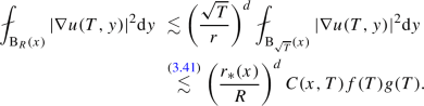
-
(ii)
In the case where \(\sqrt{\frac{T}{2}}\ge 2r_*(x)\), we combine, by noticing that \(\partial _{\tau } u-\nabla \cdot a\nabla u=0\) on \((\frac{T}{2},T)\times \text {B}_{\sqrt{\frac{T}{2}}}(x)\), Lemma 2 and the large-scale \(\text {C}^{0,1}\) estimate (B.4) to obtain

-
(i)
-
2.
We now consider the generic case \(R\ge r_*(x)\) and, without loss of generality, we may assume that \(\sqrt{T}>2\sqrt{2}R\) since otherwise
 and the conclusion follows from (3.41). We have \(\partial _{\tau } u-\nabla \cdot a\nabla u=0\) on \((0,T)\times \text {B}_{\sqrt{T}}\) and \(r_*(x)\le 2R<\sqrt{\frac{T}{2}}\) so that from Lemma 2 and the large-scale \(\text {C}^{0,1}\)estimate (B.4) we deduce


 and the conclusion follows from (
4.3 Proof of the suboptimal control of fluctuations of the time dependent flux
We provide in this section the proofs of Lemmas 6, 7, 8 and Proposition 1 of Sect. 3.4.
4.3.1 Proof of Lemmas 6 and 7: control of the functional derivatives
We prove Lemmas 6 and 7 independently. For heuristic arguments, we refer to I) in Sect. 3.1.
Proof of Lemma 6
It is enough to prove (3.43) for the quantities \(q_r(T)\cdot e_k\), for all \(r>0\), \(T\ge 1\) and \(k\in \llbracket 1,d\rrbracket \). In particular, we only treat the case \(k=1\), since the other contributions are controlled the same way. For notational convenience, we simply write \(v^T\) for \(v^T_1\).
Let \(x\in {\mathbb {R}}^d\), \(h\in (0,1)\), \(T\ge 1\), \(r>0\), \(\ell \in [1,\infty )\) and \(\delta a\) be compactly supported in \(\text {B}_{\ell }(x)\) such that \(\sup _{y\in \text {B}_{\ell }(x)}\vert \delta a(y)\vert \le 1\). We compute the finite difference
where \(\delta ^h u(t,\cdot ):=\frac{u(a+h\delta a,t,\cdot )-u(a,t,\cdot )}{h}\) is the weak solution of
The first r.h.s term of (4.24) gives directly the first r.h.s terms of (3.43). For the second r.h.s term of (4.24), we easily derive from the localized energy estimates (3.33) and (3.34) applied to the equation (4.25) combined with (3.32) with a replaced by \(a+h\delta a\) (which control the norm of the r.h.s of (4.25)) that
We thus obtain the second second r.h.s term of (3.43). We now focus on the third r.h.s term of (4.24). We split the time integral into the singular part \(t\le 1\) and the regular part \(t\ge 1\)
We now split the rest of the proof into two steps, treating the two r.h.s terms of (4.26) separately.
Step 1. First r.h.s term of (4.26). We prove that

where \({\mathcal {T}}_{x,\ell }(\eta _r)\) is defined in (3.47). We argue differently between the two regimes \(\ell <\sqrt{T}\) and \(\ell \ge \sqrt{T}\).
Regime \(\ell <\sqrt{T}\). Using that  and by splitting \({\mathbb {R}}^d\) into \(\text {B}_{\ell }(x)\) and \({\mathbb {R}}^d\backslash \text {B}_{\ell }(x)\), we have

We now show that

Since the arguments are similar we only give the details for \(I^{\ell }_2\). By Cauchy–Schwarz’s inequality, we have

It remains to estimate the first r.h.s factor of (4.30). First, by the localized energy estimate (3.34) applied to the Eq. (4.25) and \(\bigg (\int _{\text {B}_{\ell }(x)}\vert \delta a(y) e\vert ^2\text {d} y\bigg )^{\frac{1}{2}}\lesssim \ell ^{\frac{d}{2}}\), we obtain

Second, by the localized energy estimate (3.32) applied to the equation (2.11) with a replaced by \(a+h\delta a\) and for \(R=\ell \ge 1\), we obtain (since \(\mathbbm {1}_{\text {B}_{\ell }(x)}(y)\lesssim e^{-\frac{\vert y-x\vert }{\ell }}\))
and
Finally the combination of (4.30), (4.31), (4.32) and (4.33) yields (4.29). It then follows from (4.28) that

Regime \(\ell \ge \sqrt{T}\). Using Cauchy–Schwarz’s inequality and by dominating the Gaussian kernel \(g_r\) by the exponential kernel \(\eta _r\), we have
with, by applying the localized energy estimates (3.32) and (3.33) to (4.25) for \(R=r\)
Now, since \(\delta a\) is supported in \(\text {B}_{\ell }(x)\), the localized energy estimates (3.33) and (3.34) applied to the Eq. (4.25) with \(R=\ell \) combined with (4.32) and (4.33) yield
which allow us to pass to the limit when \(h\downarrow 0\) in (4.35) and (4.36), and obtain
This concludes the argument for (4.27).
Step 2. Second r.h.s term of (4.26). We prove that

Recall that \(v^T\) denotes the weak solution of the dual system associated with (4.25), which reads
We reformulate the l.h.s of (4.38) with help of the dual system (4.39). We have by testing the Eq. (4.39) with \(\delta ^h u\) and integrating in time
and also, by testing (4.25) with \(v^T\)
Consequently, by summing (4.40) and (4.41), using an integration by part in time and the fact that \(v^T(T,\cdot )\equiv 0\), we get
Moreover, from (4.37) we can pass to the limit when \(h\downarrow 0\) in the second r.h.s term of (4.42), namely
and obtain the first r.h.s term of (4.38). It remains to control the first r.h.s term of (4.42). To this aim, we integrate in time the Eq. (4.25) between 0 and 1:
which provides by testing with \(v^T(1,\cdot )\)
The first and the third r.h.s terms of (4.43) combined with (4.37) give the second r.h.s term of (4.38). The second r.h.s term of (4.43) is then dominated in two ways, depending on the regime in \(\ell \).
Regime \(\ell \ge \sqrt{T}\). For the generic case \(\ell \ge r_*(0)\), we use the identity  and we split the integral into the two contributions \(\int _{{\mathbb {R}}^d\backslash \text {B}_{4\ell }}\) and \(\int _{\text {B}_{4\ell }}\) in form of

For the far-field contribution \(\vert y\vert \ge 4\ell \), we use of Cauchy–Schwarz’s inequality and the computations done in (4.36) as well as (4.37) to get

For the near-field contribution \(\vert y\vert <4\ell \), we first note that from the assumption \(\ell >r_*(0)\) we have for all \(y\in {\mathbb {R}}^d\)
Indeed, from the \(\frac{1}{8}\)-Lipschitz regularity property of \(r_*\), if there exists \(z\in \text {B}_{r_*(y)}(y)\cap \text {B}_{5\ell }\) then \(\vert y\vert \le \vert y-z\vert +\vert z\vert \le r_*(y)+5\ell \le r_*(0)+\frac{\vert y\vert }{8}+5\ell \le 6\ell +\frac{\vert y\vert }{8}\) and thus \(\vert y\vert \le \frac{16}{3}\ell \le 7\ell \). Therefore, using the property (B.18) combined with Cauchy–Schwarz’s inequality, we get

and we finally end up with, using (4.36) as well as (4.37)

For the non-generic regime \(\ell < r_*(0)\), we use the estimate (4.34) which clearly holds by replacing \(g_r\) with \(v^T(1,\cdot )\) and we bound \(\ell ^{\frac{d}{2}}\) by \(r^{\frac{d}{2}}_*(0)\).
Regime \(\ell <\sqrt{T}\). We use the estimate (4.34) which clearly holds by replacing \(g_r\) with \(v^T(1,\cdot )\). \(\square \)
We now turn to the proof of Lemma 7.
Proof of Lemma 7
We keep the notations of the previous proof and we give only the argument for \(q(r^2)\star f_r\cdot e_1\). First, equality (4.24) holds and take the form
The first two r.h.s terms of (4.45) give directly the first two r.h.s terms of (3.49), respectively. As in (4.26), we make the decomposition
Control of the second r.h.s term of (4.46) This term is controlled the same way as we did in Step 2 of the proof of Lemma 6 and provides the third, the fifth and the sixth r.h.s term of (3.49).
Control of the first r.h.s term of (4.46) It remains to argue that the first r.h.s term of (4.46) is dominated by the fourth r.h.s term of (3.49). We distinguish the two regimes \(\ell \ge r\) and \(\ell \le r\).
Regime \(\ell \ge r\). We use the assumption (3.48) in form of, for all \(y\in {\mathbb {R}}^d\), \(\vert f_r(y)\vert \lesssim \int _{1}^{r^2}s^{-\frac{1}{2}}g_{\sqrt{2s}}(y)\text {d} s\) and (4.36) applied with \(r=\sqrt{s}\) to get
Regime \(\ell < r\). We first note that from the assumption (3.48) we have, for all \(y\in {\mathbb {R}}^d\)
We now make use of the identity  to get

We then split the integral into the far-field contribution \(\vert y\vert \ge 2\ell \) and the near-field contribution \(\vert y\vert <2\ell \). For the near-field contribution, we make use of a dyadic decomposition and (4.47) in form of \(\vert f_r(y)\vert \lesssim (\vert y\vert +1)^{-d+1}\) to get

which gives the first term in the second r.h.s term of (3.51) by passing to the \(\limsup \) and combining (4.36), applied both with \(R=1\) and \(R=2^{n+1}\), with (4.37). For the far-field contribution, we make use of Cauchy–Schwarz’s inequality in form of

and we get the second term in the second r.h.s term of (3.51) by passing to the \(\limsup \) and combining (4.36), applied with \(R=\ell \), with (4.37). \(\square \)
4.3.2 Proof of Lemma 8
We split the proof into two steps. In the first step, we prove a deterministic bound on \(q_r(T,x)\), using the energy estimates of Lemma 1 and the control of averages of \(\nabla u\) deduced from Lemma 5. The deterministic bound will depend on a random variable built from an average of \(r_*\). In the second step, we prove that the random constant has stretched exponential moments, using the moment bound (B.1) on \(r_*\).
Step 1. Proof that for all \(r\le \min \{1,\sqrt{T}\}\) and \(x\in {\mathbb {R}}^d\)
Without loss of generality, we may assume that \(x=0\). We use the definition (2.14) of \(q_r(T)\) followed by the triangle inequality, the domination of the Gaussian kernel \(g_r\) by the exponential kernel \(\eta _r\) and the continuous embedding \(\text {L}^2({\mathbb {R}}^d,\eta _r\text {d} x)\hookrightarrow \text {L}^1({\mathbb {R}}^d,\eta _r \text {d} x)\) to obtain
For the first r.h.s term of (4.49), we use the energy estimate (3.32) in form of
For the second r.h.s term of (4.49), we write with  and Cauchy–Schwarz’s inequality,

Using the energy estimate (3.32) applied to the equation (2.11) in form of, for all \(T>0\)

we deduce from Minkowski’s inequality in \(\text {L}^2(\text {B}_r(x))\) and Lemma 5 applied with \(R=1\), \(f\equiv 1\) and \(g:T\in {\mathbb {R}}^+\mapsto T^{-1}\), that, since \(r\le 1\)

Consequently (4.50) turns into

It remains to show that

For this, we decompose \({\mathbb {R}}^d\) into \(\text {B}_r\) and \({\mathbb {R}}^d\backslash \text {B}_r\) to the effect of

The first r.h.s term of (4.52) is controlled by, using the \(\frac{1}{8}\)-Lipschitz regularity of \(r_*\) in form of \(\sup _{x\in \text {B}_r} r_*(x)\lesssim r_*(0)+r\lesssim r_*(0)+1\) and Cauchy–Schwarz’s inequality

For the second r.h.s term of (4.52), we note that for all \(x\in {\mathbb {R}}^d\backslash \text {B}_r\) and \(y\in \text {B}_r(x)\) we have \(\eta _r(y)\lesssim \eta _r(x)\), so that

This concludes the proof of (4.51) and the argument for (4.48).
Step 2. We prove (3.52). It remains to show that \({\mathcal {C}}_\star (r,x):=1+r^{\frac{d}{2}}_*(0)+\int _{{\mathbb {R}}^d\backslash \text {B}_1(x)}\eta _1(y)r^{\frac{d}{2}}_*(ry+x)\text {d} y\) has the desired stretched exponential moment (3.53). From the moment bound (B.1) of \(r_*\) and the equivalence between algebraic moments and exponential moments (see Lemma 9), we haveFootnote 2 for any \(\gamma >0\)
Therefore,
which gives (3.52) by applying once again Lemma 9.
4.3.3 Proof of Proposition 1: suboptimal fluctuation estimates
We split the proof into three steps. In the first two steps we control \(\int _{{\mathbb {R}}^d}\vert \partial ^{\text {fct}}_{x,\ell }q_r(T)\vert ^2\text {d} x\), using the bound on \(\partial ^{\text {fct}}_{x,\ell }q_r(T)\) proved in Lemma 6, treating separately the two regimes \(\ell <\sqrt{T}\) and \(\ell \ge \sqrt{T}\). In the last step we deduce the desired moment bound (3.42) from the multiscale logarithmic Sobolev inequality, in form of (A.1), and the moment bound (B.1) on \(r_*\). We start with preliminary estimates.
Step 0. Preliminary First, we will use several times the following sub-optimal deterministic decay in time of averages of \(\nabla u\):
This estimate is a direct consequence of the combination of the localized energy estimate (3.32) applied to (2.11) with \(R=\sqrt{t}\) and Lemma 5 applied with \(f\equiv 1\), \(g: t\in {\mathbb {R}}^+\mapsto t^{-2}\) and \(R=\ell \). The estimate (4.54) is our starting point, as the role that (3.5) played in the heuristic arguments of Sect. 3.1.
Second, we will use several times the following large-scale regularity result: for all \(t\in (-\infty ,T]\) and \(x\in {\mathbb {R}}^d\)

where we recall that \(v^T\) is defined in (3.44). This estimate is a consequence of the localized energy estimate (3.32) and the large-scale regularity estimate (3.38). Indeed, we first notice that \(v^{T}=({\tilde{v}}_k(\cdot -T,\cdot ))_{k\in \llbracket 1,d\rrbracket }\) with \({\tilde{v}}_k\) the weak solution of (3.35) for \({\overline{e}}=e_k\) and \(f_r=g_r\). In addition, from the identity (4.4) we get
with \(w=(w_k)_{k\in \llbracket 1,d\rrbracket }\) and \(w_k\) solves (4.5) with \(f_r=g_r\) and \({\overline{e}}=e_k\). Therefore, in the regime \(\sqrt{T-t}\ge 2r_*(x)\), we use (3.38) (where we bound \((\frac{r_*(0)}{r}\vee 1)^{d}\le 2r_*(0)\) since \(r\ge 1\)) in form of

In the regime \(2r_*(x)\ge \sqrt{T-t}\), we use the formula (4.56) combined with the localized energy estimate (3.32) applied with \(R=2r_*(x)\) in form of

Finally the r.h.s is dominated via
with
and
We now turn to the proof of (3.42). In the following, \(p\in [1,\infty )\) denotes an arbitrary stochastic integrability exponent.
Step 1. Regime \(\ell < \sqrt{T}\). Proof that for all \(\ell \in [1,\sqrt{T})\) and \(\gamma <1\)
This estimate corresponds to (3.18) in the heuristic arguments of Sect. 3.1. We split this step into two parts. The first part is devoted to the control of the first four r.h.s terms of (3.43) and the second part is devoted to the control of the last term.
Substep 1.1 Proof that for all \(\ell \in [1,\sqrt{T})\)
and

The estimate of the second l.h.s term of (4.59) corresponds to (3.15) in the heuristic arguments of Sect. 3.1
Argument for (4.58) Since \(r\le \sqrt{T}\), we split \(\int _0^T\) into \(\int _{0}^{r^2}+\int _{r^2}^T\) and we apply the triangle inequality followed by Jensen’s inequality, the identity  as well as Cauchy–Schwarz’s inequality to the effect of
For the first r.h.s term of (4.60), we dominate the Gaussian kernel \(g_r\) by the exponential kernel \(\eta _r\) and we use the localized energy estimate (3.32) applied to (2.11) in form of
For the second r.h.s term of (4.60), since \(\ell <\sqrt{T}\), we have by Minkowski’s inequality in \(\text {L}^2(\text {B}_{\ell }(x))\) and the decay estimate (4.54)
so that we finally get, using in the last line the Lipschitz property of \(r_*\) in form of \(\sup _{y\in \text {B}_{\ell }(x)}\left( \frac{r_*(y)}{\ell }\vee 1\right) ^d\lesssim \left( \frac{r_*(x)}{\ell }\vee 1\right) ^d\) combined with the identity  and change of variables \(x\mapsto \frac{x}{r}\)
Estimate (4.58) then follows in combination with the previous estimate, (4.60) and (4.61) as well as \(\frac{r_*(rx)}{\ell }\vee 1\lesssim r_*(rx)\).
Argument for (4.59) On the one hand, we have from Cauchy–Schwarz’s inequality, the identity  and \(\int _{{\mathbb {R}}^d} g^2_r(y)\text {d} y\lesssim r^{-d}\):
Then, using the localized energy estimate (3.32) applied to (2.11) with \(R=\ell \) and the plain energy estimate \(\int _{{\mathbb {R}}^d}\vert \nabla v^T(1,y)\vert ^2\text {d} y\lesssim r^{-d}\) (the proof is identical as for (4.6)) we get
On the other hand, by noticing that from Fubini–Tonelli’s theorem, we have for all measurable functions \(f : {\mathbb {R}}^d\rightarrow {\mathbb {R}}^+\)

we get, recalling that \(\int _{{\mathbb {R}}^d}\vert \nabla v^{T}(1,y)\vert ^2\text {d} y\lesssim r^{-d}\),

The combination of (4.62), (4.63) and (4.64) give the desired (4.59).
Substep 1.2 Proof that for all \(\ell \in [1,\sqrt{T})\)
For heuristic arguments which lead to (4.65), we refer to (3.17) in Sect. 3.1.
Let \(N:= \left\lceil \log _2(T)\right\rceil \). We start by decomposing the time interval [1, T] into dyadic intervals \([2^j,2^{j+1}]\) for \(j\in \llbracket 1,N-1\rrbracket \). By the triangle inequality, Cauchy–Schwarz’s inequality and the decay estimate (4.54)
In addition, by the \(\frac{1}{8}\)-Lipschitz property of \(r_*\) in form of \(r_*(x)\vee \ell \lesssim \inf _{y\in \text {B}_{\ell }(x)}r_*(y)\vee \ell \) and \(\sup _{y\in \text {B}_{r*(x)}(x)}r_*(y)\vee \ell \lesssim r_*(x)\vee \ell \) as well as the identity  and the property (B.18), we have for all \(j\in \llbracket 0,N-1\rrbracket \)

Then, using the large-scale estimate (4.55) we have

Therefore, from (4.68), (4.69) and the change of variables \(x\mapsto \frac{x}{r}\), we get
which gives the estimate (4.65) by plugging (4.70) into (4.67) and using \(\eta _{4r_*(x)}(x)\lesssim r^d_*(x)(\vert x\vert +1)^{-2d}\) as well as \(\frac{r_*(x)}{\ell }\vee 1\lesssim r_*(x)\). This concludes the argument for the first item of (4.58). Finally, we recall (4.53):
Applying (4.71) directly on the random variables involved in (4.58) and (4.65) yields the second item of (4.58).
Step 2. Regime \(\ell \ge \sqrt{T}\). Proof that for all \(\ell \in [\sqrt{T},\infty )\)
with for any \(\gamma >0\)
This estimate corresponds to (3.26) in the heuristic arguments of Sect. 3.1. We split this step into two parts. The first one is devoted to the control of the first four r.h.s terms of (3.43) and the second one is devoted to the control of the last r.h.s term.
Substep 2.1 Proof that for all \(\ell \in [\sqrt{T},\infty )\)
as well as
where we recall that \({\mathcal {G}}_{r,\ell }\) is defined in (3.46). The estimate of the first l.h.s of (4.75) corresponds to (3.21) in the heuristic arguments of Sect. 3.1.
Argument for (4.74) For the first item, we use Young’s inequality in form of
For the second item, we use for all \(x\in {\mathbb {R}}^d\), \(\int _{\text {B}_{\ell }(x)}g_r(y)\text {d} y\le \int _{{\mathbb {R}}^d}g_r(y)\text {d} y\lesssim 1\), Cauchy–Schwarz’s inequality applied in form of \((\int _{\text {B}_{\ell }(x)}f(y)g_r(y)\text {d} y)^2\le \int _{\text {B}_{\ell }(x)}g_r(y)\text {d} y\int _{\text {B}_{\ell }(x)}\vert f(y)\vert ^2 g_r(y)\text {d} y\) and the identity  , to get
Then, since \(r\le \sqrt{T}\), we split the integral \(\int _{0}^T\) into \(\int _{0}^{r^2}+\int _{r^2}^{T}\) and we use the localized energy estimate (3.32) applied to (2.11) in form of \(\int _{{\mathbb {R}}^d}\left| \int _{0}^{r^2}\nabla u(t,y)\text {d} t\right| ^2g_r(y)\text {d} y\lesssim 1\), to obtain
Finally, using that  and for all \(x\in {\mathbb {R}}^d\backslash \text {B}_r\), \(\sup _{y\in \text {B}_r(x)}g_r(y)\lesssim g_r(x)\), in form of

and Minkowski’s inequality in \(\text {L}^2(\text {B}_r(x))\) as well as the decay estimate (4.54) (where we use that, since \(r\ge 1\), \(\frac{r_*(x)}{r}\vee 1\le r_*(x)\)), we deduce

Finally, applying (4.71) on the random variable involved in (4.77) yields (4.74) with the second item in (4.73).
Argument for (4.75) We start with the first l.h.s term. We distinguish between the generic case \(\ell \ge r_*(0)\) and the non-generic case \(\ell <r_*(0)\).
Regime \(\ell \ge r_*(0)\). We split the integral into the far-field contribution \(\vert x\vert \ge 4\ell \) and the near-field contribution \(\vert x\vert <4\ell \). For the far-field contribution, we write using Cauchy–Schwarz’s inequality, the localized energy estimate (3.32) applied to (2.11) with \(R=\ell \) and \(T=1\), the identity \(\int _{{\mathbb {R}}^d\backslash \text {B}_{4\ell }}\int _{\text {B}_{\ell }(x)}\lesssim \ell ^d \int _{{\mathbb {R}}^d\backslash \text {B}_{3\ell }}\) as well as the property (B.18)


By the \(\frac{1}{8}\)-Lipschitz continuity property of \(r_*\) and the assumption \(r_*(0)\le \ell \) one has \(\text {B}_{r_*(x)}(x)\cap {\mathbb {R}}^d\backslash \text {B}_{3\ell }\ne \emptyset \) \(\Rightarrow \) \(x\in {\mathbb {R}}^d\backslash \text {B}_{\ell }\). Indeed, by contradiction and recalling that \(\ell \ge r_*(0)\), if \(x\in \text {B}_{\ell }\) then \(r_*(x)\le r_*(0)+\frac{\vert x\vert }{8}\le \frac{9}{8}\ell \) so that \(\text {B}_{r_*(x)}(x)\subset \text {B}_{\ell +\frac{9}{8}\ell }\subset \text {B}_{\frac{17}{8}\ell }\) and consequently \(\text {B}_{r_*(x)}(x)\cap {\mathbb {R}}^d\backslash \text {B}_{3\ell }=\emptyset \). Hence,

and the above inequality, with help of (4.55) reduces to


For the near-field contribution \(\vert x\vert <4\ell \), using Minkowski’s inequality in \(\text {L}^2(\text {B}_{4\ell })\), Fubini–Tonnelli’s theorem, the property (B.18) and the assumption \(\ell \ge r_*(0)\) in form of (4.44), we write

Then, from the localized energy estimate (3.32) applied to (2.11) with \(R=r_*(x)\) and \(T=1\), we have

consequently, by Cauchy–Schwarz’s inequality and (4.55), (4.83) turns into


Regime \(\ell <r_*(0)\). We use the estimate (4.59) and we bound one \(\ell ^d\) by \(r^d_*(0)\) and \(r^{-d}\) by 1.
We now turn to the second l.h.s term of (4.75). The first term in the definition (3.46) of \({\mathcal {G}}_{r,\ell }\) is bounded as follows. By definition of \({\mathcal {T}}_{x,\ell }(\eta _r)(0)\), that we recall here
and the localized energy estimates (3.32) as well as (3.33) applied to (2.11), Minkowski’s inequality in \(\text {L}^2({\mathbb {R}}^d)\) (exchanging the order of integration in the s and x variables) and the estimate \(\int _{{\mathbb {R}}^d}\int _{\text {B}_{\ell }(x)}\lesssim \ell ^d\int _{{\mathbb {R}}^d}\), we have
For the other term in (3.46), we can use previous estimates. To this aim, we need preliminary inequalities and we distinguish between the two regimes \(\ell \ge r_*(0)\) and \(\ell <r_*(0)\).
Regime \(\ell \ge r_*(0)\). For the far-field contribution \(\vert x\vert \ge 4\ell \), we make use of Cauchy–Schwarz’s inequality in form of, for all \(x\in {\mathbb {R}}^d\)

Next, we have
Indeed, we first split the integral into two contributions
On the one hand, since from the localized energy estimate (3.32) applied to (2.11) with \(R=\ell \) we have \(\sup _{y\in {\mathbb {R}}^d} {\mathcal {T}}_{x,\ell }(\eta _{\ell })(y)\lesssim 1+\int _{0}^1\frac{-\log (t)}{1-t}\text {d} t\lesssim 1\) (we bound the integral \(\int _{\text {B}_{\ell }(x)}\) by \(\int _{{\mathbb {R}}^d}\) in the definition (3.47) of \({\mathcal {T}}_{x,\ell }(\eta _{\ell })(y)\)), we get
On the other hand, for all \(y\in {\mathbb {R}}^d\backslash \text {B}_{2\ell }(x)\) and \(z\in \text {B}_{\ell }(x)\) we have \(\vert z-y\vert \ge \vert y-x\vert -\ell \ge \frac{\vert y-x\vert }{2}\) and thus \(\eta _{\ell }(z-y)\lesssim \eta _{2\ell }(y-x)\). Therefore, the localized energy estimate (3.32) applied to (2.11) with \(R=\ell \) yields
Consequently,
and this concludes the argument for (4.88). The combination of (4.87), (4.88) and the estimate \(\sup _{y\in {\mathbb {R}}^d}\int _{{\mathbb {R}}^d}{\mathcal {T}}_{x,\ell }(\eta _{\ell })(y)\text {d} x\lesssim \ell ^d\) (which can be proved with the same computation as (4.88) by exchanging the role of x and y) leads to

and we then proceed as we did from (4.78) to conclude. For the near-field contribution, we make use of Minkowski’s inequality in \(\text {L}^2({\mathbb {R}}^d)\) and the estimate \(\sup _{y\in {\mathbb {R}}^d}\int _{{\mathbb {R}}^d}{\mathcal {T}}^2_{x,\ell }(\eta _{r_*(y)})(y)\text {d} x\lesssim \ell ^d\) (obtained the same way as (4.86)) to obtain

and we then proceed as we did from (4.84).
Regime \(\ell <r_*(0)\). In this regime, we use the estimate (4.64).
To conclude, the combination of (4.82) (together with \(\int _{{\mathbb {R}}^d\backslash \text {B}_{\ell }} g^2_{2r}(x)\text {d} x\lesssim \ell ^{-d}\) and \(\eta _{4r_*(x)}(x)\lesssim r^d_*(x)\vert x\vert ^{-2d}\)), (4.85) (together with \(\int _{\text {B}_{7\ell }} g_r(y)\text {d} y \lesssim 1\) and \(\eta ^{\frac{1}{2}}_{4r_*(x)}(x)\lesssim r^{\frac{d}{2}+1}_*(x)(\vert x\vert +1)^{-d-1}\)), (4.59) and (4.64) gives (4.75) with
Applying (4.71) on (4.90) followed by a polar change of coordinates and the change of variable \(\rho \mapsto \frac{\rho }{r}\) yields
We then estimate the integral in the integrand of the r.h.s by
which yields the first item in (4.73).
Substep 2.2 Proof that for \(\ell \in [\sqrt{T}, \infty )\)
where we recall that \({\mathcal {D}}_{\star ,1}(r,\ell )\) is defined in (4.90) and satisfies the first item of (4.73). For heuristic arguments which lead to (4.91), we refer to (3.25) in Sect. 3.1.
For the proof of (4.91), we argue as previously and we distinguish between the generic case \(\ell \ge r_*(0)\) and the non-generic case \(\ell <r_*(0)\). We mainly make use of previous ideas and estimates.
Regime \(\ell \ge r_*(0)\). As in Substep 1.2, we decompose the time interval [1, T] into dyadic intervals \([2^{j},2^{j+1}]\) for \(j\in \llbracket 1,N-1\rrbracket \) and \(N:=\left\lceil \log _2(T)\right\rceil \) and we write by the triangle inequality
We split the integral in the r.h.s of (4.92) into the far-field contribution \(\vert x\vert \ge 4\ell \) and the near-field contribution \(\vert x\vert < 4\ell \). For the far-field contribution, we write for all \(j\in \llbracket 1,N-1\rrbracket \), using Cauchy–Schwarz’s inequality, the decay estimate (4.54) applied for \(\ell \ge \sqrt{T}\),
We then argue as from (4.78) to (4.79), (4.80), (4.81) and (4.82) (noticing that the evaluation at time 1 plays no role in the estimates) and finally obtain
and we conclude by summing over \(j\in \llbracket 1,N-1\rrbracket \), which gives (4.91) for \(\vert x\vert \ge 4\ell \). For the near-field contribution \(\vert x\vert \le 4\ell \) we write, using Minkowski’s inequality in \(\text {L}^2(\text {B}_{4\ell })\), Fubini–Tonnelli’s theorem, the property (B.18) and the assumption \(\ell \ge r_*(0)\) in form of (4.44)

Then, from the decay (4.54), we have

Thus, by Cauchy–Schwarz’s inequality and (4.69), (4.93) turns into

and we deduce (4.91) for \(\vert x\vert \le 4\ell \), since \(\int _{\text {B}_{7\ell }} g_{2r}(x)\text {d} x\lesssim 1\), \(\eta ^{\frac{1}{2}}_{4r_*(x)}(x)\lesssim r^{\frac{d}{2}+1}_*(x)(\vert x\vert +1)^{-d-1}\) and by summing over \(j\in \llbracket 0, N-1\rrbracket \).
Regime \(\ell <r_*(0)\). We use the estimate (4.65) which holds for \(\ell \ge \sqrt{T}\) by removing \(r^d_*(rx)\) and \(r^d_*(x)\) in each integral in the r.h.s (by using (4.54) for \(\ell \ge \sqrt{T}\)) and we estimate \(\ell ^d\) by \(r^d_*(0)\) as well as \(r^{-\frac{d}{2}}\) by 1.
Step 3. Proof of (3.42) and conclusion We have from the multiscale logarithmic Sobolev inequality in form of (A.1):
We follow the heuristic arguments done in (3.19) and (3.27) of the Sect. 3.1. We split the integral over \(\ell \) into two parts.
-
(i)
In the regime \(\ell <\sqrt{T}\) we use (4.58):
$$\begin{aligned}&\left\langle \left( \int _{1}^{\sqrt{T}}\ell ^{-d} \pi (\ell )\int _{{\mathbb {R}}^d}\vert \partial ^{\text {fct}}_{x,\ell } q_r(T)\vert ^2\text {d} x\, \text {d} \ell \right) ^{\frac{p}{2}}\right\rangle ^{\frac{1}{p}}\nonumber \\&\quad {\mathop {\lesssim }\limits ^{(4.57)}}r^{-\frac{d}{2}}(1+\log (T)+\log (\tfrac{\sqrt{T}}{r}))\left\langle \left( \int _{1}^{\sqrt{T}}\ell ^d \pi (\ell ){\mathcal {C}}_\star (r,\ell )\text {d} \ell \right) ^{\frac{p}{2}}\right\rangle ^{\frac{1}{p}}\nonumber \\&\quad {\mathop {\le }\limits ^{(2.6)}}r^{-\frac{d}{2}}(1+\log (T)+\log (\tfrac{\sqrt{T}}{r}))\left( \int _{1}^{\sqrt{T}}\ell ^{d-1-\beta }\left\langle {\mathcal {C}}^{p}_\star (r,\ell )\right\rangle ^{\frac{1}{p}}\text {d} \ell \right) ^{\frac{1}{2}}\nonumber \\&\quad {\mathop {\lesssim _\gamma }\limits ^{(4.57)}} (p^{\frac{d}{\beta \wedge d}}\mathbbm {1}_{\beta \ne d}+p^{1+\gamma }\mathbbm {1}_{\beta =d})\,r^{-\frac{d}{2}}(1+\log (T)+\log (\tfrac{\sqrt{T}}{r}))\mu _{\beta }(T), \end{aligned}$$(4.96)by the definition (2.19) of \(\mu _{\beta }(T)\).
-
(ii)
In the regime \(\ell \ge \sqrt{T}\) we use (4.71), (4.72), (4.73) and the change of variable \(\ell \mapsto \frac{\ell }{\sqrt{T}}\) and the fact that \(r\le \sqrt{T}\) in the last line:
$$\begin{aligned}&\left\langle \left( \int _{\sqrt{T}}^{+\infty }\ell ^{-d} \pi (\ell )\int _{{\mathbb {R}}^d}\vert \partial ^{\text {fct}}_{x,\ell } q_r(T)\vert ^2\text {d} x\, \text {d} \ell \right) ^{\frac{p}{2}}\right\rangle ^{\frac{1}{p}}\nonumber \\&\quad {\mathop {\lesssim }\limits ^{(4.72),(2.6)}}\log (T)\left\langle \left( \int _{\sqrt{T}}^{+\infty }\ell ^{-1-\beta }(r^{2d}_*(0)+{\mathcal {D}}_{\star ,1}(r,\ell ))\text {d} \ell \right) ^{\frac{p}{2}}\right\rangle ^{\frac{1}{p}}\nonumber \\&\qquad +\log (\tfrac{\sqrt{T}}{r})\left\langle {\mathcal {D}}^{\frac{p}{2}}_{\star ,2}(r)\right\rangle ^{\frac{1}{p}}\left( \int _{\sqrt{T}}^{+\infty } \ell ^{-1-\beta }\text {d} \ell \right) ^{\frac{1}{2}}\nonumber \\&\quad \lesssim T^{-\frac{\beta }{4}}\log (T)\left( \int _{1}^{+\infty }\ell ^{-1-\beta }\left\langle (r^d_*(0)+{\mathcal {D}}_{\star ,1}(r,\ell \sqrt{T}))^p\right\rangle ^{\frac{1}{p}}\text {d} \ell \right) ^{\frac{1}{2}}\nonumber \\&\qquad +\log (\tfrac{\sqrt{T}}{r})\left\langle {\mathcal {D}}^{\frac{p}{2}}_{\star ,2}(r)\right\rangle ^{\frac{1}{p}}\nonumber \\&\quad {\mathop {\lesssim _\gamma }\limits ^{(4.73), (4.71)}} r^{-\frac{d}{2}}\mu _{\beta }(T)\Big ((p^{\frac{d+1}{\beta \wedge d}}\mathbbm {1}_{\beta \!\ne \! d}\!+\!p^{(1+\frac{1}{d})(1+\gamma )}\mathbbm {1}_{\beta =d})\log (T)(1\!+\!\log ^2(\tfrac{\sqrt{T}}{r}))\nonumber \\&\qquad +(p^{\frac{d}{\beta \wedge d}}\mathbbm {1}_{\beta \ne d}+p^{1+\gamma }\mathbbm {1}_{\beta =d})\log (\tfrac{\sqrt{T}}{r})\Big ). \end{aligned}$$(4.97)
The combination of (4.96) and (4.97) gives the desired bound (3.42).
4.4 Proof of the main results
4.4.1 Proof of Theorem 1: fluctuations of the time dependent flux
We only give the argument for the flux q(T), the computations for \(\phi (T)\) are done by a straightforward adaptation of the argument of this proof and the ones to prove Lemmas 6 and 7.
Our first goal is to remove the \(\log (T)\) correction in the r.h.s of (3.42), which will lead to (2.18). To this aim, we first use the \(\text {L}^2{-}\text {L}^1\) type estimate of Lemma 3, which allow us to make the link between the \(r^{-\frac{d}{2}}\) decay of the fluctuations of \((q_r(T,\cdot ))_{r\le \sqrt{T}}\) proved in Proposition 1 and the decay in T of moments of \((\int _{{\mathbb {R}}^d}\eta _R\vert \nabla u(T,\cdot )\vert ^2)_{R\ge \sqrt{T}}\). This yields an improvement on the decay in T, see (4.98). With this new decay in hand, we are able to obtain optimal estimates in scaling. The price to pay in this step is a small loss of stochastic integrability. Our second goal is to prove estimate (2.21). This does not require new ideas and this is done by dominating carefully the terms in the derivative (3.49) and by using some estimates already established in the proof of (2.18).
Proof of (2.18)
We split the proof into three steps. In the following, \(p\in [1,\infty )\) denotes an arbitrary stochastic integrability exponent.
Step 1. Improvement of (4.54) Proof that for all \(x\in {\mathbb {R}}^d\), \(T\ge 1\) and \(\varepsilon \in (0,1)\)
with
and for some stationary random field \({\mathcal {D}}_\star (T,\ell ,\cdot )\) that satisfies for any \(\gamma >0\)
where \(\alpha _\gamma \) as in Proposition 1. We have from Lemma 3, Minkowski’s inequality in \(\text {L}^p_{\left\langle \cdot \right\rangle }(\Omega )\) and the stationarity of \(q_r\): for all \(T\ge 4\) and \(R\ge \sqrt{T}\)

Then, we split the integral over \([0,\sqrt{t}]\) into the two contributions \(r\le 1\) and \(1\le r\le \sqrt{t}\):
-
(i)
For \(r\le 1\) we use (3.52) and the change of variable \(r\mapsto \tfrac{\sqrt{T}}{r}\):
 (4.102)
 -
(ii)
For \(1\le r\le \sqrt{t}\) we use (3.42) and the change of variable \(r\mapsto \tfrac{\sqrt{T}}{r}\):
 (4.103)
where \(\eta _{\beta }\) is defined in (2.25).


The combination of (4.101), (4.102) and (4.103) yields that for all \(x\in {\mathbb {R}}^d\) and \(R\ge \sqrt{T}\)

where  has the moment bound (4.100). This implies, from Lemma 5 applied with \(f: t\in {\mathbb {R}}_*^+\mapsto \log ^2(t)\) and \(g:t\in {\mathbb {R}}_*^+\mapsto t^{-2-\frac{d}{2}}\) that, for all \(\ell <\sqrt{T}\)

By interpolating between (4.54) and the combination of (4.104) and (4.105) as well as using that \(\frac{r_*(x)}{\ell }\vee 1\le 2r_*(x)\) in the last line, we finally obtain for all \(\varepsilon \in (0,1)\)
with \(\eta _{\varepsilon , \beta }\) defined in (4.99) and  which satisfies the moment bound (4.100).
Step 2. Equipped with (4.98), we improve the estimates (4.58) and (4.72) for the control of \((x,\ell )\mapsto \int _{{\mathbb {R}}^d}\vert \partial ^{\text {fct}}_{x,\ell } q_r(T)\vert ^2\text {d} x\) (corresponding to the substeps 1 and 2 of the proof of Lemma 1). We split this step into two parts, one for the improvement of (4.58) and an other for (4.72), treating separately the two regimes \(\ell <\sqrt{T}\) and \(\ell \ge \sqrt{T}\).
Substep 2.1 Improvement of (4.58). Proof that for all \(\varepsilon >0\) and \(\ell <\sqrt{T}\)
where

and
The estimate (4.59) is unchanged and gives the first contribution in (4.106). We improve the estimates (4.58) and (4.65) (corresponding to the estimate of the second and last r.h.s term of (3.43), respectively). On the one hand, noticing that from Minkwoski’s inequality in \(\text {L}^2({\mathbb {R}}^d)\) and (4.98) as well as \(r\ge \frac{1}{2}\), we have for all \(x\in {\mathbb {R}}^d\)
thus we deduce from (4.60) and (4.61) that
where
Using the change of variables \(x\mapsto \frac{x}{r}\) in the last r.h.s term of (4.109), this gives the term \({\mathcal {E}}_{\star ,\varepsilon }(r,\ell )\) defined in (4.107). On the other hand, noticing that, by monotonicity of \(t\in {\mathbb {R}}^+_*\mapsto \eta _{\varepsilon ,\beta }(t)\), for all \(j\in {\mathbb {N}}\), we have
we deduce from (4.66) and (4.98)
It remains to control the r.h.s integral of (4.111) by \(2^{j}r^{-d}{\mathcal {F}}_{j,\star ,\varepsilon }(r,\ell )\), where \({\mathcal {F}}_{j,\star ,\varepsilon }(r,\ell )\) is defined in (4.108). To this aim, we note that, by the \(\frac{1}{8}\)-Lipschitz property of \(r_*\), we have for all \((x,y)\in {\mathbb {R}}^{2d}\)
Indeed if there exists \(z\in \text {B}_{\ell }(x)\cap \text {B}_{r_*(y)}(y)\), we have by the triangle inequality
and thus (4.112) holds. Then, we use the property (B.18) and the decomposition, for all \(x\in {\mathbb {R}}^d\), \(\int _{{\mathbb {R}}^d}=\int _{\text {B}_{\ell }(x)}+\int _{{\mathbb {R}}^d\backslash \text {B}_{\ell }(x)}\), to obtain

Next, we make use of (4.112) to bound the second r.h.s term of (4.113) with

The combination of (4.113) and (4.114) (where we bound \((r_*(x)\vee \ell )^{d+\varepsilon }\lesssim \ell ^{d+\varepsilon }r^{d+\varepsilon }_*(x)\)) as well as (4.69) (where we bound \(\eta _{4r_*(x)}(x)\lesssim r^d_*(x)(\vert x\vert +1)^{-2d}\)) proves that the r.h.s integral of (4.111) is indeed bounded by \(2^j r^{-d}{\mathcal {F}}_{j,\star ,\varepsilon }(r,\ell )\) and this concludes the argument for (4.106).
Substep 2.2 Improvement of (4.72). Proof that for all \(\varepsilon >0\) and \(\ell \ge \sqrt{T}\)
with \({\mathcal {D}}_{\star ,1}(r,\ell )\) and \({\mathcal {D}}_{\star ,2}(r)\) as in (4.73),
as well as for all open subsets \({\mathcal {U}}\) of \({\mathbb {R}}^d\)
The estimates (4.74) and (4.75) are unchanged and give respectively the \(\ell ^d{\mathcal {D}}_{\star ,2}(r)\log ^2(\tfrac{\sqrt{T}}{r})\) and \(\ell ^d{\mathcal {D}}_{\star ,1}(r,\ell )\) contributions in the r.h.s of (4.115). We improve the estimate (4.91). We argue differently between the generic case \(\ell \ge r_*(0)\) and the non-generic case \(\ell <r_*(0)\).
Regime \(\ell \ge r_*(0)\). We have from (4.92)
We then split the argument between the far-field regime \(\vert x\vert \ge 4\ell \) and the near-field regime \(\vert x\vert \le 4\ell \). For the far-field regime, we use Cauchy–Schwarz’s inequality combined with (4.98) (applied for \(\ell \ge \sqrt{T}\)) and (4.110) to the effect of
This then gives the first term of (4.116) by dominating \(\int _{2^{j}}^{2^{j+1}}\int _{\text {B}_{\ell }(x)}\vert \nabla v^T(t,y)\vert ^2\text {d} y\, \text {d} t\) using the arguments for (4.113) and (4.114). For the near-field regime, we use (4.98) and (4.110) in form of

which has the effect of, combined with (4.93) and Cauchy–Schwarz’s inequality

and yields the third term of (4.116) by using (4.69) (where we use \(\eta _{4r_*(x)}(x)\lesssim r^d_*(x)(\vert x\vert +1)^{-2d}\)).
Regime \(\ell <r_*(0)\). For the non-generic case \(\ell <r_*(0)\), we use (4.111), (4.113), (4.114) and we bound one \(\ell ^d\) by \(r^d_*(0)\) which gives the second term of (4.116).
Step 3. Proof of (2.23). We have from the multiscale logarithmic Sobolev inequality in form of (A.1), for all \(p\in [1,\infty )\)
with
We then treat separately the two terms above.
-
(i)
In the regime \(\ell <\sqrt{T}\) we use (4.106) combined with Minkowski’s inequality in \(\text {L}^p_{\left\langle \cdot \right\rangle }(\Omega )\):
$$\begin{aligned} {\mathcal {I}}^1_{\sqrt{T}}&{\mathop {\lesssim }\limits ^{(4.106)}} r^{-\frac{d}{2}}\left\langle \bigg (\int _{1}^{\sqrt{T}}\ell ^d\pi (\ell )\bigg (1+{\mathcal {E}}_{\star ,\varepsilon }(r,\ell )+\Big (\sum _{j=0}^{+\infty }2^{\frac{j}{2}}\eta _{\varepsilon ,\beta }(2^j){\mathcal {F}}_{j,\star ,\varepsilon }(r,\ell )\Big )^2\bigg )\text {d} \ell \bigg )^{\frac{p}{2}}\right\rangle ^{\frac{1}{p}}\nonumber \\&{\mathop {\le }\limits ^{(2.6)}}r^{-\frac{d}{2}}\bigg (\int _{1}^{\sqrt{T}}\ell ^{d-1-\beta }\bigg (1+\left\langle {\mathcal {E}}^p_{\star ,\varepsilon }(r,\ell )\right\rangle ^{\frac{1}{p}}\nonumber \\&\qquad +\Big (\sum _{j=0}^{+\infty }2^{\frac{j}{2}}\eta _{\varepsilon ,\beta }(2^j)\left\langle {\mathcal {F}}^{2p}_{j,\star ,\varepsilon }(r,\ell )\right\rangle ^{\frac{1}{2p}}\Big )^2\bigg )\text {d}\ell \bigg )^{\frac{1}{2}}\nonumber \\&\lesssim r^{-\frac{d}{2}}\mu _{\beta }(T)\bigg (1+\sup _{\ell \ge 1}\left\langle {\mathcal {E}}^p_{\star ,\varepsilon }(r,\ell )\right\rangle ^{\frac{1}{2p}}+\sup _{\ell \ge 1}\sum _{j=0}^{+\infty }2^{\frac{j}{2}}\eta _{\varepsilon ,\beta }(2^j)\left\langle {\mathcal {F}}^{2p}_{j,\star ,\varepsilon }(r,\ell )\right\rangle ^{\frac{1}{2p}}\bigg ), \end{aligned}$$(4.121)by the definition (2.19) of \(\mu _{\beta }\).
-
(ii)
In the regime \(\ell \ge \sqrt{T}\) we use (4.115), Minkowski’s inequality in \(\text {L}^p_{\left\langle \cdot \right\rangle }(\Omega )\) and the fact that \(r\le \sqrt{T}\) in the last line:
$$\begin{aligned} {\mathcal {I}}^2_{\sqrt{T}}\lesssim&\left\langle \bigg (\int _{\sqrt{T}}^{+\infty }\pi (\ell )\bigg ({\mathcal {D}}_{\star ,1}(r,\ell )+{\mathcal {D}}_{\star ,2}(r)\log ^2(\tfrac{\sqrt{T}}{r})\right. \nonumber \\&\left. +\Big (\sum _{j=0}^{+\infty } 2^{\frac{j}{2}}\eta _{\varepsilon ,\beta }(2^j){\mathcal {H}}_{j,\star ,\varepsilon }(r,\ell )\Big )^2\bigg )\text {d}\ell \bigg )^{\frac{p}{2}}\right\rangle ^{\frac{1}{p}}\nonumber \\ {\mathop {\lesssim }\limits ^{(2.6)}}&\bigg (\int _{\sqrt{T}}^{+\infty }\ell ^{-1-\beta }\bigg (\left\langle {\mathcal {D}}^{p}_{\star ,1}(r,\ell )\right\rangle ^{\frac{1}{p}}+\left\langle {\mathcal {D}}^{p}_{\star ,2}(r)\right\rangle ^{\frac{1}{p}}\log ^{2}(\tfrac{\sqrt{T}}{r})\nonumber \\&+\Big (\sum _{j=0}^{+\infty }2^{\frac{j}{2}}\eta _{\varepsilon ,\beta }(2^j)\left\langle {\mathcal {H}}^{2p}_{j,\star ,\varepsilon }(r,\ell )\right\rangle ^{\frac{1}{2p}}\Big )^2\bigg )\text {d}\ell \bigg )^{\frac{1}{2}}\nonumber \\ \lesssim&\, r^{-\frac{d}{2}}\mu _{\beta }(T)\bigg (\Big (\int _{1}^{+\infty }\ell ^{-1-\beta }\left\langle {\mathcal {D}}^{p}_{\star ,1}(r,\ell \sqrt{T}))\right\rangle ^{\frac{1}{p}}\text {d} \ell \Big )^{\frac{1}{2}}\nonumber \\&+\log (\tfrac{\sqrt{T}}{r})\sup _{r\ge 1}\left\langle {\mathcal {D}}^{p}_{\star ,2}(r)\right\rangle ^{\frac{1}{2p}}\nonumber \\&+\sup _{\ell \ge 1}\sum _{j=0}^{+\infty }2^{\frac{j}{2}}\eta _{\varepsilon ,\beta }(2^j)\left\langle {\mathcal {H}}^{2p}_{j,\star ,\varepsilon }(r,\ell )\right\rangle ^{\frac{1}{2p}}\bigg ). \end{aligned}$$(4.122)
It remains to show that, for all \(\varepsilon \in (0,1)\)
and
This is a direct consequence of the combination of (4.100), (4.71) and \(\sum _{j=0}^{+\infty }2^j\eta _{\varepsilon ,\beta }(2^j)\lesssim _{\varepsilon } 1\). \(\square \)
We now turn to the proof of (2.21). The proof does not require new ideas and essentially uses estimates previously established.
Proof of (2.21)
We use the same notations as in the previous proof. We split the proof into two parts, treating separately the two regimes \(\ell < r\) and \(\ell \ge r\). We start with preliminary estimates.
Step 0. Preliminary First, we will use several times the assumption (2.20) in form of (4.47), that we restate here:
Second, we note that from (4.125), we have
and
Therefore, by arguing the same way as for (4.55), using the system (3.50) and the estimate (3.39) instead of (3.38) (since from (4.125), (3.37) holds) as well as the estimate (4.126), we have the following large-scale regularity estimate: for all \(t\in (-\infty ,r^2)\) and \(x\in {\mathbb {R}}^d\)

Step 1. Regime \(\ell <r\). Proof that for all \(\varepsilon >0\) and \(\ell <r\)
with
where for all \(\rho >0\), \({\mathcal {N}}_{\star ,\varepsilon }(r,\ell ,\rho )=r^{d}_*(0)\left( \int _{1}^{r^2}{\mathcal {D}}^{\varepsilon }_{\star }(t,\rho ,0)\eta _{\varepsilon ,\beta }(t)\text {d} t\right) ^2\) (where \({\mathcal {D}}_{\star }\) has the moment bound (4.100)) and
as well as
with for all open set \({\mathcal {U}}\) of \({\mathbb {R}}^d\)
We split this step into two parts. The first part is devoted to the control of the first five r.h.s terms of (3.49).
Substep 1.1 Proof that for all \(\ell \in [1,r)\)
and

as well as
Proof of (4.133). We only give the argument for the second l.h.s term, the first one is dominated the same way. We split the argument into the far-field regime \(\vert x\vert \ge 4\ell \) and the near-field regime \(\vert x\vert <4\ell \). For the near-field regime, we make use of a dyadic decomposition and the estimate (4.125) in form of \(\vert f_r(y)\vert \lesssim (\vert y\vert +1)^{-d+1}\) to get

which gives the second and third r.h.s terms of (4.130) by applying the localized energy estimate (3.32) to the equation (2.11) and the estimate (4.98) (applied for both \(\ell =1\) and \(\ell =2^{n+1}\)) in form of
and for all \(n\in {\mathbb {N}}\)

For the far-field contribution, we first make use of Jensen’s inequality combined with the inequality \(\int _{{\mathbb {R}}^d\backslash \text {B}_{2\ell }}\int _{\text {B}_{\ell }(x)}\text {d} x\lesssim \ell ^d\int _{{\mathbb {R}}^d\backslash \text {B}_{\ell }}\) and the decomposition \(\int _{{\mathbb {R}}^d\backslash \text {B}_{\ell }}=\int _{\text {B}_r\backslash \text {B}_{\ell }}+\int _{{\mathbb {R}}^d\backslash \text {B}_r}\) to obtain
For the first r.h.s term of (4.137), we make use of a dyadic decomposition and the estimate (4.125) in form of \(\vert f_r(y)\vert \lesssim (\vert y\vert +1)^{-d+1}\) to get

which gives the fourth r.h.s term of (4.130) using (4.136). For the second r.h.s term of (4.137), we make use of a dyadic decomposition and (4.125) in form of \(\vert f_r(y)\vert \lesssim r(\vert y\vert +1)^{-d}\) to get

which finally gives fifth r.h.s of (4.130) using once more (4.136).
Proof of (4.134). The estimate of the first two l.h.s terms is an immediate consequence of Minkowski’s inequality in \(\text {L}^2({\mathbb {R}}^d)\) and the estimate (4.86) applied with \(r=\sqrt{s}\), which provides the first r.h.s contribution in (4.134). For the third l.h.s term, we can use previous estimates. To this aim, we use Cauchy–Schwarz’s inequality and (4.88) as well as \(\int _{{\mathbb {R}}^d}{\mathcal {T}}_{x,\ell }(\eta _{\ell })(y)\text {d} x\lesssim \ell ^{d}\) (which may be obtained by changing the role of x and y in the proof of (4.88)) combined with the inequality  to obtain

We then get (4.134) using (4.125) in form of
Proof of (4.135). We start with the first l.h.s term. We distinguish between the generic case \(\ell \ge r_*(0)\) and the non-generic case \(\ell <r_*(0)\).
Regime \(\ell \ge r_*(0)\). We split the integral into the far-field contribution \(\vert x\vert \ge 4\ell \) and the near-field contribution \(\vert x\vert <4\ell \). For the far-field contribution, we make use of the estimates (4.81) (applied with \(T=r^2\)) combined with (4.128) to obtain
which gives the first term in (4.131) using that \(\eta _{4r_*(x)}(x)\lesssim r^d_*(x)(\vert x\vert +1)^{-2d}\). For the near-field contribution, we make use of the estimate (4.84) combined with (4.128) to obtain
which gives the second term of (4.131) using that \(\eta ^{\frac{1}{2}}_{4r_*(x)}(x)\lesssim r^{\frac{d}{2}+1}_*(x)(\vert x\vert +1)^{-d-1}\).
Regime \(\ell <r_*(0)\). We use Cauchy–Schwarz’s inequality, the identity  and the localized energy estimate (3.32) to get
and we conclude with the plain energy estimate in the equation (3.50) (for which a proof is identical as the one for (4.6)) combined with (4.130) that
which gives the first contribution in (4.129). For the second l.h.s term of (4.135), we argue as in (4.87) and (4.89).
Substep 1.2 Proof that for all \(\ell \in [1,r)\)
We argue differently with the generic case \(\ell \ge r_*(0)\) and the non-generic case \(\ell <r_*(0)\) and we use several previous estimates.
Regime \(\ell \ge r_*(0)\). We split the argument between the far-field regime \(\vert x\vert \ge 4\ell \) and the near-field regime \(\vert x\vert <4\ell \). For the far-field contribution, we make use of (4.92), (4.117) and (4.113) as well as (4.114) combined with (4.128) to obtain
For the near-field contribution, we make use of (4.119) combined with (4.128) which leads to
where we used that \(\sum _{j=0}^{+\infty }2^{\frac{j}{2}}\eta _{\varepsilon ,\beta }(2^j)<+\infty \).
Regime \(\ell <r_*(0)\). We make use of (4.111), (4.113) and (4.114) combined with (4.128) and we bound one \(\ell ^d\) by \(r^d_*(0)\) to obtain
Step 2. Regime \(\ell \ge r\). Proof that for all \(\varepsilon >0\) and \(\ell \ge r\)
with

The estimates (4.135) and (4.139) are unchanged. We provide the arguments for the first two and the fourth r.h.s terms of (3.49) and we prove that
and
First, (4.141) follows from Minkowski’s inequality in \(\text {L}^2({\mathbb {R}}^d)\) and (4.86) applied with \(r=\sqrt{s}\) (noticing that the evaluation at 0 plays no role in the estimate). Secondly, using Minkowski’s inequality in \(\text {L}^2({\mathbb {R}}^d)\) and the assumption (2.20), we have
which gives (4.142) using that \(\vert y\vert g_{\sqrt{s}}(y)\lesssim s^{\frac{1}{2}}g_{\sqrt{2s}}(y)\), the estimates (4.76) and (4.77) with (T, r) replaced by \((r^2,s)\)

Step 3. Proof of (2.21). We have from the logarithm Sobolev inequality in form of (A.1), for all \(p\in [1,\infty )\)
with
We then treat separately the two terms above.
-
(i)
In the regime \(\ell <r\) we use (4.129) combined with Minkowski’s inequality in \(\text {L}^p_{\left\langle \cdot \right\rangle }(\Omega )\) and the moment bound (4.71) of \(r_*\) (for \(\gamma =\varepsilon \)) as well as \(\left( \int _{1}^{r}\ell ^{1-\beta }(1+\log (\frac{r}{\ell }+1)\mathbbm {1}_{d=2})\text {d} \ell \right) ^{\frac{1}{2}}\lesssim \chi _{d,\beta }(r)\) and \(1+\log (r+1)\mathbbm {1}_{d=2}\le \chi _{d,\beta }(r)\) (where we recall that \(\chi _{d,\beta }(r)\) is defined in (2.22)):
$$\begin{aligned} {\mathcal {I}}^1_r&\le \bigg \langle \bigg (\int _{1}^r \ell ^{-1-\beta }\bigg (r^d_*(0)(1+\log ^2(r+1)\mathbbm {1}_{d=2})+\ell ^2(1+\log (\frac{r}{\ell }+1)\mathbbm {1}_{d=2})\\&\quad +{\mathcal {M}}_{\star ,1}(r,\ell )+{\mathcal {M}}_{\star ,2}(r,\ell )+\Big (\sum _{j=0}^{+\infty }2^{\frac{j}{2}}\eta _{\varepsilon ,\beta }(2^j){\mathcal {K}}_{j,\star ,\varepsilon }(r,\ell )\Big )^2\bigg )\bigg )^{\frac{p}{2}}\bigg \rangle ^{\frac{1}{p}}\\&\lesssim p^{\frac{d}{\beta \wedge d}+\varepsilon }(1+\chi _{d,\beta }(r))+\bigg (\int _{1}^r\ell ^{-1-\beta }\bigg (\left\langle {\mathcal {M}}^p_{\star ,1}(r,\ell )\right\rangle ^{\frac{1}{p}}+\left\langle {\mathcal {M}}^p_{\star ,2}(r,\ell )\right\rangle ^{\frac{1}{p}}\\&+\sum _{j=0}^{+\infty } 2^{\frac{j}{2}}\eta _{\varepsilon ,\beta }(2^j)\left\langle {\mathcal {K}}^p_{j,\star ,\varepsilon }(r,\ell )\right\rangle ^{\frac{1}{p}}\bigg )\text {d} \ell \bigg )^{\frac{1}{2}}. \end{aligned}$$ -
(ii)
In the regime \(\ell \ge r\) we use (4.140) combined with the Minkowski inequality \(\text {L}^p_{\left\langle \cdot \right\rangle }(\Omega )\):
$$\begin{aligned} {\mathcal {I}}^2_r&\le \big \langle \bigg (\int _{r}^{+\infty }\ell ^{-1-\beta }\bigg (r^2+{\mathcal {M}}_{\star ,3}(r)+{\mathcal {M}}_{\star ,2}(r,\ell )\\&\quad \left. +\Big (\sum _{j=0}^{+\infty } 2^{\frac{j}{2}}\eta _{\varepsilon ,\beta }(2^j){\mathcal {K}}_{j,\star ,\varepsilon }(r,\ell )\Big )^2\bigg )\text {d} \ell \bigg )^{\frac{p}{2}}\right\rangle ^{\frac{1}{p}}\\&\lesssim r^{1-\frac{\beta }{2}}+\bigg (\int _{r}^{+\infty }\ell ^{-1-\beta }\bigg (\left\langle {\mathcal {M}}^p_{\star ,3}(r,\ell )\right\rangle ^{\frac{1}{p}} +\left\langle {\mathcal {M}}^p_{\star ,2}(r,\ell )\right\rangle ^{\frac{1}{p}}\\&\quad +\sum _{j=0}^{+\infty }2^{\frac{j}{2}}\eta _{\varepsilon ,\beta }(2^{j})\left\langle {\mathcal {K}}^p_{j,\star ,\varepsilon }(r,\ell )\right\rangle ^{\frac{1}{p}}\bigg )\text {d} \ell \bigg )^{\frac{1}{2}}. \end{aligned}$$
It remains to prove that for all \(\varepsilon \in (0,1)\)
and
We start with (4.144). First, using the moment bound (4.100) of \({\mathcal {D}}_{\star }\) and the definition of \(\eta _{\varepsilon ,\beta }\) in (4.99) as well as (4.71) (choosing \(\gamma =\varepsilon \)), we have for all \(\rho >0\), \(\left\langle {\mathcal {N}}^p_{\star ,\varepsilon }(r,\ell ,\rho )\right\rangle ^{\frac{1}{p}}\lesssim p^{\frac{d}{\beta \wedge d}+\varepsilon (\alpha _1+\frac{d}{\beta \wedge d})}\). Therefore, by making use of the triangle inequality, we get
Secondly, from the triangle inequality, the moment bounds (4.71) (again for \(\gamma =\varepsilon \)) on \(r_*\) and by splitting the first integral in the r.h.s of (4.131) in form of \(\int _{{\mathbb {R}}^d\backslash \text {B}_{\ell }}=\int _{\text {B}_{r}\backslash \text {B}_{\ell }}+\int _{{\mathbb {R}}^d\backslash \text {B}_{r}}\) as well as (4.138) and (4.127), we have for all \(\ell <r\)
which provides
Finally, using the same decomposition as before and in addition the moment bound (4.100) of \({\mathcal {D}}_{\star }\) we get (up to adjusting \(\varepsilon \))
which concludes the proof of (4.144). We now turn to the proof of (4.145). First, using the moment bound (4.71) (for \(\gamma =\varepsilon \)) on \(r_*\) we have
Secondly, using the triangle inequality
We then argue differently, depending on the regime of \(\beta \) and d:
-
(i)
For \(\beta >2\), we use
$$\begin{aligned}&\int _{{\mathbb {R}}^d\backslash \text {B}_{\ell }}\frac{r^2\log ^2(1+\vert x\vert )}{(\vert x\vert +1)^{2d}}\wedge \frac{1}{(\vert x\vert +1)^{2(d-1)}}\text {d} x\nonumber \\&\qquad +\left( \int _{\text {B}_{7\ell }}\frac{r\log (1+\vert x\vert )}{(\vert x\vert +1)^d}\wedge \frac{1}{(\vert x\vert +1)^{d-1}}\text {d} x\right) ^2\nonumber \\&\quad \le r^2\int _{{\mathbb {R}}^d\backslash \text {B}_{\ell }}\frac{\log ^2(1+\vert x\vert )}{(\vert x\vert +1)^{2d}}\text {d} x+r^2\left( \int _{\text {B}_{7\ell }}\frac{\log (1+\vert x\vert )}{(\vert x\vert +1)^d}\text {d} x\right) ^2\nonumber \\&\quad \lesssim r^2(1+\log ^2(\ell )), \end{aligned}$$(4.147)to deduce, combined with (4.146)
$$\begin{aligned}&\int _{r}^{+\infty }\ell ^{-1-\beta }\left\langle {\mathcal {M}}^p_{\star ,2}(r,\ell )\right\rangle ^{\frac{1}{p}}\text {d} \ell \nonumber \\&\quad \lesssim p^{\frac{d+2}{\beta \wedge d}(1+\varepsilon )}\int _{r}^{+\infty }\ell ^{-1-\beta }(r^2\log ^2(\ell )+1+r^2+\log (r+1)\mathbbm {1}_{d=2})\text {d} \ell \nonumber \\&\quad \lesssim p^{\frac{d+2}{\beta \wedge d}(1+\varepsilon )}r^{-\beta }(r^2+1+\log (r+1)\mathbbm {1}_{d=2}+\log ^2(r+1)) \nonumber \\&\quad \lesssim p^{\frac{d+2}{\beta \wedge d}(1+\varepsilon )}, \end{aligned}$$(4.148)where we used in the last line that \(\beta >2\).
-
(ii)
For \(\beta \le 2\) and \(d>2\), we use
$$\begin{aligned}&\int _{{\mathbb {R}}^d\backslash \text {B}_{\ell }}\frac{r^2\log ^2(1+\vert x\vert )}{(\vert x\vert +1)^{2d}}\wedge \frac{1}{(\vert x\vert +1)^{2(d-1)}}\text {d} x\\&\quad +\left( \int _{\text {B}_{7\ell }}\frac{r\log (1+\vert x\vert )}{(\vert x\vert +1)^d}\wedge \frac{1}{(\vert x\vert +1)^{d-1}}\text {d} x\right) ^2 \lesssim r^2\log ^2(\ell )\wedge \ell ^2,\end{aligned}$$which yields combined with (4.146) and a dyadic decomposition
$$\begin{aligned}&p^{-\frac{d+2}{\beta \wedge d}(1+\varepsilon )}\int _{r}^{+\infty }\ell ^{-1-\beta }\left\langle {\mathcal {M}}^p_{\star ,2}(r,\ell )\right\rangle ^{\frac{1}{p}}\text {d} \ell \\&\quad \lesssim \sum _{n=0}^{\left\lceil \log _2(r)\right\rceil }\int _{2^{n}r}^{2^{n+1}r}\ell ^{-1-\beta }(\ell ^2+1+r^2+\log (r+1)\mathbbm {1}_{d=2})\text {d} \ell \\&\qquad +\sum _{n=\left\lceil \log _2(r)\right\rceil }^{+\infty }\int _{2^n r}^{2^{n+1}r}\ell ^{-1-\beta }(r^2\log ^2(\ell )+1+r^2+\log (r+1)\mathbbm {1}_{d=2})\text {d} \ell \\&\quad \lesssim \sum _{n=0}^{\left\lceil \log _2(r)\right\rceil }\left( (2^n r)^{2-\beta }\mathbbm {1}_{\beta <2}+\mathbbm {1}_{\beta =2}+r^{-\beta }2^{-n\beta }(r^2+\log (r+1)\mathbbm {1}_{d=2})\right) \\&\qquad +\sum _{n=\left\lceil \log _2(r)\right\rceil }^{+\infty } 2^{-n\beta }(r^{2-\beta }\log ^2(2^{n+1}r)+1+r^{2-\beta }+\log (r+1)\mathbbm {1}_{d=2})\\&\quad \lesssim \chi _{\beta ,d}(r). \end{aligned}$$ -
(iii)
Finally, for \(\beta \le 2\) and \(d=2\), we combine (4.146), (4.147) and (4.148) to obtain
$$\begin{aligned} \int _{r}^{+\infty }\ell ^{-1-\beta }\left\langle {\mathcal {M}}^p_{\star ,2}(r,\ell )\right\rangle ^{\frac{1}{p}}\text {d} \ell \lesssim p^{\frac{d+2}{\beta \wedge d}(1+\varepsilon )}r^{2-\beta }(1+\log ^2(r+1))+1+\log (r+1). \end{aligned}$$
To conclude, using the same decomposition as before and in addition the moment bound (4.100) of \({\mathcal {D}}_{\star }\) we get (up to adjusting \(\varepsilon \))
\(\square \)
4.4.2 Proof of Corollary 1: decay of the semigroup
We apply Lemma 3 and we make use of Minkowski’s inequality in \(\text {L}^p_{\left\langle \cdot \right\rangle }(\Omega )\) and the stationarity of \(q_r(T,\cdot )\) to the effect of: for all \(p\in [1,\infty )\), \(T\ge 4\) and \(R\ge \sqrt{T}\)

Then, we split the integral over \([0,\sqrt{t}]\) into the contributions \(r\le 1\) and \(1\le r\le \sqrt{t}\):
-
(i)
For \(r\le 1\) we use (3.52): for any \(\gamma >0\)

-
(ii)
For \(1\le r\le \sqrt{t}\) we use Theorem 1 and the change of variable \(r\mapsto \tfrac{\sqrt{T}}{r}\): for all \(\alpha <\frac{1}{\frac{1}{2}+2\frac{d+1}{\beta \vee d}}\)

where \(\eta _{\beta }\) is defined in (2.25). This concludes the argument for (2.24).


The estimate (2.26) is a direct consequence of (2.24) and the stationarity of \(\nabla u\): for all \(x\in {\mathbb {R}}^d\) and \(T\ge 1\)
4.4.3 Proof of Corollary 2: bounds on the flux and gradient of correctors
We split the proof into two steps. The first one gives a rigorous proof of the formula (2.34). The second step prove (2.35).
Step 1. We prove the two following integral formulas
and for all \(T\ge 1\)
We first note that the r.h.s of (4.149) is well defined as a random variable in \(\text {L}^2_{\left\langle \cdot \right\rangle }(\Omega )\), since from (2.26) and (3.32) we have for all \(x\in {\mathbb {R}}^d\)
We only provide the argument for (4.149), (4.150) follows the same way. To this aim, we prove that there exists a potential \(\zeta \in \text {L}^2(\Omega \times {\mathbb {R}}^d)\), sub-linear at infinity, such that \(\int _{0}^{+\infty } \nabla u(t,\cdot )\text {d} t=\nabla \zeta \) and solving \(-\nabla \cdot a(\nabla \zeta +e)=0\) in the distributional sense on \({\mathbb {R}}^d\). By uniqueness of \(\nabla \phi \) defined by (2.9), it will imply (4.149).
Let \(\psi \in \text {C}^{\infty }_c({\mathbb {R}}^d)\) be supported in \(\text {B}_R\) for some \(R>0\) and let \(\sqrt{T}> R\). We have by testing (2.11) with \(\psi \) and integrating in time from 0 to T
We now check that each term of (4.151) pass to the limit, almost surely, as \(T\uparrow \infty \). For the first l.h.s term of (4.151), we use the triangle inequality followed by Poincaré’s inequality, (2.24) and (2.26):

From the fundamental calculus theorem, the stationarity of \(\nabla u\) and the application of (2.26), we also have

Hence, since \(R<\sqrt{T}\), (4.152) turns into

and yields

We have in particular,
For the second l.h.s term of (4.151), we have directly using (2.26):
with \(T^{\frac{1}{2}}\eta _{\beta }(T)\underset{T\uparrow \infty }{\rightarrow }0\), which yields
To conclude, we can pass to the limit as \(T\uparrow \infty \) in (4.151) and obtain
Now, since \(\int _{0}^{+\infty }\nabla u(t,\cdot )\text {d} t\) is curl free and belongs to \(\text {L}^2(\Omega \times {\mathbb {R}}^d)\), there exists a potential \(\zeta \in \text {L}^2(\Omega \times {\mathbb {R}}^d)\) such that \(\int _{0}^{+\infty }\nabla u(t,\cdot )\text {d} t=\nabla \zeta \) and (4.153) takes the form
which means that \(-\nabla \cdot a(\nabla \zeta +e)=0\) in the distributional sense on \({\mathbb {R}}^d\). Since \(\int _{0}^{+\infty }\nabla u(t,\cdot )\text {d} t\) has finite second moment, it is well known that \(\zeta \) own the sub-linear property. By the uniqueness of \(\nabla \phi \) defined by (2.9), this concludes the argument for (4.149).
Step 2. We prove (2.35) and we split the proof into three steps. For the rest of the proof, we fix \(\alpha <\frac{1}{\frac{1}{2}+2\frac{d+1}{\beta \vee d}}\) and we let \(p\in [1,\infty )\) be arbitrary.
Substep 2.1 We start with the control of the flux and we only treat \(\vert q_r-\left\langle q_r\right\rangle \vert \), the control of \(\vert (q_T)_r-\left\langle (q_T)_r\right\rangle \vert \) is obtained the same way, using (4.150) instead of (4.149). We use the triangle inequality combined with Theorem 1 with \(T=r^2\) to get
It remains to control the first r.h.s term of the above inequality. To this aim, we write by dominating the Gaussian kernel \(g_r\) by the exponential kernel \(\eta _r\) and using Minkowski’s inequality in \(\text {L}^p_{\left\langle \cdot \right\rangle }(\Omega )\) as well as Jensen’s inequality
It remains to control the space integral of the above inequality. We apply Lemma 5 using (2.24), \(f\equiv 1\) and \(g: t\in {\mathbb {R}}^+\mapsto \eta _{\beta }(t)\) as well as the moment bound (B.1) of \(r_*\) to obtain, for all \(r\ge 1\)

Consequently, for all \(t\ge r^2\)

For the second r.h.s term of the previous estimate, we decompose \({\mathbb {R}}^d\backslash \text {B}_r\) into the family of annuli \((\text {B}_{(n+1)r}\backslash \text {B}_{nr})_{n\ge 1}\) to obtain, with (4.155)

We conclude by plugging the two above inequalities into (4.154) with the fact \(\int _{r^2}^{+\infty }t^{-\frac{1}{2}}\eta _{\beta }(t)\text {d} t\lesssim \pi ^{-\frac{1}{2}}_{\star }(r)\). The bound on \((q_{T})_r\) is obtained the same way since from (4.150) we have
Substep 2.2 We prove the control of \(\vert \nabla \phi _r\vert \). We first notice that by integrating the equation (2.11) in time and using that, by stationarity, \(\nabla \cdot \left\langle q\right\rangle =0\), we have
From the definition (2.15), we thus deduce that
By noticing that, from the semigroup property \(g_r=g_{\frac{1}{\sqrt{2}}r}\star g_{\frac{1}{\sqrt{2}}r}\) we have for all \(f\in \text {H}^2_{\text {loc}}({\mathbb {R}}^d)\)
we deduce, from (4.158), the stationarity of \(q_r\), (2.18) and (A.2) that
We finally deduce, from (4.149), (4.154), (4.156), (4.157) and (4.160), that
Substep 2.3 We prove the control on \(\vert \nabla (\sigma _T)_r\vert \) and \(\vert \nabla \sigma _r\vert \). Let \(i,j,k\in \llbracket 1,d\rrbracket \). Using the Eq. (2.17), we note that \((\sigma _{T,i,j,k})_r\) solves
Therefore, we may express \(\nabla (\sigma _{T,i,j,k})_r\) with help of the Green function \(G_T\) of the massive Laplace operator \(\frac{1}{T}-\Delta \) on \({\mathbb {R}}^d\)
Then, using that there exists a constant C which depends on d such that
and by noticing that from the stationarity of \((e_k\cdot q_{e_i,T}-e_j\cdot q_{e_i,T})\) we have
we deduce from Fubini’s theorem combined with the semigroup property \(g_r\star g_{\sqrt{s}}=g_{\sqrt{s+r^{2}}}\) that, almost surely
Consequently, by making once again use of the stationarity of \(q_{e_i,T}\) as well as (4.159) and (2.35) proved for \((q_{e_i,T})_r\) in Substep 2.1, we obtain
which concludes (2.35) for \(\vert \nabla (\sigma _T)_r\vert \) using Lemma 9. The bound on \(\vert \nabla \sigma _r\vert \) then follows from the fact that \(\nabla \sigma _T\) tends to \(\nabla \sigma \) in \(\text {L}^2_{\left\langle \cdot \right\rangle }(\Omega )\) as \(T\uparrow \infty \) (see for instance [14, Theorem 1]), and thus also almost surely up to a subsequence, combined with (4.161) and Fatou’s lemma.
4.4.4 Proof of Corollary 3: growth of the extended corrector \((\phi ,\sigma )\)
We only give the arguments for \(\phi \). For the bound on \(\sigma \), we may rewrite averages \(\int _{{\mathbb {R}}^d}\nabla \sigma _{i,j,k}(x)\cdot g(x)\text {d} x\) where g is assumed to be a gradient field; i.e., \(g=\nabla \theta \) for some potential \(\theta \), using the second line of (2.16) to obtain
with \(\text {S}=:e_j\otimes e_k-e_k\otimes e_j\) and \(q=((q_{e_i})_j)_{i,j}\). Since the averaging field \(\text {S}g\) inherits the decay properties of g, we then conclude using Theorem 1 for q and the arguments for \(\phi \).
Let \(\alpha <\frac{1}{\frac{1}{2}+\frac{\frac{5}{2}d+2}{\beta \vee d}}\) and \(p\in [1,\infty )\). On the one hand, by the triangle inequality combined with Poincaré’s inequality in \(\text {L}^2({\mathbb {R}}^d,g_1\text {d} x)\) and the stationarity property of \(\nabla \phi \), we have for all \(x\in {\mathbb {R}}^d\)
Then, using the formula (4.149), the energy estimate (3.32) applied to the equation (2.11) in form of \(\int _{{\mathbb {R}}^d}\left| \int _{0}^1\nabla u(t,x)\text {d} t\right| ^2 g_1(x)\text {d} x\lesssim 1\), Minkowski’s inequality in \(\text {L}^p(\Omega ,\text {L}^2({\mathbb {R}}^d,g_1\text {d} x))\) and the estimates (4.156) as well as (4.157) applied with \(r=1\) (after dominating the Gaussian kernel \(g_1\) by the exponential kernel \(\eta _1\)), we have
Therefore, the estimate (4.162) turns into
On the other hand, setting \(R=\vert x\vert \ge 1\), we have by the triangle inequality
The second r.h.s term of (4.164) is estimated via the fundamental calculus theorem combined with Minkowski’s inequality in \(\text {L}^p_{\left\langle \cdot \right\rangle }(\Omega )\), the stationary property of \(\nabla \phi \) and (2.35)
By stationarity, the first and the third r.h.s term of (4.164) are estimated the same way and we bound the third term in two different ways, depending on the regimes in \(\beta \) and d:
-
(i)
We consider the regimes \(\beta <2\), \(\beta =d=2\) and \(\beta>2,\, d>2\). Our main tool here are the moment bounds on the gradients of correctors (2.35). We write by \(\phi _\tau (0)=\int _{{\mathbb {R}}^d}\phi (\tau x)g_1(x)\text {d} x\) and the fundamental calculus theorem
$$\begin{aligned} \phi _{R}(0)-\phi _{1}(0)= & {} \int _{1}^R \partial _\tau \phi _{\tau }(0)\text {d} \tau =\int _{1}^R\int _{{\mathbb {R}}^d}\nabla \phi (\tau x)\cdot g_{1}(x)x\,\text {d} x\, \text {d} \tau \nonumber \\= & {} \int _{1}^R\int _{{\mathbb {R}}^d}\nabla \phi (x)\cdot g_{\tau }(x)\frac{x}{\tau }\text {d} x\, \text {d} \tau . \end{aligned}$$(4.166)Then, by noticing that from the semigroup property of Gaussian field in form of \(g_{\tau }=g_{\frac{\tau }{\sqrt{2}}}\star g_{\frac{\tau }{\sqrt{2}}}\), writing \(\frac{x}{\tau }=\frac{y}{\tau }+\frac{x-y}{\tau }\) and applying Fubini’s theorem, we have for all \(\tau \in [1,R]\)
$$\begin{aligned} \int _{{\mathbb {R}}^d}\nabla \phi (x)\cdot g_{\tau }(x)\frac{x}{\tau }\text {d} x&=\int _{{\mathbb {R}}^d}\int _{{\mathbb {R}}^d}\nabla \phi (x)\cdot \frac{x}{\tau } g_{\frac{\tau }{\sqrt{2}}}(y)g_{\frac{\tau }{\sqrt{2}}}(x-y)\text {d} y\, \text {d} x\\&=\int _{{\mathbb {R}}^d}\int _{{\mathbb {R}}^d}\nabla \phi (x)\cdot \frac{y}{\tau }g_{\frac{\tau }{\sqrt{2}}}(y)g_{\frac{\tau }{\sqrt{2}}}(x-y)\text {d} y\, \text {d} x\\&\quad +\int _{{\mathbb {R}}^d}\int _{{\mathbb {R}}^d}\nabla \phi (x)\cdot \frac{x-y}{\tau }g_{\frac{\tau }{\sqrt{2}}}(y)g_{\frac{\tau }{\sqrt{2}}}(x-y)\text {d} y\, \text {d} x\\&=2\int _{{\mathbb {R}}^d}\frac{y}{\tau }g_{\frac{\tau }{\sqrt{2}}}(y)\cdot \int _{{\mathbb {R}}^d}\nabla \phi (x) g_{\frac{\tau }{\sqrt{2}}}(x-y)\text {d} x\, \text {d} y\\&=2\int _{{\mathbb {R}}^d}\frac{y}{\tau }g_{\frac{\tau }{\sqrt{2}}}(y)\cdot \nabla \phi _{\frac{\tau }{\sqrt{2}}}(-y)\text {d} y. \end{aligned}$$We deduce from Minkowski’s inequality in \(\text {L}^p_{\left\langle \cdot \right\rangle }(\Omega )\), the stationarity property of \(\nabla \phi \), (4.166) and (2.35)
$$\begin{aligned} \left\langle \vert \phi _{R}(0)-\phi _1(0)\vert ^p\right\rangle ^{\frac{1}{p}}&\lesssim \int _{1}^R \left\langle \vert \nabla \phi _{\frac{\tau }{\sqrt{2}}}\vert ^p\right\rangle ^{\frac{1}{p}}\text {d} \tau \nonumber \\&{\mathop {\lesssim }\limits ^{(2.35)}}p^{\frac{1}{\alpha }}\int _{1}^R \pi ^{-\frac{1}{2}}_\star (\tfrac{\tau }{\sqrt{2}})\text {d} \tau \lesssim p^{\frac{1}{\alpha }}\xi _{d,\beta }(R), \end{aligned}$$(4.167)where we recall that \(\xi _{d,\beta }\) is defined in (2.37). The combination of (4.163), (4.164), (4.165), (4.167) and Lemma 9 gives the desired estimate (2.36).
-
(ii)
We consider the regimes \(\beta =2,\, d>2\) and \(\beta >2,\, d=2\). Our main tools here are the fluctuation estimate (2.21) and the decay (2.24) of \(\nabla u\). We claim that
$$\begin{aligned} \phi _{R}(0)-\phi _{1}(0)=-\int _{{\mathbb {R}}^d}\nabla H(x)\cdot \nabla \phi (x)\text {d} x\quad \text {with}\quad H:= \int _{1}^{R^2}g_{\sqrt{\tau }}(\cdot )\text {d} \tau . \nonumber \\ \end{aligned}$$(4.168)Indeed, using that for all \(\tau >0\), \(\partial _{\tau } g_{\sqrt{\tau }}=\Delta g_{\sqrt{\tau }}\), we have
$$\begin{aligned} \phi _{R}(0)-\phi _{1}(0)= & {} \int _{{\mathbb {R}}^d}(g_R(x)-g_1(x))\phi (x)\text {d} x=\int _{{\mathbb {R}}^d}\int _{1}^{R^2}\partial _{\tau } g_{\sqrt{\tau }}(x)\text {d} \tau \, \phi (x)\text {d} x\\= & {} \int _{{\mathbb {R}}^d}\int _1^{R^2}\Delta g_{\sqrt{\tau }}(x)\text {d} \tau \, \phi (x)\text {d} x. \end{aligned}$$Thus (4.168) follows from an integration by parts (which is justified by the sub-linearity property of the corrector \(\phi \)). Now, using the formula (4.149), we get
$$\begin{aligned} \phi _{R}(0)-\phi _1(0)&=-\int _{{\mathbb {R}}^d}\nabla H(x)\cdot \Big (\int _{0}^{+\infty }\nabla u(s,x)\text {d} s\Big )\, \text {d} x\nonumber \\&=-\int _{{\mathbb {R}}^d}\nabla H(x)\cdot \nabla \phi (R^2,x)\text {d} x\nonumber \\&\quad -\int _{{\mathbb {R}}^d}\nabla H(x)\cdot \int _{R^2}^{+\infty }\nabla u(s,x)\text {d} s\, \text {d} x, \end{aligned}$$(4.169)where we recall that the time dependant corrector \(\phi (\cdot ,\cdot )\) is defined in (2.15). For the first r.h.s term of (4.169), we note that \(\nabla H\) satisfies the assumption (2.20), therefore from Theorem 1 we have for all \(p\in [1,\infty )\)
$$\begin{aligned} \left\langle \left| \int _{{\mathbb {R}}^d}\nabla H(x)\cdot \nabla \phi (R^2,x)\text {d} x\right| ^p\right\rangle ^{\frac{1}{p}}\lesssim p^{\frac{1}{\alpha }}\log ^{\frac{1}{2}}(R+2). \end{aligned}$$For the second r.h.s term of (4.169), we make use of the combination of (4.155), (4.156) and (4.157) as well as the following bound on \(\nabla H\): for all \(x\in {\mathbb {R}}^d\)
$$\begin{aligned} \vert \nabla H(x)\vert \lesssim \int _{1}^{R^2}\vert x\vert \tau ^{-\frac{d}{2}-1}e^{-\frac{\vert x\vert }{\tau }}\text {d} \tau&\le \vert x\vert e^{-\frac{\vert x\vert ^2}{2R^2}}\int _{1}^{R^2}\tau ^{-\frac{d}{2}-1}e^{-\frac{\vert x\vert ^2}{2\tau }}\text {d} \tau \\&\lesssim (\vert x\vert +1)^{1-d} e^{-\frac{\vert x\vert ^2}{2R^2}}\lesssim R\,g_{2R}(x), \end{aligned}$$to obtain for all \(p\in [1,\infty )\)
$$\begin{aligned} \left\langle \left| \int _{{\mathbb {R}}^d}\nabla H(x)\cdot \int _{R^2}^{+\infty }\nabla u(s,x)\text {d} s\, \text {d} x\right| ^p\right\rangle ^{\frac{1}{p}}&\le R\int _{R^2}^{+\infty }\left\langle \left| \int _{{\mathbb {R}}^d}g_{2R}(x) \vert \nabla u(s,y)\vert ^2\right| ^{\frac{p}{2}}\right\rangle ^{\frac{1}{p}}\\&\lesssim p^{\frac{1}{\alpha }} R\int _{R^2}^{+\infty }s^{-\frac{1}{2}}\eta _{\beta }(s)\text {d} s\lesssim p^{\frac{1}{\alpha }}. \end{aligned}$$
4.4.5 Proof of Corollary 5: sub-systematic error
We split the proof into two steps.
Step 1. Proof of (2.39). Using the two representation formulas (4.149) and (4.150), we have for all \(n>\frac{\beta \wedge d}{4}\)
where \((\text {exp}_n(\cdot ,T))_{n\in {\mathbb {N}}}\) is the Richardson extrapolation of \(\text {exp}_1(\cdot ,T):=e^{-\frac{\cdot }{T}}\). Note that the extrapolation has the effect that for all \(\tau \ge 0\)
We then split the integral (4.170) into three contributions. We start by the contribution on the interval (0, 1). We write by an integration by parts
Thus, by Minkowski’s inequality in \(\text {L}^2_{\left\langle \cdot \right\rangle }(\Omega )\) and the stationarity of \(\nabla u\), we get
Hence, using the localized energy estimate (3.32) combined with (4.171), we arrive at
which is of higher order than the r.h.s of (2.39). We now turn to the contributions on the intervals (1, T) and \((T,\infty )\), for which the estimate of the decay of the semigroup (2.26) combined with (4.171) yield
This concludes the proof of (2.39).
Step 2. Proof of (2.40). This estimate is a direct consequence of (2.39). Indeed by the definition (2.38) of \({\overline{a}}^n_T\), we have
Since we have
the weak formulation of the corrector equation (2.9) for both \(\phi ^*_{e_i}\) and \(\phi _{e_i}\) yields
and we conclude that
so that the claim follows from (2.39), used for both \(a^*\) and a.
4.4.6 Proof of Corollary 6: spectral resolution
Let \(0<\mu \le 1\). The starting point is the use of the spectral theorem which allow us to rewrite the definition of \((\phi ^{n}_{e,\mu ^{-1}})_{n\in {\mathbb {N}}}\), given in Corollary 5, in the form, for all \(n\in {\mathbb {N}}\)
where \(g_0 : \zeta \in (0,+\infty )\mapsto \frac{1}{\zeta }\), \(g_1 : \zeta \in (0,+\infty )\mapsto (\zeta +\mu )^{-1}\), and \((g_n)_{n\in {\mathbb {N}}}\) is the Richardson extrapolation of \(g_1\) with respect to \(\mu ^{-1}\). Then, by the spectral theorem, we have for all \(n\in {\mathbb {N}}\)
On the one hand, for \(n>\frac{\beta \wedge d}{4}\), Corollary 5 yields
On the other hand, by induction on n (see for instance [19, Proof of Lemma 2.5]) we have for all \(n\in {\mathbb {N}}\) and \(\zeta \in (0,+\infty )\)
which we use in the form of, for all \(\zeta \le \mu \)
The combination of (4.172), (4.173) and (4.174) applied for some \(n>\frac{\beta \wedge d}{4}\) gives
References
Abdulle, A., Arjmand, D., Paganoni, E.: Analytical and numerical study of a modified cell problem for the numerical homogenization of multiscale random fields. arXiv preprint arXiv:2007.10828 (2020)
Armstrong, S., Bordas, A., Mourrat, J.-C.: Quantitative stochastic homogenization and regularity theory of parabolic equations. Anal. PDE 11(8), 1945–2014 (2018)
Armstrong, S., Kuusi, T., Mourrat, J.-C.: Mesoscopic higher regularity and subadditivity in elliptic homogenization. Commun. Math. Phys. 347(2), 315–361 (2016)
Armstrong, S., Kuusi, T., Mourrat, J.-C.: The additive structure of elliptic homogenization. Invent. Math. 208(3), 999–1154 (2017)
Armstrong, S., Kuusi, T., Mourrat, J.-C.: Quantitative Stochastic Homogenization and Large-Scale Regularity, vol. 352. Springer, Berlin (2019)
Armstrong, S., Smart, C.K.: Quantitative stochastic homogenization of convex integral functionals. In: Annales scientifiques de l’Ecole normale supérieure, vol. 49, pp. 423–481. Societe Mathematique de France (2016)
Armstrong, S.N., Mourrat, J.-C.: Lipschitz regularity for elliptic equations with random coefficients. Arch. Ration. Mech. Anal. 219(1), 255–348 (2016)
Avellaneda, M., Lin, F.H.: Lp bounds on singular integrals in homogenization. Commun. Pure Appl. Math. 44(8–9), 897–910 (1991)
Bella, P., Chiarini, A., Fehrman, B.: A Liouville theorem for stationary and ergodic ensembles of parabolic systems. Probab. Theory Relat. Fields 173(3–4), 759–812 (2019)
Duerinckx, M., Gloria, A.: Multiscale functional inequalities in probability: concentration properties. Lat. Am. J. Probab. Math. Stat. ALEA (2019) (in press)
Duerinckx, M., Gloria, A.: Multiscale functional inequalities in probability: constructive approach. Ann. Henri Lebesgue 3, 825–872 (2020)
Fischer, J., Otto, F.: Sublinear growth of the corrector in stochastic homogenization: optimal stochastic estimates for slowly decaying correlations. Stoch. Partial Differ. Equ. Anal. Comput. 5(2), 220–255 (2017)
Friedman, A.: Partial Differential Equations of Parabolic Type. Courier Dover Publications, Mineola (2008)
Gloria, A., Habibi, Z.: Reduction in the resonance error in numerical homogenization II: correctors and extrapolation. Found. Comput. Math. 16(1), 217–296 (2016)
Gloria, A., Neukamm, S., Otto, F.: An optimal quantitative two-scale expansion in stochastic homogenization of discrete elliptic equations. ESAIM: Math. Model. Numer. Anal. 48(2), 325–346 (2014)
Gloria, A., Neukamm, S., Otto, F.: Quantification of ergodicity in stochastic homogenization: optimal bounds via spectral gap on Glauber dynamics. Invent. Math. 199(2), 455–515 (2015)
Gloria, A., Neukamm, S., Otto, F.: Quantitative estimates in stochastic homogenization for correlated coefficient fields. Anal. PDE 14, 2497–2537 (2020)
Gloria, A., Neukamm, S., Otto, F.: A regularity theory for random elliptic operators. Milan J. Math. 88(1), 99–170 (2020)
Gloria, A., Nolen, J.: A quantitative central limit theorem for the effective conductance on the discrete torus. Commun. Pure Appl. Math. 69(12), 2304–2348 (2016)
Gloria, A., Otto, F.: An optimal error estimate in stochastic homogenization of discrete elliptic equations. Ann. Appl. Probab. 22, 1–28 (2012)
Gloria, A., Otto, F.: The corrector in stochastic homogenization: optimal rates, stochastic integrability, and fluctuations. arXiv preprint arXiv:1510.08290 (2015)
Gloria, A., Otto, F.: Quantitative results on the corrector equation in stochastic homogenization. J. Eur. Math. Soc. 19(11), 3489–3548 (2017)
Gloria, A., Otto, F., et al.: An optimal variance estimate in stochastic homogenization of discrete elliptic equations. Ann. Probab. 39(3), 779–856 (2011)
Josien, M., Otto, F.: The annealed Calderon-Zygmund estimate as convenient tool in quantitative stochastic homogenization. arXiv preprint arXiv:2005.08811 (2020)
Kozlov, S.M.: Averaging of random operators. Mat. Sb. 151(2), 188–202 (1979)
Lu, J., Otto, F., Wang, L.: Optimal artificial boundary conditions based on second-order correctors for three dimensional random elliptic media. arXiv preprint arXiv:2109.01616 (2021)
Papanicolaou, G.C., Varadhan, S.R.S.: Boundary value problems with rapidly oscillating random coefficients. In: Colloquia Mathematica Societatis, Janos Bolyai, vol. 27, pp. 853–873 (1979)
Acknowledgements
I would like to warmly thank my PhD advisor Antoine Gloria for suggesting this problem to me and for many suggestions he made for improving this paper.
Funding
Open access funding provided by Institute of Science and Technology (IST Austria).
Author information
Authors and Affiliations
Corresponding author
Additional information
Publisher's Note
Springer Nature remains neutral with regard to jurisdictional claims in published maps and institutional affiliations.
Appendices
Probabilistic tools
The following proposition shows that the multiscale logarithmic Sobolev inequality (2.4) gives a control of moments. For a reference, see [10, Proposition 1.10].
Proposition 2
Assume that the ensemble \(\left\langle \cdot \right\rangle \) satisfies the multi-scale logarithm Sobolev inequality (2.4). For all \(p\in [1,\infty )\) and \(F\in L^p_{\left\langle \cdot \right\rangle }(\Omega )\)
The following standard lemma gives the link between algebraic moment and exponential moment for non-negative random variables. The short proof is included for completeness.
Lemma 9
Let \(X : \Omega \rightarrow {\mathbb {R}}^+\) a non-negative random variable. We have the following equivalence:
Proof
Let us suppose that there exists \(C_2>0\) such that for all \(q\ge 1\), \(\left\langle X^q\right\rangle ^{\frac{1}{q}}\le q C_2\). We have, for all \(C_1>0\)
we then choose \(C_1\) such that \(\sum _{n=0}^{+\infty }\frac{\left( \frac{C_2}{C_1}n\right) ^n}{n!}\le 2\). Let us now suppose that there exists \(C_1>0\) such that \(\left\langle \exp \left( \frac{1}{C_1}X\right) \right\rangle \le 2\). This implies that for all \(q\ge 1\), \(\left\langle X^q\right\rangle \le C^q_1 q!\). Since, from the Stirling formula, \(q!\le C q^q\) for some \(C>0\), we have for all \(q\in {\mathbb {N}}\), \(\left\langle X^q\right\rangle ^{\frac{1}{q}}\le C C_1 q\). \(\square \)
Large-scale regularity theory for parabolic system
In this section we recall the regularity theory for random parabolic operator of the form \(\partial _{\tau }-\nabla \cdot a\nabla \) developed in the papers [2, 9] and draw some useful consequences. Here, we assume that a does not depend on time. However, the theory also holds with time dependent coefficients, using a time dependent minimal radius \(r_*\) different from the one defined in Theorem 2 but this is not needed in this paper.
The general idea of large-scale regularity is to make use of the nice regularity theory that enjoy the homogenized operator \(\partial _{\tau }-\nabla \cdot a_{\text {hom}}\nabla \). Indeed, the proximity of the two resolvent of the operators \(\partial _{\tau }-\nabla \cdot a\nabla \) and \(\partial _{\tau }-\nabla \cdot a_{\text {hom}}\nabla \) provided by homogenization allows to infer an improvement of regularity for \(\partial _{\tau }-\nabla \cdot a\nabla \) on large-scales, say, scale much larger than the correlation length (quantitatively characterized by the random variable \(r_*\) in Theorem 2). In other words, on large-scales, the heterogeneous linear parabolic operator \(\partial _{\tau }-\nabla \cdot a\nabla \) “inherits” a suitable version of the regularity theory for the homogenized linear parabolic operator \(\partial _{\tau }-\nabla \cdot a_{\text {hom}}\nabla \).
We start by recalling the excess decay property, which can be found in [9, Proposition 2] and the moment bound on \(r_*\) which can be found in [18]. We then prove large-scale \(\text {C}^{0,1}\) estimates, following the arguments of [18].
Theorem 2
(Excess decay) There exists a \(\frac{1}{8}\)-Lipschitz stationary random field \(r_*: \Omega \times {\mathbb {R}}^d\rightarrow {\mathbb {R}}^+\) for which there exists a constant \(C<+\infty \) such that for all \(x\in {\mathbb {R}}^d\)
with for all \(r\ge 1\)
In addition, for all distributional solution of
we have for all \( r\in [r_*,R]\) and \(\alpha \in (0,1)\)
with  .
.
A direct consequence of the excess decay property of Theorem 2 is the following large-scale \(\text {C}^{0,1}\) estimates, in the spirit of [18], stated in the parabolic setting.
Corollary 7
(Large-scale \(\text {C}^{0,1}\) estimates) Consider the random field \(r_*\) defined in Theorem 2 and for all \((s,x)\in {\mathbb {R}}^{d+1}\), u be the weak solution of
with \((g,h)\in L^2_{\text {loc}}({\mathbb {R}}^d)\). We have for all \(r\in [r_*(x),R]\) and \(\alpha >0\)

In particular, if \(g\equiv h\equiv 0\), we have the following mean value property for a-caloric functions: for all \( r\in [r_*(x),R]\)

Proof
Without loss of generality, we may assume that \((s,x)=(0,0)\). We split the proof into two steps.
Step 1. Proof of

and if \(R=+\infty \)

Let \(\alpha '=\frac{1+\alpha }{2}\) and \(r_*\le r\le \rho \le R\). We prove that

with some constant \(C_1\) depending on \(\lambda \) and d.
Set  and let \(w\in \text {L}^2((-\rho ^2,\rho ^2),\text {H}_0^1(B_{\rho }))\cap \text {H}^1((-\rho ^2,\rho ^2),\text {H}^{-1}(B_{\rho }))\) be the weak solution of
where \(\partial _p \text {C}_{\rho }=(\partial \text {B}_{\rho }\times (-\rho ^2,0))\cup \text {B}_{\rho }\times \{ 0\}\). Then, because \((t,x)\in {\mathbb {R}}^{d+1}\mapsto u(t,x)-w(t,x)+\xi \cdot x\) is a a-caloric function in \(\text {C}_{\rho }\), we have by Theorem 2 for the exponent \(\alpha '\)
In addition, we have the following energy estimate

Indeed, by testing (B.8) by w itself, we get

Since
this yields

By uniform ellipticity assumption (2.2) on a, (B.10) follows. The combination of (B.9), (B.10) and the triangle inequality yields (B.7). Now, we conclude by a Campanato iteration. Setting \(0<\theta =\frac{r}{\rho }\le 1\), we rewrite (B.7) as

We divide by \((\theta \rho )^{2\alpha }\) and take the supremum over \(\rho \in [\frac{r_*}{\theta },R]\):

We now choose \(\theta = \theta (d,\lambda ,\alpha )\le 1\) so small that \(C_1\theta ^{2(\alpha '-\alpha )}\le \frac{1}{2}\). By using
we may absorb the second r.h.s term of the previous inequality into the l.h.s of (B.11), which yields

Since
this yields (B.5) in the case \(R<+\infty \). In the case \(R=\infty \) we obtain (B.6) in the limit \(R\rightarrow +\infty \) by the square integrability of \(\nabla u+g\) on \({\mathbb {R}}^{d+1}\), in form of

Step 2. Proof of (B.3). We split this step into two parts.
Substep 2.1 Proof that for all \(\rho >0\), there exists a unique \(\xi _{\rho }\in {\mathbb {R}}^d\) such that

and for all \(r_*\le r\le R\)

We start by proving (B.12). Fix \(\rho >0\) and define

f is a continuous function and the mean value property of \(\phi \), namely for all \(R\ge r_*\):

shows that f is coercive. Consequently, \(\xi _{\rho }\) in (B.12) exists. On the other hand, \(\xi _{\rho }\) is unique. Indeed, suppose that (B.12) is satisfied for two vectors \(\xi _1\) and \(\xi _2\). We have

and in particular

The parallelogram identity yields

We infer that

and so

which gives \(\xi _1=\xi _2\) using the estimate (B.14).
We turn to the proof of (B.13). It is enough to prove that
Indeed, we argue by a dyadic decomposition. Let \(N\in {\mathbb {N}}\) be such that \(2^{-(N+1)}R<r<2^{-N}R\). By (B.15), we have for all \(n\in \{0...,N-1\}\)
Thus, by the triangle inequality followed by the excess decay (B.2) and the fact that \(\sum _{n=0}^{+\infty }2^{-n\alpha }<+\infty \), we have

We now turn to the argument for (B.15). By (B.14) we have

which, by linearity of \(\xi \mapsto \phi _{\xi }\), we may rewrite as

so that, by the triangle inequality in \(\text {L}^2(\text {C}_{\rho })\) and using that \(r\le R\le 2r\), we obtain

By definition of \(\text {Exc}\) and using once more that \(r\le R\le 2r\), this turns as desired into
Substep 2.2 We prove (B.3). The starting point is (B.5) in the more general form: for all \(r\ge r_*\)

The estimates (B.13) and (B.16) combined with the triangle inequality yield

Using the triangle inequality and the definition of the excess in the form of

and

we may finally pass from (B.17) to (B.3). \(\square \)
We finally recall the following property of average of \(r_*\). The proof can be found in [18, Estimation (139)].
Lemma 10
For all measurable function \(f: {\mathbb {R}}^d\rightarrow {\mathbb {R}}^+\) there exists two constants c and C which depends only on the dimension d such that

Caccioppoli’s inequality
We state here Caccioppoli’s inequality for parabolic system. For a proof, see for instance [9, Lemma 2].
Lemma 11
(Caccioppoli estimate) There exists a constant C depending on \(\lambda \) such that for every \(\rho \le R\) and weak solution u of
we have

recalling that \(C_R=(-R^2,0)\times \text {B}_R\).
Proof of Theorem 1 under a functional inequality with oscillation
We fix \(T\ge 1\), \(1\le r\le \sqrt{T}\) and the unit vector \(e\in {\mathbb {R}}^d\). We only give the argument for (2.18), (2.21) is obtained combining the ideas of this section and the proof of Sect. 4.4.1. We make for simplicity the two additional assumptions:
-
(i)
u is real-valued and a is symmetric. We recall that this implies
$$\begin{aligned} \Vert \nabla u(t,\cdot )\Vert _{\text {L}^{\infty }({\mathbb {R}}^d)}\lesssim t^{-1}, \end{aligned}$$(D.1)see [5, Lemma 9.2].
-
(ii)
The coefficient field a takes the form, for some \(\chi \in \text {C}^{\infty }_c({\mathbb {R}}^d)\) supported in \(\text {B}_1\),
$$\begin{aligned} a:=\chi \star {\tilde{a}}, \end{aligned}$$with a field \({\tilde{a}} : {\mathbb {R}}^d\rightarrow {\mathbb {R}}^{d\times d}\) which takes value into the set of uniformly elliptic and bounded matrices and with a probability law which satisfies the logarithm Sobolev inequality with oscillation (2.42). In this setting, \(\nabla \cdot ae\in \text {L}^{\infty }({\mathbb {R}}^d)\) and
$$\begin{aligned} \Vert \nabla \cdot ae\Vert _{\text {L}^{\infty }({\mathbb {R}}^d)}\lesssim _{\chi } 1. \end{aligned}$$We recall that this implies the following energy estimate: for all \(R\ge 1\) and \(z\in {\mathbb {R}}^d\)
 (D.2)
(D.2)

where a proof can be found in [21, Lemma 2]. The first step is to estimate the derivative \(\partial ^{\text {osc}}_{x,\ell }q_r(T)\). We claim that for all \((x,\ell )\in {\mathbb {R}}^d\times [1,\infty )\)

with \(v^T\) defined in (3.11).
We fix \((x,\ell )\in {\mathbb {R}}^d\times [1,\infty )\) and we consider \({\tilde{a}}'\) and \({\tilde{a}}''\) such that \({\tilde{a}}'={\tilde{a}}''={\tilde{a}}\) on \({\mathbb {R}}^d\backslash \text {B}_{\ell }(x)\). We then set \(a':=\chi \star {\tilde{a}}'\), \(a'':=\chi \star {\tilde{a}}''\) and note that since \(\chi \) is supported in \(\text {B}_1\),
Using the notation \(\delta u:=u(a',\cdot )-u(a'',\cdot )\), we have
On the one hand, using (D.4) and Jensen’s inequality, the first r.h.s term of (D.5) is dominated by

which contributes to the first r.h.s term of (D.3). On the other hand, the second and third r.h.s term of (D.5) are treated the same way (we estimate below the term with \(a'\)) using (D.4), (D.2) (with a replaced by \(a'\)), (D.1), Cauchy–Schwarz’s and Jensen’s inequality

which contributes to the first r.h.s term of (D.3). It remains to control the fourth r.h.s term of (D.5). To this aim, we first write the equation solved by \(\delta u\), which we deduce from (2.11)
Thus, by testing (3.11) with \(\delta u\) and (D.6) with \(v^T\), we deduce that
The first r.h.s term of (D.7) is dominated with (D.4) and gives the second r.h.s term of (D.3). The second and third r.h.s term of (D.7) are dominated the same way (we estimate below the term with \(a'\)) using (D.1), (D.2), (D.4), (3.23) (applied with \(r=\ell \) and \(z=x\)), Cauchy–Schwarz’s and Jensen’s inequality

which contributes to the first and third r.h.s term of (D.3) and concludes the proof.
We now control the entropy of \(q_r(T)\) by applying (2.42), using (D.3), the identity  and the plain energy estimate \(\int _{{\mathbb {R}}^d}\vert \nabla v^T(t,y)\vert ^2\text {d} y\lesssim \int _{{\mathbb {R}}^d}g^2_r(y)\text {d} y\),

To conclude, the \(\log ^2(T)\) correction may be removed following the argument of Sect. 4.4.1, and the control of the entropy yields control of higher moments and provide stretched exponential moments.
Rights and permissions
Open Access This article is licensed under a Creative Commons Attribution 4.0 International License, which permits use, sharing, adaptation, distribution and reproduction in any medium or format, as long as you give appropriate credit to the original author(s) and the source, provide a link to the Creative Commons licence, and indicate if changes were made. The images or other third party material in this article are included in the article’s Creative Commons licence, unless indicated otherwise in a credit line to the material. If material is not included in the article’s Creative Commons licence and your intended use is not permitted by statutory regulation or exceeds the permitted use, you will need to obtain permission directly from the copyright holder. To view a copy of this licence, visit http://creativecommons.org/licenses/by/4.0/.
About this article

Cite this article
Clozeau, N. Optimal decay of the parabolic semigroup in stochastic homogenization for correlated coefficient fields. Stoch PDE: Anal Comp 11, 1254–1378 (2023). https://doi.org/10.1007/s40072-022-00254-w
Received:
Revised:
Accepted:
Published:
Issue Date:
DOI: https://doi.org/10.1007/s40072-022-00254-w