
Abstract
We construct renormalised models of regularity structures by using a recursive formulation for the structure group and for the renormalisation group. This construction covers all the examples of singular SPDEs which have been treated so far with the theory of regularity structures and improves the renormalisation procedure based on Hopf algebras given in Bruned–Hairer–Zambotti (Algebraic renormalisation of regularity structures, 2016. arXiv:1610.08468).
1 Introduction
During the last years, the theory of regularity structures introduced by Martin Hairer in [10] has proven to be an essential tool for solving singular SPDEs of the form:
where the \( \xi _j \) are space-time noises and the \( F_{i}^j \) are non-linearities depending on the solution and its spacial derivatives. A complete black box has been set up in the series of papers [1, 3, 5, 10] covering all the equations treated so far including the generalised KPZ equation, describing the most natural evolution on loop space see [11].
Let us briefly summarise the content of this theory. Since [16], the rough path approach is a way to study SDEs driven by non-smooth paths with an enhancement of the underlying path which allows to recover continuity of the solution map. In the case of SPDEs the enhancement is represented by a model \( (\Pi ,\Gamma ) \), to which is associated a space of local Taylor expansions of the solution with new monomials, coded by an abstract space  of decorated trees. These expansions can be viewed as an extension of the controlled rough paths introduced in [8] which are quite efficient for solving singular SDEs. The main idea is to have a local control of the behaviour of the solution at some base point. For that, one needs a recentering procedure and a way to act on the coefficients when we change the base point. This action is performed by elements of the structure group
  introduced in [10].
Then the resolution procedure of 1 works as follows. One first mollifies the noises \( \xi _j^{(\varepsilon )} \) and constructs canonically its mollified model \( (\Pi ^{(\varepsilon )},\Gamma ^{(\varepsilon )}) \). In most situations this mollified model fails to converge because of the potentially ill-defined products appearing in the right hand side of the equation 1. Therefore one needs to modify the model to obtain convergence. This is where renormalisation enters the picture. The renormalisation group for the space of models has been originaly described in [10] but its construction is rather implicit and some parts have to be achieved by hand. This formulation has been used in the different works [10, 12,13,14,15, 17].
In [3], the authors have constructed an explicit subgroup  with Hopf algebra techniques. This group gives an explicit formula for the renormalised model and paves the way for the general convergence result obtained in [5] for a certain class of models called BPHZ models.
The main aim of this paper is to provide the reader with a direct and an easy construction of the renormalisation model without using all the Hopf algebra machinery. For that purpose, we give a recursive description of the renormalised map M acting on a class of decorated trees: \( M = M^{\circ } R \). The map R performs a local renormalisation whereas the map \( M^{\circ } \) propagates R inside the decorated tree. In order to obtain a nice expression of the renormalised model in [3], the authors use a co-interaction property, described in the context of B-series in [4, 6, 7], between the Hopf algebra for the structure group and the one for the renormalisation group. This co-interaction gives powerful results but one has to work with extended decorations see [3] for the definitions. In that context, the renormalised model is given in [3, Thm 6.15] by:
where  and \( \Delta ^{\!+}\) is the coproduct associated to the Hopf algebra describing
  . If we want to define a renormalised model with a map of the form \( M = M^{\circ } R \) a new algebraic property is needed. The main assumption is that R commutes with the structure group which is not true in general for M. Gathering other properties on R, this allows us to define a renormalised model with an explicit recursive expression on trees. This expression is given by:

and the rest of the definition of the maps \( \Pi ^{M}_x \) and \( \Pi ^{M^{\circ }}_x \) is the same as the one given in [10] for admissible models. The identities 3 mean that R is needed as an intermediary step before recovering the multiplicativity of the model. By not using the extended decoration, we are not able to give a nice expression of the action of M on the structure group like in 2. We circumvent this difficulty by providing a relation between \( \Gamma _{xy} \) and \( \Pi _{x} \) which works for smooth models. Thus it is enough to know \( \Pi ^M_x \) in order to define \( \Gamma ^{M}_{xy} \). We also prove that this construction is more general than the one given by the Hopf algebra which means that all the examples treated so far are under the scope of this new formulation. For proving this fact, we use a factorisation of the coproducts describing the renormalisation. The main idea is to separate the renormalisation happening at the root from the ones happening inside the tree following the steps of3. This representation allows us to derive a recursive definition of the coproduct extending the one giving in [10] and covering the two coproducts used for  and
and  . This approach of decomposing complex coproducts into elementary steps echoes the use of pre-Lie structures through grafting operators in [1, 2]. In both cases, the caracterisation of the adjoint \( M^{*} \) of M as a morphism for the grafting operator appears to be a nice way for describing the renormalised equation.
Finally, let us give a short review of the content of this paper. In Sect. 2, we present the main notations needed for the rest of the paper and we give a recursive construction of the structure group. We start with the recursive formula given in [10] as a definition and we carry all the construction of the group by using it. In Sect. 3, we do the same for the renormalisation group by introducing the new recursive definition described above. We then present the construction of the renormalised model. In Sect. 4, we show that the group given in [3] is a particular case of Sect. 3 and we derive a recursive formula for the coproducts. In Sect. 5, we illustrate the construction through some classical singular SPDEs and we rank these equations according to their complexity by looking at some properties the renormalised model does or does not satisfy. In the appendix, we show that some of the coassiociativity proofs given in [3] can be recovered by using the recursive formula for the coproducts.
2 Structure group
In this section, after presenting the correspondence between trees and symbols we provide an alternative construction of the structure group using recursive formulae and we prove that this construction coincides with the one described in [10, Sec. 8].
2.1 Decorated trees and symbolic notation
In this subsection, we recall mainly the notations on decorated trees introduced in [3]. Let fix a finite set \( \mathfrak {L}\) of types and \( d \ge 0\) be the space dimension. We consider \( \mathfrak {T}\) the space of decorated trees such that every \( T^{\mathfrak {n}}_{\mathfrak {e}} \in \mathfrak {T}\) is formed of:
-
an underlying rooted tree T with node set \( N_T \), edge set \( E_T \) and root \( \varrho _{T} \). To each edge \( e \in E_T \), we associate a type \( \mathfrak {t}(e) \in \mathfrak {L}\) through a map \( \mathfrak {t}: E_T \rightarrow \mathfrak {L}\).
-
a node decoration
 and an edge decoration
  .
.
 and an edge decoration
  .
.Let fix \( B_{\circ } \subset \mathfrak {T}\) a family of decorated trees and we denote by  its linear span. Let
  a space-time scaling and a degree assignment
  . We then associate to each decorated tree a degree \( | \cdot |_{\mathfrak {s}} \). For \( T^{\mathfrak {n}}_{\mathfrak {e}} \) we have:
where for  , \( |k |_{\mathfrak {s}} = \sum _{i=0}^d \mathfrak {s}_i k_i \) and for
  \( |v |_{\mathfrak {s}} = \sum _{\mathfrak {t}\in \mathfrak {L}} v_{\mathfrak {t}} | \mathfrak {t}|_{\mathfrak {s}} \) . We now introduce the symbolic notation following [3, Sec 4.3]:
-
1.
An edge of type \( \mathfrak {l}\) such that \( | \mathfrak {l}|_{\mathfrak {s}} < 0\) is a noise and if it has a zero edge decoration is denoted by \( \Xi _{\mathfrak {l}} \). We assume that the elements of \( B_{\circ } \) contain noise edges with a decoration equal to zero.
-
2.
An edge of type \( \mathfrak {t}\) such that \( | \mathfrak {t}|_{\mathfrak {s}} > 0\) with decoration
 is an abstract integrator and is denoted by
  . The symbol
  is also viewed as the operation that grafts a tree onto a new root via a new edge with edge decoration k and type \( \mathfrak {t}\).
 -
3.
A factor \( X^k \) encodes the decorated tree \( \bullet ^{k} \) with
 which is the tree composed of a single node and a node decoration equal to k. We write \( X_i \) for \( i \in \lbrace 0,\ldots ,d \rbrace \) as a shorthand notation for \( X^{e_i} \) where the \( e_i \) form the canonical basis of
  . The element \( X^0 \) is denoted by \( \mathbf {1}\).
 is an abstract integrator and is denoted by
  . The symbol
  is also viewed as the operation that grafts a tree onto a new root via a new edge with edge decoration k and type
  which is the tree composed of a single node and a node decoration equal to k. We write
  . The element
 The degree \( | \cdot |_{\mathfrak {s}} \) creates a splitting among \( \mathfrak {L}= \mathfrak {L}_+ \sqcup \mathfrak {L}_{-}\) where \( \mathfrak {L}_+ \) is the set of abstract integrators and \( \mathfrak {L}_- \) is the set of noises. The decorated trees \( X^k \) and \( \Xi _{\mathfrak {l}} \) can be viewed as linear operators on  through the tree product. This product is defined for two decorated trees \( T_{\mathfrak {e}}^{\mathfrak {n}} \), \( \tilde{T}_{\tilde{\mathfrak {e}}}^{\tilde{\mathfrak {n}}} \) by \( \bar{T}_{\bar{\mathfrak {e}}}^{{\bar{\mathfrak {n}}}} = T_{\mathfrak {e}}^{\mathfrak {n}} \tilde{T}_{\tilde{\mathfrak {e}}}^{\tilde{\mathfrak {n}}}\) where \( \bar{T} = T \tilde{T} \) is the tree obtained by identifying \( \varrho _{T} \) and \( \varrho _{\tilde{T}} \), \( {\bar{\mathfrak {n}}} \) is equal to \( \mathfrak {n}\) on \( N_{T} {\setminus } \lbrace \varrho _{T} \rbrace \) and to \( \tilde{\mathfrak {n}} \) on \( N_{\tilde{T}} {\setminus } \lbrace \varrho _{\tilde{T}} \rbrace \) with \({\bar{\mathfrak {n}}}(\varrho _{{\bar{T}}}) = \mathfrak {n}(\varrho _{ T}) + {\tilde{\mathfrak {n}}}(\varrho _{ \tilde{T}}) \), the edge decoration \( {\bar{\mathfrak {e}}} \) coincides with \( \mathfrak {e}\) on \( E_T \) and with \( \tilde{\mathfrak {e}} \) on \( E_{\tilde{T}} \).
We suppose that the family \( B_{\circ } \) is strongly conforming to a normal complete rule  see [3, Sec 5.1] which is subcritical as defined in [3, Def. 5.14]. As a consequence the set \( B_{\alpha } = \lbrace \tau \in B_{\circ } : \; |\tau |_{\mathfrak {s}} = \alpha \rbrace \) is finite for every
  see [3, Prop. 5.15]. We denote by
  the linear span of \( B_{\alpha } \).
For the sequel, we introduce another family of decorated trees \( B_+ \) which conforms to the rule  . This means that \( B_{\circ } \subset B_+ \) and we have no constraints on the product at the root. Therefore, \( B_+ \) is stable under the tree product. Then, we consider a disjoint copy \( {\bar{B}}_+ \) of \( B_+ \) such that \( B_{\circ } \nsubseteq {\bar{B}}_+ \) and we denote by
  its linear span. Elements of \( {\bar{B}}_+ \) are denoted by \( (T,2)^{\mathfrak {n}}_{\mathfrak {e}} \) where \( T^{\mathfrak {n}}_{\mathfrak {e}} \in B_+ \). Another way to distinguish the two spaces is to use colours as in [3]. The 2 in the notation means that the root of the tree has the colour 2 and the other nodes are coloured by 0. If the root is not coloured by 2, we denote the decorated tree as \( (T,0)^{\mathfrak {n}}_{\mathfrak {e}}= T^{\mathfrak {n}}_{\mathfrak {e}} \). The product on
  is the tree product in the sense that the product between \( (T,2)^{\mathfrak {n}}_{\mathfrak {e}} \) and \( (\tilde{T},2)^{\tilde{\mathfrak {n}}}_{\tilde{\mathfrak {e}}} \) is given by \( (\bar{T},2)^{\bar{\mathfrak {n}}}_{\bar{\mathfrak {e}}} \). We use a different symbol for the edge incident to a root in
  having the type \( \mathfrak {t}\) and the decoration k:
  which can be viewed as an operator from \( \mathcal{T}\) to
  . The space on which we will define a group in the next subsection is
  where
where  is the ideal of
  generated by
  . We denote by
  the canonical projection and
  the operator from
  to
to  coming from
  .
.
We want a one-to-one correspondence between decorated trees and certain algebraic expressions. For a decorated tree \( T_{\mathfrak {e}}^{\mathfrak {n}} \), we give a mapping to the symbolic notation in the sense that every tree can be obtained as products, compositions of the symbols  , \( X^k \) and \( \Xi _{\mathfrak {l}} \) defined above. We first decompose \( T_{\mathfrak {e}}^{\mathfrak {n}} \) into a product of planted trees which are trees of the form
  or \( \Xi _{\mathfrak {l}} \). Planted trees of \( B_{\circ } \) are denoted by \( {\hat{B}}_{\circ } \). The tree \(T_{\mathfrak {e}}^{\mathfrak {n}} \) has a unique factorisation of the form:
where each \( \tau _i \) is planted. Then, we define a multiplicative map for the tree product \(\mathrm {Symb}\) given inductively by:

For an element  , we have the same decomposition (4) but now each of the \( \tau _i \) must be of positive degree which imply that they are of the form
  . Then we define another multiplicative map \(\mathrm {Symb}^{+}\) by:

where we have identified \( (\bullet ,2)^{n} \) with \( \bullet ^{n} \). With this map, a decorated tree  is of the form

Until the Sect. 4, we will use only the symbolic notation in order to construct the regularity structures and the canonical model associated to it.
2.2 Recursive formulation
In [3, Prop. 5.39],  generated by a subcritical and normal complete rule
  gives a regularity structure
  . We first recall its definition from [10, Def. 2.1].
Definition 2.1
A triple  is called a regularity structure with model space
  and structure group G if
-
 is bounded from below without accumulation points.
 -
The vector space
 is graded by A such that each
  is a Banach space.
 -
The group G is a group of continuous operators on
 such that, for every \( \alpha \in A \), every \( \Gamma \in G \) and every
  , one has
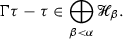
 is bounded from below without accumulation points.
 is graded by A such that each
  is a Banach space.
 such that, for every
  , one has
For  , we get

Concerning the structure group, the aim of the rest of this section is to provide a recursive construction using the symbolic notation. Let denote by  :
:

For any  we define a linear operator
  by
by

and we extend it multiplicatively to  .
.
Remark 2.2
The map \( \Gamma _{g} \) is well defined for every  as a map from
  into itself because of the fact that the rule
  is normal see [3, Def. 5.7] which implies that for every
  one has
  where J is a subset of \( \lbrace 1,\ldots ,n \rbrace \). Such operation arises in the definition of \( \Gamma _g \) on some product
  where one can replace any
  by a polynomial
  . Then we use an inductive argument to conclude that
  when
when  .
.
We define the product  recursively by:

where we have made the following abuse of notation \( (g_1(X))^{\ell } \) instead of \( \prod _{i =0}^{d} g_1(X_i)^{\ell _i} \). We will also write \( \left( X + g(X) \right) ^{\ell } \) instead of \( \prod _{i =0}^{d} \left( X_i + g(X_i) \right) ^{\ell _i} \).
Proposition 2.3
-
1.
For every
 , \( \alpha \in A \),
  and multiindex k, we have
 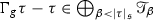 and
and  is a polynomial.
 -
2.
The set
 forms a group under the composition of linear operators from
  to
to  . Moreover, this definition coincides with that of [10, (8.17)].
 -
3.
For all
 , one has \( \Gamma _{g} \Gamma _{\bar{g}} = \Gamma _{g \circ \bar{g}} \).
  is a group and each element g has a unique inverse \( g^{-1} \) given by the recursive formula
 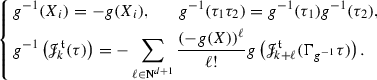 (5)
(5)The product \(\circ \) coincides with that defined in [10, Def. 8.18].
 ,
,  and multiindex k, we have
  and
and  is a polynomial.
 forms a group under the composition of linear operators from
  to
to  . Moreover, this definition coincides with that of [
 , one has
  is a group and each element g has a unique inverse
Proof
We prove the first property by induction on the construction of  . Let
. Let  . The proof is obvious for \( \tau \in \lbrace \mathbf {1},X_i,\Xi _{\mathfrak {l}} \rbrace \). Let \( \tau = \tau _{1} \tau _2 \) then we have
We apply the induction hypothesis on \( \tau _1 \) and \( \tau _2 \). Let  then the recursive definition of \( \Gamma _g \) gives:

We apply the induction hypothesis on \( \tau ' \).
Let  ,
,  . Simple computations show that
We need to check that  :
:

while

By comparing the two formulae, we obtain that \(\Gamma _{g} \Gamma _{\bar{g}}=\Gamma _{g \circ \bar{g}}\).
Let us show that \(\circ \) is associative on  , namely that \(g_1\circ (g_2\circ g_3)=(g_1\circ g_2)\circ g_3\); this is obvious if tested on X and on \(\tau \bar{\tau }\); it remains to check this formula on
  :
:

while

and again by comparing the two formulae we obtain the claim.
Let us show now that (5) defines the correct inverse in  . First of all, the neutral element in
  is clearly
  . As usual, the only non-trivial property is that
  . We have

and

where we have used a recurrence assumption in the identification \(\Gamma _{g^{-1}\circ g} \tau =\tau \). Since \(\Gamma _{\mathbf{1}^*}\) is the identity in  , we obtain that
  also forms a group.
We show now that these objects coincide with those defined in [10, section 8]. In [3, 10], the action of  on
on  is defined through the following co-action
  ,
,

We claim that

First, (6) is easily checked on \(\mathbf {1},X_i,\Xi _{\mathfrak {l}}\) and  . We check the formula on
  :
:

In [3, 10], another coproduct  is defined as follows:

In order to prove that the product \(\circ \) is the same as in [10], we need to check that for every  we have:

As usual, this formula is easily checked on \(\mathbf {1},X_i\) and on products  . We check the formula on
  :
:

\(\square \)
3 Renormalised models
We start the section by a general recursive formulation of the renormalisation group without coproduct. Then we use this formulation to construct the renormalised model. During this section, elements of the model space  are described with the symbolic notation.
3.1 A recursive formulation
Before giving the recursive definition of the renormalisation map, we precise some notations. We denote by \( \Vert \tau \Vert \) the number of times the symbols \(\Xi _{\mathfrak {l}}\) appear in \( \tau \). We extend the definitions of \( |\cdot |_{\mathfrak {s}} \) and \( \Vert \cdot \Vert \) to any linear combination \( \tau =\sum _i \alpha _i \tau _i \) of canonical basis vectors \(\tau _i\) with \( \alpha _i \ne 0 \) by
which suggests the natural conventions \(|0|_{\mathfrak {s}} = +\infty \) and \(\Vert 0\Vert = - \infty \). We also define a partial order  on
on  by setting:

Definition 3.1
A symbol \( \tau \) is an elementary symbol if it has the following form: \( \Xi _{\mathfrak {l}} \), \( X_i \) and  where \( \sigma \) is a symbol.
Proposition 3.2
Let \( \tau = \prod _i \tau _i \) such that the \( \tau _i \) are elementary symbols and such that \( \tau \) is not an elementary symbol then  .
.
Proof
We consider \( \tau = \prod _i \tau _i \) and let \( \tau _j \) an elementary symbol appearing in the previous decomposition. We define \( \bar{\tau }_{j} = \prod _{i \ne j } \tau _i \). If the product \( \bar{\tau }_{j} \) contains a term of the form  with \( \sigma \) having at least one noise or a term of the form \( \Xi _{\mathfrak {l}} \) then \( \Vert \bar{\tau }_j \Vert > 0 \) and \( \Vert \tau _j \Vert < \Vert \bar{\tau }_{j} \Vert + \Vert \tau _j \Vert = \Vert \tau \Vert \). Otherwise \( \Vert \tau _j \Vert = \Vert \tau \Vert \) but \( | \bar{\tau }_j |_{\mathfrak {s}} > 0 \) which gives \( | \tau _j |_{\mathfrak {s}} < | \tau _j|_{\mathfrak {s}} + | \bar{\tau }_j |_{\mathfrak {s}} = | \tau |_{\mathfrak {s}} \). Finally, we obtain
  . \(\square \)
Given a regularity structure  , we consider the space
  of linear maps on \( \mathcal{T}\). For our recursive formulation, we choose a subset of
  :
:
Definition 3.3
A map  is admissible if
-
1.
For every elementary symbol \( \tau \), \( R \tau = \tau \).
-
2.
For every multiindex k and any symbol \( \tau \), \( R (X^k \tau )= X^k R \tau \).
-
3.
For each
 , \( \Vert R \tau - \tau \Vert < \Vert \tau \Vert \).
 -
4.
For each
 , \( | R \tau - \tau |_{\mathfrak {s}} > | \tau |_{\mathfrak {s}} \).
 -
5.
It commutes with G: \(R \Gamma = \Gamma R\) for every \(\Gamma \in G\).
 ,
,  ,
, We denote by  the set of admissible maps. For
  , we define a renormalisation map \(M=M_R\) by:

The space of maps M constructed in this way is denoted by \( \mathfrak {R}_{ad}[\mathscr {T}] \). The main idea behind this definition is that R computes the interaction between several elements of the product \( \prod _i \tau _i \). In [10, 13], elements of the renormalisation group are described by an exponential: \( M = \exp (\sum _i C_i L_i)\) where  . When the exponential happens to be just equal to \( \mathrm {id}+ \sum _i C_i L_i \) then the link with the space \( \mathfrak {R}_{ad}[\mathscr {T}] \) is straightforward. But when several iterations of the \( L_i \) are needed even in the case of the \( L_i \) being commutative the link becomes quite unclear and hard to see. It is also unclear when M is described with a coproduct as in (24). The main difficulty occurs when one has to face nasty divergences. The recursive construction is more convenient for several purposes: it gives an explicit and a canonical way of computing the diverging constant we have to subtract. Moreover, the proof of the construction of the renormalised model is simpler than the one given in [3, 10].
Remark 3.4
The Definitions 7 as well as the convention that follows are designed in such a way that if the third and the fourth conditions of Definition 3.3 hold for canonical basis vectors \(\tau \), then they automatically hold for every  .
.
Remark 3.5
The first two conditions of Definition 3.3 guarantee that M commutes with the abstract integrator map. The third condition is crucial for the definition of M: the recursion (9) stops after a finite number of iterations since it decreases strictly the quantity \( \Vert \cdot \Vert \) and thus the partial order  . Moreover, this condition guarantees that \( R = \mathrm {id}+ L \) where L is a nilpotent map and therefore R is invertible. The fourth condition allows us to treat the analytical bounds in the definition of the model and the last condition is needed for the algebraic identities.
Remark 3.6
Note that \(M=M_R\) does not always commute with the structure group G even if R does ; we will see a counterexample with the group of the generalised KPZ equation in Sect. 5.3.
Proposition 3.7
Let  , then \( M_R \) is well-defined.
Proof
We proceed by induction using the order  . If \( \tau \in \lbrace \mathbf {1}, \Xi _{\mathfrak {l}}, X_i \rbrace \) then \( M \tau = M^{\circ } R \tau = M^{\circ } \tau = \tau \). If
  then
then

We conclude by applying the induction hypothesis on \( \tau ' \) because we have \( | \tau ' |_{\mathfrak {s}} < | \tau |_{\mathfrak {s}} \). Let  a product of elementary symbols with at least two symbols in the product, we can write
We apply the induction hypothesis on  because \( \Vert R \tau - \tau \Vert < \Vert \tau \Vert \). For \( M^{\circ } \tau \), we have
We know from Proposition 8 that for every i,  . Therefore, we apply the induction hypothesis on the \( \tau _i \). \(\square \)
Remark 3.8
In the sequel, we use the order  for all the proofs by induction on the symbols. It is possible to choose other well-order on the symbols for these proofs. One minimal condition in order to have \( M_{R} \) well defined is the following on R: for each
  , there exist \( \Xi _{\mathfrak {l}_j} \),
  and
and  such that

Then by definition of \( M_{R} \), we get:

which allows us to use an inductive argument on the \( M \sigma _i \).
Remark 3.9
There is an alternative definition of the map M. We denote by \( M_{L} \) the representation of M given by:

where the \( \tau _i \) are elementary and the map L needs to satisfy the following properties:
-
1.
For every elementary symbol \( \tau \), \( L \tau = 0 \) and for every multiindex k and symbol \( {\bar{\tau }} \), \( L X^k \bar{\tau }= X^k L {\bar{\tau }} \).
-
2.
For each
 , \( \Vert L \tau \Vert < \Vert \tau \Vert \) and \( | L \tau |_{\mathfrak {s}} > | \tau |_{\mathfrak {s}} \).
 -
3.
It commutes with G: \(L \Gamma = \Gamma L\) for every \(\Gamma \in G\).
 ,
, This properties are very similar to those of R. Noticing that the map L is nilpotent, one can check that \( R = (\mathrm {id}+L)^{-1} \) and \( M^{\circ } = M (\mathrm {id}+L) \).
3.2 Construction of the renormalised Model
We first define a metric \( d_{\mathfrak {s}} \) on  associated to the scaling \( \mathfrak {s}\) by:
We recall the definition of a smooth model in [10, Def. 2.17]:
Definition 3.10
A smooth model for a regularity structure  consists of maps:

such that \( \Gamma _{xy} \Gamma _{yz} = \Gamma _{xz} \) and \( \Pi _{x} \Gamma _{xy} = \Pi _{y} \). Moreover, for every \( \alpha \in A \) and every compact set  there exists a constant \( C_{\alpha ,\mathfrak {K}} \) such that the bounds
hold uniformly over all \( (x,y) \in \mathfrak {K} \), all \( \beta \in A \) with \( \beta \le \alpha \) and all  .
.
In the previous definition, for  , \( \Vert \tau \Vert _{\alpha } \) denotes the norm of the component of \( \tau \) in the Banach space
  . We suppose given a collection of kernels
  ,
,  satisfying the condition [10, Ass. 5.1] with \( \beta = | \mathfrak {t}|_{\mathfrak {s}} \) and a collection of noises
  such that
  . We use the notation \( D^k = \prod _{i=0}^d \frac{\partial ^{k_i}}{\partial y_i^{k_i}} \) for
  . Until the end of the section, R is an admissible map and M is a renormalisation map built from R.
As in [10], we want a renormalised model \( (\Pi ^M_{x},\Gamma _{xy}^M) \) constructed from a map \( \varvec{\Pi }\) satisfying the following property:
We define the linear map \(\varvec{\Pi }^M \) by:

where the recursive definition is the same as for M. The definition of \( \varvec{\Pi }^M \) is really close to the definition of \(\varvec{\Pi }\). The main difference is that \(\varvec{\Pi }^M \) is no longer multiplicative because we have to renormalise some ill-defined products by subtracting diverging terms which is performed by the action of R.
Remark 3.11
We have chosen the definition (12) for \(\varvec{\Pi }^{M} \) instead of (11) because it contains the definition of \(\varvec{\Pi }\) when \( R = \mathrm {id}\). Moreover, the recursive formula for the product is really close to the definition of \( \Pi _x^{M} \) and this fact is useful for the proofs.
Proposition 3.12
We have the following identities: \(\varvec{\Pi }^M \tau =\varvec{\Pi }M \tau \) and \(\varvec{\Pi }^{M^{\circ }} \tau =\varvec{\Pi }M^{\circ } \tau \).
Proof
We proceed again by induction. It’s obvious for \( \mathbf {1}\), \( X_{i} \) and \( \Xi _{\mathfrak {l}} \). For  , by the induction hypothesis the claim holds for \( \tau ' \) because
  and
and  We have:

For \( \tau = \prod _i \tau _i \) product of elementary symbols, we obtain by applying the induction hypothesis on \( R \tau - \tau \) and the \( \tau _i \):
and
which conclude the proof. \(\square \)
The renormalised model \( (\Pi ^{M},\Gamma ^{M}) \) associated to \( M=M_R \) is given by

where  is defined by

We also define

and

Proposition 3.13
The \( \Gamma ^M \) operator is also given by:
where \( F^{M}_{x} = \Gamma _{g_x^M} \). Moreover, another equivalent recursive definition is:

Proof
We have

Since by definition

then

and

so that

Therefore, \(\Gamma _{(g_{x}^{M})^{-1}}\Gamma _{g_{y}^{M}}\) satisfies the same recursive property as \(\Gamma ^M_{xy}\).
Finally, we need to prove (13). We have

where

We write \( \Gamma ^{M}_{xy} \tau = \sum _i \tau _i \) with \( |\tau _i |_{\mathfrak {s}} \le |\tau |_{\mathfrak {s}} \); note that \(\Pi ^M_{y} \tau =\Pi ^M_{x} \Gamma _{xy}^M \tau =\sum _i \Pi ^M_{x} \tau _i \), and \(A^{M}_{y,x,k,\ell }\) is zero unless  , and if this condition is satisfied then

This allows us to conclude. \(\square \)
Remark 3.14
The interest of the previous formula for \( \Gamma ^M \) is to show a strong link with the definition of \( \Pi _x^M \). Moreover it simplifies the proof of the analytical bounds of the model. Indeed, analytical bounds on \( \Pi _x^M \) give the bounds for \( \Gamma ^M \).
Proposition 3.15
The following identities hold: \( \Pi _x^M =\varvec{\Pi }^M F_x^M \) and \( \Pi _x^{M^{\circ }} =\varvec{\Pi }^{M^{\circ }} F_x^M \).
Proof
We proceed by induction. The proof is obvious for \( \tau \in \lbrace \mathbf {1},\Xi _{\mathfrak {l}},X_i \rbrace \). For  , we apply the induction hypothesis on \( \tau ' \), it follows:

It remains to check the identity on a product \( \tau = \prod _i \tau _i \) where each \(\tau _i\) is elementary. We have
since by definition \(F^{M}_{x} = \Gamma _{g_x^M} \in G \) and R commutes with G. Then by applying the induction hypothesis on \( R \tau - \tau \) and the \( \tau _i \), we have
and
\(\square \)
Proposition 3.16
If R is an admissible map then \( (\Pi ^M,\Gamma ^M) \) is a model.
Proof
The algebraic relations are given by the previous proposition. It just remains to check the analytical bounds. For \( \tau = \Xi _{\mathfrak {l}} \) or  , the proof is the same as in [10, Prop. 8.27]. For \( \tau = \prod _i \tau _i \) a product of elementary symbols, we have
We apply the induction hypothesis on the \(\tau _i \) and \( R \tau - \tau \):
It just remains the analytical bound for \( \Gamma ^M \). We proceed by induction. For \( \tau = \Xi _{\mathfrak {l}} \) or \( \tau = X_i \), the bound is obvious. Let \( \tau = \prod _i \tau _i \) where the \( \tau _i \) are elementary symbols. For \( \beta < | \tau |_{\mathfrak {s}} \), we have
For  , the recursive definition (13) gives:

Let  . If
. If  , let us write \(\Gamma _{xy}^M \tau =\tau +\sum _i \tau ^i_{xy}\) with
then if

Now, if  and
and  then
then

\(\square \)
Proposition 3.17
We suppose that for every  such that \( |\tau |_{\mathfrak {s}} < 0 \), we have \( (\Pi _x^M \tau )(x) = (\Pi _x M \tau )(x) \). Then the following identities hold: \( (\Pi _x^M \tau )(x) = (\Pi _{x} M \tau )(x) \) and \( (\Pi _x^{M^{\circ }} \tau )(x) = (\Pi _{x} M^{\circ } \tau )(x) \) for every
  .
.
Proof
We proceed by induction. For \( \tau \in \lbrace \mathbf {1},\Xi _{\mathfrak {l}},X_{i} \rbrace \), we have
For  , if \( | \tau |_{\mathfrak {s}} > 0 \) then the recursive definition of \( \Pi _x^M \) gives

For the second identity, we have used the fact that \( | M \tau ' |_{\mathfrak {s}} \ge |\tau ' |_{\mathfrak {s}} \). Otherwise, if \( |\tau |_{\mathfrak {s}} < 0 \) then the hypothesis allows us to conclude. For an elementary product \( \tau = \prod _i \tau _i \), it follows by using the induction hypothesis
\(\square \)
Remark 3.18
Proposition 3.17 is crucial for deriving the renormalised equation in many examples. Indeed, the reconstruction map  associated to the model \( (\Pi ^M,\Gamma ^M) \) is given for every
  by:
by:

because for every  , \( \Pi _x \tau \) is a function. The result of Proposition 3.17 has just been checked on examples [10, 13] and [14] but not in a general setting. In general for \(y\ne x\), \( (\Pi _x^M \tau )( y) \) is not necessarily equal to \((\Pi _x M \tau )(y)\) as mentioned in [10]. But if you carry more information on the decorated tree with an extended decoration, then this identity turns to be true see [3, Thm. 6.15].
We finish this section by establishing a link between the renormalisation maps introduced in [10] and \( \mathfrak {R}_{ad}[\mathscr {T}] \). From [10, Lem. 8.43, Thm 8.44] and [14, Thm B.1],  is the set of maps M such that
-
One has
 and \(MX^k \tau =X^k M \tau \) for all \(\mathfrak {t}\in \mathfrak {L}_+\),
  , and
, and  .
. -
Consider the (unique) linear operators
 and
and  such that \({\hat{M}}\) is an algebra morphism, \({\hat{M}} X^k=X^k\) for all k, and such that, for every
  and
and  with
with  ,
,  (14)
(14) (15)
(15)where
 is defined for every
  by
by  and
and 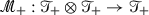 is the product on
  ,
,  . Then, for all
  , one can write \(\Delta ^{\!M}\tau = \sum \tau ^{(1)}\otimes \tau ^{(2)}\) with \(| \tau ^{(1)}|_{\mathfrak {s}} \ge | \tau |_{\mathfrak {s}}\). Having this latest property, \( \Delta ^{\!M}\) is called an upper triangular map.
 and
and  , and
, and  .
. and
and  such that
  and
and  with
with  ,
, 

 is defined for every
  by
by  and
and  is the product on
  ,
,  . Then, for all
  , one can write
 Let \( M \in \mathfrak {R}_{ad}[\mathscr {T}] \), we build two linear maps \(\Delta ^{\!M}\) and \(\Delta ^{\!M^{\circ }}\) by setting
and then recursively
as well as

We claim that if \( \Delta ^{\!M^{\circ }}\) and \(\Delta ^{\!M}\) are defined in this way, then provided that one defines \(\hat{M}\) by (14), the identity (15) holds.
Proposition 3.19
If \(M \in \mathfrak {R}_{ad}[\mathscr {T}]\), \(\Delta ^{\!M}\) is defined as above and \( \hat{M} \) is defined by (14), then the identity (15) holds and M belongs to \(\mathfrak {R}\).
Before giving the proof of Proposition 3.19, we need to rewrite (15). Indeed, the identity (15) is equivalent to

where  is the antipode associated to \( \Delta ^{\!+}\) defined by:

The identity (18) is the consequence of the following lemma:
Lemma 3.20
Let  given by

then D is invertible and \( D^{-1} \) is given by

Proof
We have by using the fact that \( (\Delta \otimes \mathrm {id}) \Delta = (\mathrm {id}\otimes \Delta ^{\!+}) \Delta \) and 

Now it follows with the identities  and \( (\mathrm {id}\otimes \mathbf {1}^{*})\Delta \tau = (\tau \otimes \mathbf {1}) \)

Using the same properties, we prove that \( D D^{-1} = \mathrm {id}\otimes \mathrm {id}\). \(\square \)
Remark 3.21
The previous lemma gives an explicit expression of the inverse of D. It is a refinement of [10, Proposition 8.38] which proves the fact that D is invertible.
Remark 3.22
The equivalence between (18) and (15) is in the strong sense that (18) holds for any given symbol \(\tau \) if and only if (15) holds for the same symbol \(\tau \).
Before giving the proof of Proposition 3.19, we provide some identities concerning the antipode  . Regarding the antipode
  , one has the recursive definition

which gives

As a consequence of this, one has the identity

To see this, simply apply on both sides in (19) the antipode  .
.
Proof Proposition 3.19
Since (14) holds by definition and it is straightforward to verify that \(\Delta ^{\!M}\) is upper triangular (just proceed by induction using (17) and (16)), we only need to verify that (15), or equivalently (18), holds. For this, we first note that since \(\Delta ^{\!M}= \Delta ^{\!M^{\circ }}R\), \(M = M^\circ R\), R commutes with \(\Delta \), and since R is invertible by assumption, (18) is equivalent to the identity

and it is this identity that we proceed to prove now. Both sides in (21) are morphisms so that, by induction, it is sufficient to show that if (21) holds for some element \(\tau \), then it also holds for  . (The fact that it holds for \(\mathbf {1}\), \(X_i\) and \(\Xi _{\mathfrak {l}}\) is easy to verify.)
Starting from (17), we first use (14) and the fact that \(\Delta ^{\!M}\) and \(\Delta ^{\!M^{\circ }}\) agree on elements of the form  to rewrite
  as
as

where the sum runs over all multiindices \(\ell \) (but only finitely many terms in the sum are non-zero). By (20), we have

Recall that by Remark 3.22, the induction hypothesis implies that (15) holds, so that we finally conclude that

Using again the induction hypothesis, but this time in its form (18), we thus obtain from (22) the identity

At this stage, we see that we can use the definition of \(\Delta \) to combine the first and the last term, yielding

We now rewrite the last term

Inserting this into the above expression and using the definition of \(\Delta \) finally yields (21) as required, thus concluding the proof.
4 Link with the renormalisation group
In this section, we establish a link between the renormalisation group \( \mathfrak {R}[\mathscr {T}] \) defined in [3] and the maps M constructed from admissible maps R.
Theorem 4.1
One has \( \mathfrak {R}[\mathscr {T}] \subset \mathfrak {R}_{ad}[\mathscr {T}]\).
The outline of this section is the following. We first start by recalling the definition of \( \mathfrak {R}[\mathscr {T}] \) and then we show that these maps are of the form \( M^{\circ } R \). Then we prove the commutative property with the structure group and we give a proof of Theorem 4.1. Finally, we derive a recursive formula.
4.1 The renormalisation group
Before giving the definition of \( \mathfrak {R}[\mathscr {T}] \), we need to introduce some notations. Let  the free commutative algebra generated by \( B_{\circ }\). We denote by \( \cdot \) the forest product associated to this algebra. Elements of
  are of the form \( (F,\mathfrak {n},\mathfrak {e}) \) where F is now a forest. Then for the forest product we have:
where the sums \( {\bar{\mathfrak {n}}} + \mathfrak {n}\) and \( {\bar{\mathfrak {e}}} + \mathfrak {e}\) mean that decorations defined on one of the forests are extended to the disjoint union by setting them to vanish on the other forest. Then we set  where
where  is the ideal of
  generated by \( \lbrace \tau \in B_{\circ } \; : \; | \tau |_{\mathfrak {s}}\ge 0 \rbrace \). Then the map
  defined in [3] is given for
  by:
by:

where
-
For \( C \subset D \) and
 , let
, let  the restriction of f to C.
 -
The first sum runs over \( \mathfrak {A}(T) \), all subgraphs A of T, A may be empty. The second sum runs over all
 and
and  where \( \partial (A,F) \) denotes the edges in \( E_T {\setminus } E_A \) that are adjacent to \( N_A \).
 -
We write
 for the tree obtained by contracting the connected components of A. Then we have an action on the decorations in the sense that for
  such that \( A \subset T \) one has: \( [f]_A(x) = \sum _{x \sim _{A} y} f(y) \) where x is an equivalence class of \( \sim _A \) and \( x \sim _A y \) means that x and y are connected in A. For
  , we define for every \( x \in N_T \), \( (\pi g)(x) = \sum _{e=(x,y) \in E_T} g(x)\).
 , let
, let  the restriction of f to C.
 and
and  where
where  for the tree obtained by contracting the connected components of A. Then we have an action on the decorations in the sense that for
  such that
  , we define for every
 Then one can turn this map into a coproduct  and obtain a Hopf algebra for
  endowed with this coproduct and the forest product see [3, Prop. 5.35]. The main difference here is that we do not consider extended decorations but the results for the Hopf algebra are the same as in [3]. This allows us to consider the group of character of this Hopf algebra denoted by
  which is the set of multiplicative elements of
  the dual of
  endowed with the convolution product \( \circ \) described below:

where  is the antipode for \( \Delta ^{\!-}\). In comparison to [3], we add the assumptions on
  that every
  is zero on \( \hat{B}_{\circ } \cap B_{\circ }^{-} \) and on every \(T^{\mathfrak {n}}_{\mathfrak {e}} \in B_{\circ }^{-} \) such that \( \mathfrak {n}(\varrho _T) \ne 0 \) where \( \hat{B}_{\circ } \) are the planted trees of \( B_{\circ } \) and \( B^{-}_{\circ } \) are the elements of \( B_{\circ } \) with negative degree. Actually it is easy to check that these assumptions define a subgroup of
  . Then the renormalisation group \( \mathfrak {R}[\mathscr {T}] \) is given by:

In order to rewrite these maps \( M_{\ell } \) in terms of some \( M^{\circ } \) and R, we need to derive a factorisation of the map \( \Delta ^{\!-}\). We denote the forest product by \( \cdot \) and the empty forest by \( \mathbf {1}_1 \).
Definition 4.2
For all trees T we denote by \(\mathfrak {A}^\circ (T)\) the family of all (possibly empty) \(A\in \mathfrak {A}(T)\) such that if \(A=\{S_1,\ldots ,S_k\}\) then \(\varrho _{S_i}\ne \varrho _T\) for all \(i=1,\ldots ,k\). For all forests F with \(F=T_1\cdot T_2\cdots T_n\) we set
and \(\mathfrak {A}^\circ (\mathbf {1}):=\emptyset \). We also define \( \mathfrak {A}^r(T) \) containing the empty forest and the non-empty forests A such that \( A = \lbrace S \rbrace \) and \( \varrho _S = \varrho _T \).
We define the maps \( \Delta ^{\!-}_{\circ } \) (resp. \( \Delta ^{\!-}_r \)) as the same as \( \Delta ^{\!-}\) by replacing \( \mathfrak {A}(T) \) in (23) by \( \mathfrak {A}^{\circ }(T) \)(resp. \( \mathfrak {A}^r(T) \)).
Proposition 4.3
The map \(\Delta ^{\!-}_{\circ }\) is multiplicative on  , i.e. \(\Delta ^{\!-}_{\circ }(\tau _1\tau _2)=(\Delta ^{\!-}_{\circ }\tau _1)(\Delta ^{\!-}_{\circ }\tau _2)\) for all
  , where we consider on
  the product
Proof
We introduce \({\hat{\Pi }}:\hat{B}_{\circ }\mapsto B_{\circ }\) the map which associates to a planted decorated tree \(T^\mathfrak {n}_\mathfrak {e}\) a decorated tree obtained by erasing the only edge \(e=(\varrho ,y)\) incident to the root \(\varrho \) in T and setting the root to be y.
Since all decorated trees are products of elementary trees, it is enough to prove that for \(\tau _1,\ldots ,\tau _m\in \hat{B}_{\circ }\) such that \( \tau _1 \ldots \tau _m \in B_{\circ } \) we have \(\Delta _{\circ }(\tau _1\cdots \tau _m)=(\Delta _{\circ }\tau _1)\cdots (\Delta _{\circ }\tau _m)\). It is easy to see that for all \(T^\mathfrak {n}_\mathfrak {e}\in \hat{B}_{\circ }\)

where as above \(\varrho \) is the root of \(T^\mathfrak {n}_\mathfrak {e}\) and \(e=(\varrho ,y)\) is the only edge incident to \(\varrho \).
Now if \(T^\mathfrak {n}_\mathfrak {e}=\tau _1\cdots \tau _m\in B_{\circ }\) with \(\tau _1,\ldots ,\tau _m\in \hat{B}_{\circ }\), then we have a canonical bijection between \(\mathfrak {A}^{\circ }(T^\mathfrak {n}_\mathfrak {e})\) and \(\mathfrak {A}({\hat{\Pi }} \tau _1)\times \cdots \times \mathfrak {A}({\hat{\Pi }}\tau _m)\) and the numerical coefficients factorise nicely, so that

\(\square \)
Proposition 4.4
Let  , \(\phi \otimes \bar{\phi }\mapsto \phi \cdot \bar{\phi }\). Then

holds on  .
.
Proof
By multiplicativity on  , it is enough to prove the equality on all \(T_\mathfrak {e}^\mathfrak {n}\in B_{\circ }\). Note that

and therefore

At this point, we note that since  , \(\mathfrak {e}_A\) and \(\mathfrak {e}_B\) have disjoint support so that \(\mathfrak {e}_A!\mathfrak {e}_B! = (\mathfrak {e}_A + \mathfrak {e}_B)!\). Similarly, thanks to the fact that \(\mathfrak {n}_B\) has support away from the root of
  , one has
so that
We note also that the map \((A,B)\mapsto C = A \cup B\) is a bijection between  and \(\mathfrak {A}(T)\), since every \(C \in \mathfrak {A}(T)\) is either in \(\mathfrak {A}^\circ (T)\) (if none of the subtrees touches the root of T), or of the form \(\{S\} \cup B\), where \(\varrho _S=\varrho _T\) and
  . Moreover setting, \(\mathfrak {e}_C = \mathfrak {e}_A + \mathfrak {e}_B\) and \(\mathfrak {n}_C = \mathfrak {n}_A + \mathfrak {n}_B\), the above sum can also be rewritten as

This concludes the proof. \(\square \)
Corollary 4.5
Let  , \(R_\ell {\mathop {=}\limits ^{\mathrm{def}}}(\ell \otimes \mathrm {id})\Delta ^{\!-}_r\) and \(M^{\circ }_\ell {\mathop {=}\limits ^{\mathrm{def}}}(\ell \otimes \mathrm {id})\Delta ^{\!-}_{\circ }\). Then \( M_{\ell } = M^\circ _{\ell } R_{\ell } \).
Proof
Note that
Now, since  is multiplicative, we obtain

\(\square \)
Through the next tree T, we illustrate the Proposition 4.4 by considering \( A = \lbrace S_1, S_2, S_3 \rbrace \in \mathfrak {A}(T) \):

We have \( \lbrace S_3 \rbrace \in \mathfrak {A}^r(T) \) and  .
.
In order to be able to prove the next proposition, we recall the definition of \( \Delta _2 \) given in [3]. The map  is given for
  by:
by:

where \( \mathfrak {A}^+(T) \) is the set of subtrees A of T such that \( \varrho _{A} = \varrho _T \). Then one obtains \( \Delta ^{\!+}\) by applying \( \Pi _+ \): \( \Delta ^{\!+}= (\mathrm {id}\otimes \Pi _+ ) \Delta _2 \).
Proposition 4.6
We have
Moreover for all  , \( R_{\ell } \) commutes with G.
Proof
The result follows from the identity:
Indeed, one has \( \Delta ^{\!+}= \left( \mathrm {id}\otimes \Pi _+ \right) \Delta _2 \) which gives:
So it remains to prove (27). We first notice the next identity between \( \Delta ^{\!-}_r \) and \( \Delta _2 \):

where  is the map which sends \( (T,2)^{\mathfrak {n}}_{\mathfrak {e}} \) to \( T^{\mathfrak {n}}_{\mathfrak {e}} \) or which removes the colour two at the root and
  is the projection which maps single node without decoration to the empty forest, any other tree is identified with the forest containing only this tree. The map \( \tilde{\Pi } \) is extended multiplicatively to the space
  . Then (27) follows from the co-associativity of \(\Delta _2\) proved in [3]. Indeed by setting \( \tilde{\Pi }_- = \Pi _- \circ \tilde{\Pi }\), we have

Now for all  and
and 
\(\square \)
We finish this subsection by the proof of the Theorem 4.1:
Proof Theorem 4.1
Let \( M \in \mathfrak {R}[\mathscr {T}] \), there exists  such that
From Corollary 4.5, we know that \( M_{\ell } = M^{\circ }_{\ell } R_{\ell } \) where
We need to check that  and that \( M^{\circ }_{\ell } \) satisfies the recursive definition (9). For \( M^{\circ }_{\ell } \), this property comes from Proposition 4.3 and from (25) which gives for every
  :
:

For \( R_{\ell } \), we first notice that for every  , \(\Delta ^{\!-}_{r} \tau \) is of the form \( \mathbf {1}_{1} \otimes \tau + \sum _i \tau _i^{(1)} \otimes \tau ^{(2)}_i \) where \( | \tau |_{\mathfrak {s}} = | \tau _i^{(1)} |_{\mathfrak {s}} + | \tau _i^{(2)} |_{\mathfrak {s}} \) and \( || \tau || = || \tau _i^{(1)} || + || \tau _i^{(2)} || \), \( || \tau _i^{(2)} || < || \tau ||\). The tree \( \tau _i^{(1)} \) is of negative degree thus \( | \tau |_{\mathfrak {s}} \ge | \tau _i^{(2)} |_{\mathfrak {s}} \) and we get the following properties:\( \Vert R_{\ell } \tau - \tau \Vert < \Vert \tau \Vert \) and \(\vert R_{\ell } \tau - \tau \vert _{\mathfrak {s}} < \vert \tau \vert _{\mathfrak {s}} \). Let
  , then by definition of
  we get
  which yields:

As the same any power of X at the root is killed by the character \( \ell \) which proves the identity \( R_{\ell } X^k \tau = X^k R_{\ell } \tau \) for every  . The fact that \( R_{\ell } \) commutes with the structure group proceeds from Proposition 4.6. From all these properties, we have \( M_{\ell } \in \mathfrak {R}_{ad}[\mathscr {T}] \) which concludes the proof. \(\square \)
4.2 Recursive formula for the renormalisation group
We want to derive a recursive formula for \( \Delta ^{\!-}\) by using the symbolic notation. The recursive formulation is based on the tree product and the inductive definition of the trees. The main difficulty at this point is that one can derive easily a recursive formula for \( \Delta ^{\!+}\) which is multiplicative for the tree product but not for \( \Delta ^{\!-}\). In order to recover this multiplicativity, we define a slight modification \( {\hat{\Delta }}_1 \) of \( \Delta ^{\!-}\) by adding more information. The main idea is to distinguish a tree in a forest. This formulation allows to have a recursive definition for the two coproducts \( \Delta ^{\!-}\) and \( \Delta ^{\!+}\).
Definition 4.7
We define \( \mathfrak {F}_{\varrho }\) the space of \( (F,\mathfrak {n},\mathfrak {e},\varrho ) = (F_{\mathfrak {e}}^{\mathfrak {n}},\varrho ) \) such that F is non- empty and such that \( \varrho \) is the root of one connected component \( T_{\varrho } \) of F. The space \( \mathfrak {F}_{\varrho } \) can be viewed as the non-empty decorated forests where we distinguish one tree. We endow this space with a product \( \star \) defined as follows:
where \( F_{\varrho }^{c} = F {\setminus } \lbrace T_{\varrho } \rbrace \). We have also identified the two roots \( \varrho \) and \( {\bar{\varrho }} \) with \( \tilde{\varrho } \) which means that \( \mathfrak {n}(\tilde{\varrho }) = \mathfrak {n}(\varrho ) + {\bar{\mathfrak {n}}}({\bar{\varrho }}) \). We denote by \( \mathfrak {T}_{\varrho } \) the forests \( (F^{\mathfrak {n}}_{\mathfrak {e}},\varrho ) \in \mathfrak {F}_{\varrho } \) such that \( F_{\varrho }^{c} \) is empty. Then we define a canonical injection \( \iota _{\varrho } : \mathfrak {T}\rightarrow \mathfrak {T}_{\varrho } \), \( \iota _{\varrho }(T_{\mathfrak {e}}^{\mathfrak {n}}) = ( T_{\mathfrak {e}}^{\mathfrak {n}}, \varrho _T ) \) and we denote by \( \Pi ^{\varrho } \) its left inverse which is defined by:
Definition 4.8
We define \( \mathfrak {A}(F,\varrho ) \) as the family of all \( (A,\varrho ) \in \mathfrak {F}_{\varrho } \) such that \( A \in \mathfrak {A}(F)\) and A contains all the nodes of the forest F.
Remark 4.9
In the Definition 4.8, we extract all the nodes because we want to derive a recursive formula for \( \Delta ^{\!-}\) which means that one is not able to decide immediately during the recursive procedure in (31) if one node will belong to a tree extracted by \( \Delta ^{\!-}\).
We define \( {\hat{\Delta }}_1 : \mathfrak {F}_{\varrho } \rightarrow \mathfrak {F}_{\varrho } \otimes \mathfrak {F}_{\varrho } \) in the following way:

The infinite sum makes sense as the same as in [3] by using the bigraded structure of \( \mathfrak {F}_{\varrho }\) and the fact that \( \hat{\Delta }_1 \) is a triangular map.
Proposition 4.10
The map \( {\hat{\Delta }}_1 \) is multiplicative for \( \star \) and one has on \( \mathfrak {F}_{\varrho } \):
Proof
The multiplicativity comes from the fact that
The rest of the proof can be seen as a consequence of the co-associativity results obtained in [3] see Remark 4.11. In order to avoid the introduction of too much notations, we provide a direct proof in the appendix using the formula (31) with the symbolic notation. \(\square \)
Remark 4.11
One can define \( \mathfrak {A}(F,\varrho ) \) using the formalism of the colours developed in [3] by \( \mathfrak {A}_1(F,\hat{F},\varrho ) \) where in this case \( \hat{F}^{-1}(1) = N_{F} \) and with the difference that we need to carry more information by keeping track of the root of one tree in F. This means that elements of \( \mathfrak {F}_{\varrho } \) have all their nodes coloured by the colour 1. Then for the definition of the coproduct, all the nodes are extracted. We can then apply [3, Prop. 3.9] without the extended decoration in order to recover the Proposition 4.10.
Remark 4.12
This coproduct \( {\hat{\Delta }}_1 \) contains at the same time the Connes-Kreimer coproduct and the extraction-contraction coproduct. In the sense that if we forget the root \( \varrho \), we obtain a variant of the extraction-contraction coproduct where each node needs to be in one extracted subtree. On the other hand, if we quotient by the elements \( (F,\varrho ) \) such that F contains a tree with a root different from \( \varrho \), we have the Connes-Kreimer coproduct. We make this statement more precise in Proposition 4.15.
From Corollary 29, we can derive a general recursive formula by using the symbolic notation. Before giving it, we need to encode \( (F^{\mathfrak {n}}_{\mathfrak {e}},\varrho ) \). For that, we introduce the new symbol \( \mathscr {C}\) which is a map from \( \mathfrak {F}_{\varrho } \) into itself. Now \( (\lbrace T_{\varrho }, \; T_1, \; \ldots , \;T_n \rbrace , \varrho ) \) is given by \( T_{\varrho } \prod _{i=1}^n \mathscr {C}(T_i) \) where \( T_{\varrho } \) is the tree with root \( \varrho \). Let \( (F^{\mathfrak {n}}_{\mathfrak {e}},\tilde{\varrho }), ({\bar{F}}^{{\bar{\mathfrak {n}}}}_{\bar{\mathfrak {e}}},{\bar{\varrho }}) \in \mathfrak {F}_{\varrho } \), the product \( \star \) is given by:
Then the properties of the symbol \( \mathscr {C}\) are:
-
1.
The product \( \mathscr {C}(T)\mathscr {C}({\bar{T}}) \) is associative and commutative as the product on the forests. Moreover, the map \( \mathscr {C}\) is multiplicative for the product of forests, \( \mathscr {C}(F \sqcup {\bar{F}}) = \mathscr {C}(F ) \mathscr {C}({\bar{F}}) \).
-
2.
The symbol \( \mathscr {C}\) is also defined as an operator on \( (F^{\mathfrak {n}}_{\mathfrak {e}},\varrho ) \) in the sense that \( \mathscr {C}((F^{\mathfrak {n}}_{\mathfrak {e}},\varrho )) \) is the forest \( (F^{\mathfrak {n}}_{\mathfrak {e}} \sqcup \lbrace \bullet \rbrace ,\bullet ) \). Using only the symbolic notation, this can be expressed as:
$$\begin{aligned} \mathscr {C}(T_{\varrho } \mathscr {C}( F_{\varrho }^{c})) = \mathscr {C}( T_{\varrho }) \mathscr {C}( F_{\varrho }^{c}). \end{aligned}$$ -
3.
The operator
 is extended by acting only on the tree with the root \( \varrho \) in \( (F^{\mathfrak {n}}_{\mathfrak {e}},\varrho ) \):
 is extended by acting only on the tree with the root
With these properties, we define the map \( {\hat{\Delta }}_1 \):

where \( \mathbf {1}\) corresponds here to \( (\lbrace \bullet \rbrace ,\bullet ) \). We make an abuse of notations by identifying \( (T,\varrho _T) \) and T when T is a tree.
The previous recursive construction and the properties of the map \( \mathscr {C}\) can be explained graphically. We concentrate ourself on the shape and we omit the decorations. If we look at one term \( \tau _1 \otimes \tau _2 \) appearing in the decomposition of \( {\hat{\Delta }}_1 \tau \) for some tree \( \tau \) then \( \tau _1 \) is of the form \( \bar{\tau }\prod _j \mathscr {C}({\bar{\tau }}_j)\). We colour trees of the form \( \mathscr {C}({\bar{\tau }}_j) \) in red and leave \( {\bar{\tau }} \) in black in the next example:

In the next proposition, we prove the equivalence between the recursive definition on the symbols and the definition (29) .
Proposition 4.13
The definitions (29) and (31) coincide.
Proof
The fact that \({\hat{\Delta }}_1 \mathbf {1}= \mathbf {1}\otimes \mathbf {1}\) follows immediately from the definitions. The element \(X^k \) is encoded by the tree consisting of just a root, but with label k: \( ( \lbrace \bullet ^k \rbrace ,\bullet ) \). One then has \(A = \lbrace \bullet \rbrace \) and \(\mathfrak {e}_A = 0\), while \(\mathfrak {n}_A\) runs over all possible decorations for the root. This shows that (29) yields in this case
which is as required. It now remains to verify that the recursive identities hold as well. The coproduct \( {\hat{\Delta }}_1 \) is multiplicative for \( \star \). Thus we can restrict ourselves to \({\hat{\Delta }}_1 \mathscr {C}(T^{\mathfrak {n}}_\mathfrak {e}) \) and  where \( T^{\mathfrak {n}}_{\mathfrak {e}} \) is a decorated tree. For the first, we just notice that:
where \( \varrho \) is different from the root \( \varrho _T \) of T and \( (\mathrm {id},\varrho ) \) replaces the root by \( \varrho \) and adds \( \varrho \) to the forest. The operator \( (\mathrm {id}, \varrho ) \) is identified with  . It remains to consider
  . It follows from the definitions that by denoting \( \varrho \) the root of

This decomposition translates the belonging or not of the edge  to
to  . Given \( (A,\varrho _{T}) \in \mathfrak {A}(T,\varrho _T)\), since the root-decoration of
  is 0, the set of all possible node-labels \(\mathfrak {n}_A\) for
  appearing in (29) for
  coincides with those appearing in the expression for \({\hat{\Delta }}_1 T^{\mathfrak {n}}_\mathfrak {e}\). Furthermore, it follows from the definitions that for any such A one has

so that we have the identity

because \( \mathfrak {n}(\varrho ) =0 \) so that \(\mathfrak {n}_{\varrho }\) is a zero ( \(\mathfrak {n}(\varrho ) - \mathfrak {n}_{\varrho } \ge 0 \) ) . Note now that \(\mathfrak {e}_{\varrho }\) consists of a single decoration (say \(\ell \)), supported on \(e_\varrho \). As a consequence, we can rewrite the above as

\(\square \)
Remark 4.14
We can derive a recursive formula for \( {\hat{\Delta }}_1 \) with the extended decorations introduced in [3]:

where \( \mathbf {1}_{\mathfrak {o}} \) is the tree with one node having the extended decoration  .
.
Before making the link between \( {\hat{\Delta }}_1 \) and the maps \( \Delta ^{\!-}\), \( \Delta ^{\!+}\), we introduce some notations. We denote by  the map acting on trees by sending \( T^{\mathfrak {n}}_{\mathfrak {e}} \) to \( (T,2)^{\mathfrak {n}}_{\mathfrak {e}} \) or equivalently by colouring the root with the colour 2. Then we define the map \( \Pi _{\mathfrak {T}} : \mathfrak {F}_{\varrho } \rightarrow \mathfrak {T}_{\varrho } \) by sending \( (F,\varrho ) \) to \( (T_{\varrho },\varrho ) \) when \( F = T_{\varrho } \cdot \bullet \cdot \cdots \cdot \bullet \) and zero otherwise. In the next proposition, we also use the map
  defined for the identity (28). This map allows to remove the isolated nodes.
Proposition 4.15
One has on  :
:

Proof
The proof follows from the expressions of \( \Delta ^{\!-}\), \( \Delta ^{\!+}\) and \( {\hat{\Delta }}_1 \) respectively given in (23), (26) and (29). Indeed, we have a bijection between elements of \( \mathfrak {A}(F,\varrho ) \) which are of the form \( (T_{\varrho } \cdot \bullet \cdot \cdots \cdot \bullet , \varrho ) \) and \( \mathfrak {A}^+(T) \). We also have a bijection between the \( A\in \mathfrak {A}(T) \) which don’t have any isolated nodes and \( \mathfrak {A}(F,\varrho ) \). These bijections come from the fact that all the nodes are extracted in the definition of \( \mathfrak {A}(F,\varrho ) \). \(\square \)
5 Examples of renormalised models
For the examples of this section, we define the renormalisation map \( M_{R} \) by using an admissible map \( R_{\ell } = (\ell \otimes \mathrm {id}) \Delta ^{\!-}_r \) with  . Moreover for each example, we describe the structure and we look at the following properties which a model could verify or not:
-
(a)
The map M commutes with G .
-
(b)
For every symbol \( \tau \), \( \Pi _x^M \tau = \Pi _x M \tau \).
-
(c)
For every symbol \( \tau \), \( (\Pi _x^M \tau ) (x) = (\Pi _x M \tau ) (x) \).
Remark 5.1
In this section, we will give examples which do not verify the first two properties. But the last one is verified by all the examples. In the framework of the extended structure, we directly have the second property see [3, Thm 6.15].
We start with a toy model on the Wick renormalisation then we move on to examples in singular SPDEs.
5.1 Hermite polynomials
We look at a very simple example: the powers of a standard Gaussian random variable \( \xi \) with zero mean and covariance \( c^2\), which can be interpreted as a white noise on a singleton \(\{x\}\). The space  is given as the linear span of
  and \(G = \lbrace \mathrm {id}\rbrace \) . Given the natural definition
we want to find M such that the renormalised n-th power of \( \xi \) is the Wick product:
where \(H_n\) are generalised Hermite polynomials: \(H_0=1\), \( H_{n+1}(x,c) = x H_{n}(x,c) -c^2 H'_{n}(x,c) \). One natural way of defining M is \( M = \exp (-R_{\ell }) \) where \( R_{\ell } = (\ell \otimes \mathrm {id}) \Delta ^{\!-}_r \) and  . The map \( \Delta ^{\!-}_r \) is defined on \( \Xi ^n \) by:
This map can be expressed in our general setting with the same subset \( \mathfrak {A}^r(T) \). But in that case, we do not have any decorations. In the next example, we will encode \( \Xi ^n \) with a set of n leaves. A rooted subtree is identified with a subset of leaves. We present one term in the decomposition of \( \Delta ^{\!-}_r \Xi ^8 \) which is in the support of \( \ell \):

We have removed the set \( \lbrace \ell _{3}, \ell _{7} \rbrace \) from the term \( \Xi ^8 \). Then \( \varvec{\Pi }^M \) is given by:
By definition, this example verifies all the three properties (a), (b) and (c). We are able to provide a description of M:
Proposition 5.2
The map M is given by:
where
Proof
We use the following lemma: \(\square \)
Lemma 5.3
For every  \( \frac{R^k}{k!} = ( f_k \otimes \mathrm {id}) \Delta ^{\!-}_r \), where
Proof
We proceed by recurrence. It is obvious for \( k =1 \). Let  , we suppose the property true for this integer. We have for every
From the previous lemma, we deduce that \( \ell _{wick} = \mathbf {1}^{*} + \sum _{k \ge 1} (-1)^k f_k \) which concludes the proof. \(\square \)
Remark 5.4
In this particular case, we look at a recursive formulation of \( M = M^{\circ } R \), R turns out to be equal to M because \( M^{\circ } \) is the identity on  . This is also the reason why \( \ell _{wick} \) has a complicate expression in comparison to \( \ell \).
5.2 The KPZ equation
The KPZ equation is given on  by
by
where \( \xi \) is the space-time white noise. In this equation, there is only one noise denoted by \( \Xi \) in the symbolic notation. Moreover, we denote by  the abstract integrator associated to the heat kernel K. The scaling \( \mathfrak {s}\) is the parabolic scaling (2, 1) . In the sequel, we make the following abuse of notation
  . The renormalisation group for the KPZ equation has been introduced in [9] and it has been given in the setting of regularity structure in [10]. We first present the normal and complete rule
  used for building
  following [3, Sec. 5.4]:

The admissible map \( R = R_{kpz} \) associated to the map M is given by \( R_{kpz} = ( \ell _{kpz} \otimes \mathrm {id}) \Delta ^{\!-}_r \) where \( \ell _{kpz} \) is non zero for:

For the next Proposition 5.5, we need to work with a different rule:

We consider a new space  generated by this rule such that the symbol
  is zero whenever \( \tau \) is a polynomial. This space was used in [10]. In practice for the expansion of the solution, we work with a truncated version of it by considering only the symbols below a certain degree. It is the same for
  . Then only a finite number of polynomials appears when we apply the structure group on
  . We make the same assumption as in [10] that the kernel K associated to
  annihilates polynomials up to a certain order bigger than the order of the truncation.
Proposition 5.5
The map \( M = M_{R_{kpz}} \) satisfies the properties (a), (b) and (c).
Proof
For proving the first two properties (a) and (b), we need the following lemma: \(\square \)
Lemma 5.6
For every symbol \( \tau \), \( M^{\circ } \tau = \tau \) and there exists a polynomial \( P_{\tau } \) such that: \( M \tau = \tau + P_{\tau }(X)\).
Proof
We proceed by induction. It is obvious for \( X_i \) and \( \Xi \). For  , we apply the induction hypothesis on \( \tau ' \) which gives

Let \( \tau = \prod _i \tau _i \) a product of elementary symbols. From the induction hypothesis on the \( \tau _i \), it follows
Then \( R \tau - \tau \) is non zero if one element in the support of \( \ell _{kpz} \) is a subtree of \( \tau \). Necessarily, \( \tau \) should be of the form
-
 ,
, -
 ,
, -
 ,
,
 ,
, ,
, ,
,where the \( \tau _i \) belong to  . By looking, at the rule available in
  , we deduce that the \( \tau _i \) should be monomials of the form \( X^k \). Therefore, \( R \tau - \tau \) is a polynomial which allows us to conclude.
For the property (a), we proceed by induction and we also prove that \( {M^{\circ }} \) commutes with G . Let \( \Gamma \in G \), the proof is obvious for \( X_i \) and \( \Xi \). Let  , it happens

On the other hand, we have

Using the previous lemma, it follows  and
and  which give the result. The same proof works for \( M^{\circ } \).
Let \( \tau = \prod _i \tau _i \) a product of elementary symbols, we have
where we have used the fact that M commutes with \( \Gamma \) on the \( \tau _i \) and \( R \tau \) which comes from the induction hypothesis and the fact that R commutes with G . For the property (b), we proceed as the same by induction. The only difficult point is for  . We have by applying the induction hypothesis, the previous lemma on \( \tau ' \) and using the fact that K integrates to zero against polynomials

which allow us to conclude. \(\square \)
5.3 The generalised KPZ
The equation contains the previous equation and it is given by:
The rule  for building
  is given by:

where  is a shorthand notation for
  where
where  is repeated \( \ell \) times. The admissible map \( R_{gkpz} \) associated to the generalised KPZ is defined by \( R_{gkpz} = ( \ell _{gkpz} \otimes \mathrm {id}) \Delta ^{\!-}_r \) where \( \ell _{gkpz} \) is non zero on trees with negative degree which do not contain any X.
Proposition 5.7
The map \( M = M_{gkpz} \) satisfies only the property (c).
Proof
One counterexample, for the properties (a) and (b) is given by:  , we have

where  . Now
. Now  is a polynomial different from zero. Similarly, one can check that \( \Pi _x^M \tau \ne \Pi _x M \tau \). For the property (c), we use the Proposition 3.17. We need to check that property on every
  with negative degree. Such terms do not exist. Then

and  for
for  . \(\square \)
5.4 The stochastic quantization
The stochastic quantization is given in dimension 3 by:
and has been studied in [10]. The rule  for building
  is:
is:

The admissible map \( R_{qua} \) associated to the stochastic quantization is defined by \( R_{qua} = ( \ell _{qua} \otimes \mathrm {id}) \Delta ^{\!-}_r \) where \( \ell _{qua} \) is non zero for:

Proposition 5.8
The map \( M=M_{qua} \) satisfies only the property (c).
Proof
For the properties (a) and (b), a good counterexample is  . For the property (c),
  Then it is obvious that
  . \(\square \)
References
Bruned, Y., Chandra, A., Chevyrev, I., Hairer, M.: Renormalising SPDEs in regularity structures. ArXiv e-prints (2017). arXiv:1711.10239
Bruned, Y., Chevyrev, I., Friz, P.K., Preiss, R.: A rough path perspective on renormalization. ArXiv e-prints (2017). arXiv:1701.01152
Bruned, Y., Hairer, M., Zambotti, L.: Algebraic renormalisation of regularity structures. ArXiv e-prints (2016). arXiv:1610.08468
Calaque, D., Ebrahimi-Fard, K., Manchon, D.: Two interacting Hopf algebras of trees: a Hopf-algebraic approach to composition and substitution of B-series. Adv. Appl. Math 47(2), 282–308 (2011). https://doi.org/10.1016/j.aam.2009.08.003. arXiv:0806.2238
Chandra, A., Hairer, M.: An analytic BPHZ theorem for regularity structures. ArXiv e-prints (2016). arXiv:1612.08138
Chartier, P., Hairer, E., Vilmart, G.: A substitution law for B-series vector fields. Research Report RR-5498, INRIA (2005). https://hal.inria.fr/inria-00070509
Chartier, P., Hairer, E., Vilmart, G.: Algebraic structures of B-series. Found. Comput. Math. 10(4), 407–427 (2010). https://doi.org/10.1007/s10208-010-9065-1
Gubinelli, M.: Controlling rough paths. J. Funct. Anal. 216(1), 86–140 (2004). https://doi.org/10.1016/j.jfa.2004.01.002
Hairer, M.: Solving the KPZ equation. Ann. Math. (2) 178(2), 559–664 (2013). https://doi.org/10.4007/annals.2013.178.2.4. arXiv:1109.6811
Hairer, M.: A theory of regularity structures. Invent. Math 198(2), 269–504 (2014). https://doi.org/10.1007/s00222-014-0505-4. arXiv:1303.5113
Hairer, M.: The motion of a random string. ArXiv e-prints (2016). arXiv:1605.02192
Hoshino, M.: KPZ equation with fractional derivatives of white noise. Stoch. Partial Differ. Equ. Anal. Comput. 4(4), 827–890 (2016). https://doi.org/10.1007/s40072-016-0078-x. arXiv:1602.04570
Hairer, M., Pardoux, É.: A Wong–Zakai theorem for stochastic PDEs. J. Math. Soc. Jpn. 67(4), 1551–1604 (2015). https://doi.org/10.2969/jmsj/06741551. arXiv:1409.3138
Hairer, M., Quastel, J.: A class of growth models rescaling to KPZ. ArXiv e-prints (2015). arXiv:1512.07845
Hairer, M., Shen, H.: A central limit theorem for the kpz equation. Ann. Probab. 45(6B), 4167–4221 (2017). https://doi.org/10.1214/16-AOP1162
Lyons, T.: On the non-existence of path integrals. Proceedings of the Royal Society of London. Series A: Mathematical and Physical Sciences 432(1885), 281–290 (1991). arXiv:http://rspa.royalsocietypublishing.org/content/432/1885/281.full.pdf+html. https://doi.org/10.1098/rspa.1991.0017
Shen, H., Xu, W.: Weak universality of dynamical \(\Phi ^4_3\): non-Gaussian noise. ArXiv e-prints (2016). arXiv:1601.05724
Acknowledgements
The author is very grateful to Christian Brouder, Martin Hairer, Dominique Manchon and Lorenzo Zambotti for interesting discussions on the topic. The author also thanks Martin Hairer for financial support from Leverhulme Trust leadership award.
Author information
Authors and Affiliations
Corresponding author
A Alternative recursive proof
A Alternative recursive proof
Proof of Proposition 4.10
We want to prove on \( \mathfrak {F}_{\varrho } \) that:
Since both maps are multiplicative for the product \( \star \) and the identity obviously holds when applied to \(\mathbf {1}\), \(X_i\) or \(\Xi _{\mathfrak {l}}\), it suffices to verify that it also holds for elements of the form  . For this, note first that \( {\hat{\Delta }}_1\) has the following properties. For
  where \( \tau \in \mathfrak {T}\) and
  , \( \tau _i \in \mathfrak {T}\), one has by definition
Furthermore, one has the identity

It follows that for any \(\tau \in \mathfrak {T}\) one has the identity

On the other hand, we have

the claim follows by induction. \(\square \)
Rights and permissions
Open Access This article is distributed under the terms of the Creative Commons Attribution 4.0 International License (http://creativecommons.org/licenses/by/4.0/), which permits unrestricted use, distribution, and reproduction in any medium, provided you give appropriate credit to the original author(s) and the source, provide a link to the Creative Commons license, and indicate if changes were made.
About this article

Cite this article
Bruned, Y. Recursive formulae in regularity structures. Stoch PDE: Anal Comp 6, 525–564 (2018). https://doi.org/10.1007/s40072-018-0115-z
Received:
Published:
Issue Date:
DOI: https://doi.org/10.1007/s40072-018-0115-z