
Abstract
Oil and gas production wells are often equipped with modern, permanent or temporary in-well monitoring systems, either electronic or fiber-optic, typically for measurement of downhole pressure and temperature. Consequently, novel methods of pressure and temperature transient analysis (PTTA) have emerged in the past two decades, able to interpret subtle thermodynamic effects. Such analysis demands high-quality data. High-level reduction in data noise is often needed in order to ensure sufficient reliability of the PTTA. This paper considers the case of a state-of-the-art intelligent well equipped with fiber-optic, high-precision, permanent downhole gauges. This is followed by screening, development, verification and application of data denoising methods that can overcome the limitation of the existing noise reduction methods. Firstly, the specific types of noise contained in the original data are analyzed by wavelet transform, and the corresponding denoising methods are selected on the basis of the wavelet analysis. Then, the wavelet threshold denoising method is used for the data with white noise and white Gaussian noise, while a data smoothing method is used for the data with impulse noise. The paper further proposes a comprehensive evaluation index as a useful denoising success metrics for optimal selection of the optimal combination of the noise reduction methods. This metrics comprises a weighted combination of the signal-to-noise ratio and smoothness value where the principal component analysis was used to determine the weights. Thus the workflow proposed here can be comprehensively defined solely by the data via its processing and analysis. Finally, the effectiveness of the optimal selection methods is confirmed by the robustness of the PTTA results derived from the de-noised measurements from the above-mentioned oil wells.
Introduction
The intelligent well system enables in-well monitoring by the means of PDGs and other sensors, as well as zonal flow control with downhole, flow control devices. The PDGs measure the downhole, zonal pressure and temperature. These measurements, if interpreted, can be of immense value providing detailed information about the produced fluid and flow rate, near-wellbore region and the far reservoir. This often demands the measured data to be of high quality to support the accurate data analysis.
Permanent downhole pressure and temperature gauges are broadly of two types: electronic or fiber-optic, with relatively comparable metrological characteristics while notably differing by design, installation, reliability and operating principle. The electronic gauges are either quartz crystal, sapphire or strain gauges, with the quartz gauges providing the highest accuracy (Bellarby 2009). The fiber-optic sensors have the advantage of not needing downhole electronic components (van Gisbergen and Vandeweijer 1999). Fiber-optic sensors rely on the state-defined spectral change of the backscattered light signal in an optical fiber. This change can be further detected using interferometry at the surface end of the fiber. For example, the single-point Fabry-Perot interferometers operate based on the phase difference between two light waves. The multi-point fiber Bragg grating sensors operate based on the frequency of light interfering with a periodic structure imprints. The distributed sensors are based on backscattering (in Rayleigh, Raman and Brillouin spectra) (NI 2011). While electronic gauges provide single-point measurements, the fiber-optic gauges can provide multi-point or distributed measurements on a single cable. The fiber-optic sensors are becoming widely acceptable instruments of choice.
The pressure and temperature transient analysis, applied to the measurements from in-well PDGs, has been proven useful for production allocation, reservoir characterization, well monitoring and reservoir management. Conventional well-test, pressure transient analysis assumes an isothermal reservoir, which in most situations results in accurate prediction because the temperature changes are small and have negligible effect on the pressure. The novel, temperature transient analysis (TTA) is gaining momentum as an advanced well test method boosted by the availability of modern, high-precision temperature sensors. Such sensors can be both electronic and fiber-optic. TTA has been successfully used for reservoir characterization (Duru and Horne 2010; Onur and Çinar 2016; and Muradov et al. 2017), phase detection (Yoshioka et al. 2006), near-wellbore analysis (Muradov et al. 2017; Ramazanov et al. 2010; Onur and Çinar 2016; and Mao and Zeidouni 2017) and rate allocation (Malakooti 2015). While these measurements and analysis are quite valuable, the presence of noise decreases the accuracy of the measurements and subsequent PTTA, and as such this work focuses on developing efficient methods for denoising the downhole measurements in a bid to ensure sufficiently accurate analysis of the resulting data.
Wavelet analysis methods are proven useful and are popular in the well test, pressure transient analysis data preprocessing including de-noising. This paper focuses on the development and application of such methods and approaches to the temperature transient data. In particular, the threshold approach is given much detail. This approach considers a threshold coefficient of the wavelet-decomposed signal as the critical value for distinguishing the noise from the useful signals. In particular, the original signals are firstly decomposed and the resulting approximate coefficients and detail coefficients are obtained. The coefficients with values (or intensity) less than a certain threshold are considered to be due to noise and are zeroed, while the remaining coefficients are retained as describing the signal. Then the denoised signals are obtained from thus processed coefficients by performing the inverse wavelet transform.
Donoho (1994, 1995, 1998) was one of the first to propose the wavelet threshold denoising method and the related data processing methods, which stimulated the application, optimization and wide use of this method. Much effort was further made into improving the noise reduction effect by improving the threshold algorithm. A new threshold calculation function, which can change with the decomposition scale and reduce the deviation between the wavelet coefficients and the original, was proposed to improve the SNR of the denoising results (Zhao 2015).
This, adaptive threshold method was successfully applied to improve the effect of the wavelet threshold reduction (Madhu 2015; Zhang 1998; Jiang 2010; Jenkal 2016; Rakshit 2016; and Xiong 2015). Chang (2000) proposed an adaptive data-driven threshold for image denoising based on the wavelet soft threshold concept, which is derived from Bayesian framework. The coefficient discontinuity problem in hard threshold denoising and the permanent deviation problem in soft threshold denoising were further alleviated by the technique proposing construction of a modified threshold (Huimin 2012; Chang 2010; Madhur 2016; Madhur and Zhao 2007). In addition, some works improved noise reduction by selecting the optimal number of the decomposition layers in wavelet reduction. For instance, Cai (2006) used an adaptive method to select the optimal number of wavelet decomposition layers defined by the characteristics of the noisy signal. Madhur (2016) selected the optimal number of wavelet decomposition layers by analyzing the details of each layer in order to improve the performance of wavelet denoising.
Development and application of the noise reduction methods suitable for the PDG data from intelligent wells and alike has been ongoing for the past two decades. Athichanagorn (1999) proposed a “7-step method” for the processing of intelligent well pressure data, which included a mixed threshold method for noise reduction, that is, the soft threshold is used in the continuous data regions and the hard threshold is used in the vicinity of the discontinuous points. Khong (2001) suggested that the threshold in wavelet denoising can be determined by a linear fitting method on the premise of satisfying the least square rule. The advantage of this method is that the threshold can be dynamically adjusted according to the pressure values in different time periods. Therefore, it avoids the problem caused by the nonflexible denoising of a long-term data with the same threshold. Liangbo (2002) proposed a polynomial method suitable for calculating the noise level from pressure data. The advantage of this method is that it can be used for regression of both arbitrary linear and nonlinear relations. Olsen (2005) proposed a method to calculate the threshold for different wavelet functions and decomposition scales in order to improve the effect of PDG data denoising. An improved calculation method for the standard deviation of the noise level, which is based on the detail coefficients at the first level of decomposition, was proposed and used to estimate the threshold value of denoising. This new threshold method improves the hybrid threshold method developed by Athichanagorn et al. (1999) and the effect of data denoising (Viberti 2005).
To sum up, although many denoising methods and threshold improvement algorithms based on wavelet analysis have been proposed, and some methods have been proven to perform well in some cases, there are still several problems in PDG data denoising. First of all, there is generally a lack of characteristic analysis of the type of noise for the data to be denoised. This means the wavelet threshold denoising method is only suitable for the data with white noise or white Gaussian noise assumed by default. Secondly, there is a lack of a fast and accurate method for the optimal selection of PDG data denoising combination. For example, the wavelet function, threshold and decomposition scale are the three key parameters of wavelet threshold denoising. Each parameter has multiple choices, resulting in a large number of combinations, so it is difficult to select a suitable combination quickly. Finally, the final purpose of PDG data denoising is to make the results of the subsequent data analysis more accurate and effective. The previous methods of noise reduction used functions of square of noise data, namely SNR, PSNR and RMSE, as the result evaluation index which may not be what is needed given a comprehensive evaluation index that would include smoothness has been ignored.
This paper proposes improved methods for PDG data denoising to increase the accuracy of the subsequent data analysis. Firstly, several PDG data sets are processed with a wavelet transform to identify the specific types of their noise and select the corresponding denoising methods. Then, the wavelet threshold denoising method is used for the data with white noise and WGN, and a data smoothing method is used for the data with impulse noise. Aiming at the problem of comprehensive, single, denoising success evaluation index, this paper presents a comprehensive evaluation index. The SNR and smoothness are both taken as the evaluation indexes of the noise reduction results, and the results can be comprehensively evaluated from the point of view of data processing and data analysis. The PCA is used to determine the weights of its components to form the basis for optimal selection of the noise reduction methods combination. Finally, the optimal selection methods are applied to two datasets from offshore, intelligent oil wells followed by their validation by the TTA.
The methodology presented here is fine-tuned for and tested on the temperature transient datasets. The temperature transients are a complex, nonmonotonous time series that have more features and, potentially, information, than the traditional pressure transient response. The temperature transient exhibits multiple trends in the infinite acting radial flow regime of the same drawdown (or buildup) event. An example of this is shown in Fig. 1 which shows a typical transient temperature measurement for a drawdown event in an oil well Fig. 1a, and that for a gas well, Fig. 1b. The trend in the oil well is due to an initial cooling effect due to expansion of the oil and a subsequent Joule–Thomson warming effect, while in the gas well, both the expansion and Joule–Thomson effects result in cooling of the gas; hence, a single trend is observed in the case of gas. Such distinct trends observed in the transient temperature data are not present in the pressure data.

Plot of numerical transient wellbore temperature a for a liquid producing well b for a gas producing well
Another important aspect of the transient thermal response is the slow propagation speed of the temperature disturbance, which is several orders of magnitude lower than that of pressure. Hence, the transient temperature measurement can be better used to investigate the near-wellbore region to determine the permeability-thickness product KH of the damage region and the depth of damage. Figure 2 illustrates this behavior of the transient temperature signal, where different slopes indicate different KH values (for the damage and virgin formation) and the transition time (i.e., time when the slope change occurs) is an indication of the depth of damage. This near wellbore analysis method has been successfully applied to synthetic and real data (Muradov et al. 2017; Ramazanov et al. 2010; Onur and Çinar 2016; and Mao and Zeidouni 2017).

Plot of numerical transient wellbore temperature showing slope change due to damage skin a for an oil producing well, the red solid line is the slope for the damage region, while the black solid line is the slope for the virgin formation, Mao and Zeidouni (2017) b for a gas producing well, the red dashed line is the slope for the damaged region, while the black solid line is the slope for the virgin formation, Dada et al. (2017)
Theory and methods
The typical data processing methods used for transient well test data are either the wavelet-based ones or the window-average smoothing ones. The sections below provide a brief theoretical insight into these methods. MATLAB™ toolboxes were used for the most part of this work, with the appropriate functions referenced.
Noise reduction using the wavelet threshold approach
Assume that the pure signal s of length n is linearly contaminated with noise d as part of the measurement process, so the actual measurement signal xn can be expressed as:
Applying the wavelet transform to Eq. (1) yields:
where W is the wavelet transform matrix. Assuming white noise or white Gaussian noise (WGN), after such wavelet decomposition of the measurement signal xn the energy of the white noise is mainly represented in the wavelet coefficients Wd, while the energy of the real signal is mainly concentrated in some large wavelet coefficients Ws. In other words, the wavelet coefficients with large amplitude are mainly defined by the pure signal, while the coefficients with smaller amplitude are to a great extent the noise. Therefore, Donoho (1995) proposed that after wavelet transform, the threshold value is used to keep the coefficient of the signal and reduce most of the noise coefficients to zero, so that the estimated value of the signal is obtained:
where THR () is the function of wavelet threshold processing, and V denotes the threshold. Finally, the de-noised signal is obtained by reconstruction from the updated wavelet coefficients above the threshold. This is the principle of the wavelet threshold noise reduction.
There are four kinds of threshold criteria selected by the noise reduction model for WGN in the wavelet toolbox of MATLAB (Donoho 1995; Sun 2005; and Kong 2014):
-
(1)
Unbiased risk estimation criterion (Rigrsure) is an adaptive threshold selection method based on the unbiased likelihood estimation principle. It calculates the corresponding risk value for each threshold and selects the least risk as its threshold. The algorithm is as follows:
Step 1 Take the absolute values of the wavelet coefficient vectors used to estimate the threshold (of length n), order them from small to large, and then square each element to obtain the new vectors NV.
Step 2 Calculate the risk value of each element using Eq. (4), where k is the ordinal number of NV.
$${\text{Risk}}(k) = \frac{{n - 2k + \sum\nolimits_{j = 1}^{k} {NV(j) + (n - k)NV(n - k)} }}{n}$$(4)Step 3 Select the minimum value of Risk(k) and the corresponding K, then obtain the threshold value Thr as follows:
$${\text{Thr}} = \sqrt {NV(K)}$$(5) -
(2)
Fixed threshold criterion (sgtwolog) takes \(\lambda = \sqrt {2\log n}\) as its fixed threshold, where n is the length of the wavelet signal.
-
(3)
Heuristic threshold criterion (heursure) is a mixture of the unbiased risk estimation, and the fixed threshold criteria with the threshold algorithm are as follows:
Calculate A and B:
$$A = \frac{{\sum\nolimits_{i = 1}^{n} {\left| {x_{i} } \right|^{2} - n} }}{n}$$(6)$$B = \sqrt {\frac{1}{n}\left[ {\frac{\log n}{{\log 2}}} \right]^{3} }$$(7)where n is the length of the wavelet coefficient vector to be estimated. If A < B, the threshold is chosen as a fixed threshold criterion, whereas the smallest of the unbiased estimation criteria and fixed threshold criteria is taken as the threshold.
-
(4)
Minimax criterion (minimaxi) is a method utilizing statistics. The minimax estimator is the minimum mean square error of the signal under the worst-case condition. The formula for calculating the threshold is provided in Eq. (8).
$${\text{Thr}} = \left\{ {\begin{array}{ll} 0,&\quad n \le 32 \\ 0.3926 + 0.1829\frac{\log n}{{\log 2}},& \quad n > 32 \\ \end{array} } \right.$$(8)The above threshold is suitable for WGN with standard deviation of 1. Otherwise the threshold is \({\text{Thr}} \cdot \sigma\), where σ is the standard deviation of noise. It is generally believed that most of the wavelet coefficients on the minimum scale are caused by noise, so the standard deviation of noise σ is calculated by Eq. (9).
$$\sigma = \frac{{M_{x} }}{0.6745}$$(9)where Mx is the absolute median of wavelet coefficients on the minimum scale of noisy signals.
Data smoothing
Another commonly used data denoising methodology is based on data smoothing. Data smoothing is a low-pass filter for the data curve to remove high-frequency components and retain useful low-frequency signals. Multiple smoothing is used to filter the data after the previous smoothing.
The common methods of data smoothing include the moving (window) average method, the local regression smoothing method and the convolution smoothing method. They are realized separately in MATLAB by the functions named Moving, Lowess, Loess and Sgloy. The moving average method (Moving) sets a window in advance and takes the arithmetic average of all data points in the window as the smoothing value of that point. This method can suppress the signal jitter, especially the pulse noise. The weighted average method uses polynomials to fit the data in the moving window by the polynomial with a least squares deviation. It emphasizes the role of the center point. Local regression smoothing (Lowess and Loess) uses weighted, linear, least squares. The convolution smoothing method (Sgloy) is used to fit the quadratic polynomial.
In the above methods, the degree of the selected polynomial and the moving window width are two important parameters. The smaller the degree of the polynomial is, the better the smoothing effect is, but the outlier value will be retained; the higher degree of polynomial is, the better the effect of dealing with the outlier value is, but it will bring excessive fitting and have the result contain more noise. If the window width is too small, the denoising effect is insufficient, whereas if the window width is too large, the useful information can be smoothed out with the resulting signal incomplete.
Evaluation index to assess the noise reduction results
It is important to come up with some metrics to evaluate the success of a given denoising method. In this paper, the signal-to-noise ratio (SNR) and the smoothness are both selected to be in the evaluation index.
SNR is the ratio of the signal intensity to the noise intensity. It is an effective index to measure the effect of noise reduction. Its expression is given by Eq. (10), where B denotes the data before denoising and A represents the data after denoising. In general, the greater the SNR, the better the effect of noise reduction is.
Smoothness is the ratio of the sum of squared sequential differences in the denoised signal to such sum in the original signal as shown in Eq. (11):
where the original signal is represented by \(f(i)\), and the smoothed signal is \(\hat{f}(i)\), while the length of the signal is n. The smaller the smoothness, the smoother the signal after processing is.
Both the SNR and the smoothness are important to consider when evaluating the PDG data noise reduction effect in a practical application. One reason is: it is not possible to remove all noise, and therefore the pursuit of high SNR alone can eventually lead to the lack of smoothness of the de-noised data, which is unphysical in the case of pressure or temperature transients.
The idea is for the noise reduction to achieve the reasonably good SNR and smoothness simultaneously. Therefore, in this paper a new comprehensive evaluation index of noise reduction, Tsrm, is proposed to evaluate the noise reduction results:
The normalized smoothness and SNR are represented by SMnormalized and SNRnormalized, respectively. a and b are weights, which are determined by principal component analysis as explained below. This comprehensive evaluation index is inversely proportional to smoothness and directly proportional to the SNR, so the bigger the evaluation index Tsrm, the better the noise reduction effect is.
Principal component analysis
PCA reduces a space dimension by transforming multiple indexes or components into a few comprehensive indexes (i.e., principal components). Each principal component should contain the information of the original variable, and this information should not be repeated. In other words, the purpose of PCA is to transform the highly correlated variables in the original data into a few independent or unrelated variables and to use these few variables to reflect most of the information in the original data.
The principal component analysis is used here to determine the weights of the comprehensive evaluation index in Eq. (12). The workflow steps are as follows:
-
Step 1 The principal component values are arranged in rows into matrices and standardized.
-
Step 2 Find the correlation coefficient matrix or covariance matrix C of the standardized data.
-
Step 3 Calculate characteristic roots from Equation \(\left| {\lambda I - C} \right| = 0\).
-
Step 4 Calculate contribution rates of principal components Tj and cumulative variance contribution rates CTj based on the covariance matrix C and characteristic roots.
-
Step 5 The formulas are used for calculating principal component loads ρi, commonality Vi and variance contribution CVi as shown below in Eqs. (13), (14) and (15), respectively:
$$\rho_{i} = \sqrt {\lambda_{i} } e_{i} ,\quad(i = 1,2)$$(13)$$V_{i} = \sum\limits_{j} {\rho_{ij}^{2} } ,\quad(i,j = 1,2)$$(14)$$CV_{j} = \sum\limits_{i} {\rho_{ij}^{2} } ,\quad(i,j = 1,2)$$(15) -
Step 6 Determine the coefficients in linear combinations of different principal components using Eq. (16):
$$c_{ij} = \rho_{ij} /\sqrt {\lambda_{i} } ,\quad(i,j = 1,2)$$(16) -
Step 7 The variance contribution rate of each principal component is calculated. The contribution rate of the variance can be regarded as the weight of different principal components, so it is equal to the weighted average of the coefficients in the linear combination of each principal component.
-
Step 8 By normalizing the coefficients of each principal component in the synthesis model, the weights of two principal components in the comprehensive evaluation index of noise reduction, namely smoothness and SNR, are obtained.
Once these weights are found, the comprehensive evaluation index of each denoising combination can now be calculated to find the optimal denoising combination, as will be illustrated below.
Temperature transient analysis
The temperature transient change at the sandface is caused by several mechanisms that occur in the reservoir and near-well region. These physical effects, as presented in thermal model Eq. (17) (Sui et al. 2008; Junior et al. 2012), are: heat conduction (fourth term on the RHS), heat convection (first term on the RHS), Joule–Thomson effect (second and third terms on the RHS) and the adiabatic fluid and rock expansion (second and third term on the LHS, respectively). In Eq. (17) ρ is the fluid density, Cp is the specific, mass heat capacity of the fluid, \(\emptyset\) is porosity, \(\beta\) is the thermal expansion coefficient, T is the temperature, P is the pressure, Cf is the mass heat capacity of the formation, K is the formation thermal conductivity, \(v\) is velocity. The derivation assumptions and physical models used in TTA can be seen in, e.g., (Onur et al. 2016, 2017; Muradov et al. 2017; Junior et al. 2012).
where
\(\left( {\rho C_{p} } \right)_{t} = \phi \mathop \sum \limits_{j} (\rho_{j} S_{j} C_{pj} + \left( {1 - \phi } \right)\rho_{f} C_{pf} )\).
\(\left( {\rho C_{p} } \right) = \mathop \sum \limits_{j} \rho_{j} S_{j} C_{pj}\).
\(\left( \beta \right)_{t} = \mathop \sum \limits_{j} S_{j} \beta_{j}\).
\(\left( \beta \right) = \mathop \sum \limits_{j} \beta_{j}\).
The interactions of these mechanisms result in interesting trends in the transient temperature signal. For instance, the Joule–Thomson effect and the adiabatic expansion effect result in different temperature change ts in liquids: that is while the expansion effect results in cooling of the liquid, the Joule–Thomson results in its warming however these two effects are dominant at different time periods. Figure 1a shows a typical drawdown transient temperature signal for an oil producing well with the initial cooling effect due to expansion occurring at early time and the warming up due to Joule–Thomson effect at a later time.
Sandface temperature data during production and buildup periods may exhibit several semi-log straight lines: one at early-times reflecting the effects of adiabatic fluid expansion, while the others at the later times reflecting the Joule–Thomson effect in the skin zone near the wellbore and later in the nonskin zone (Onur et al. 2017). Most of the commonly used TTA solutions interpret the change in sandface temperature with respect to time. For instance, the slope m (i.e., the log-time derivative) of temperature (T) in the late-time (l) infinitely acting radial flow (IARF) at the liquid production, buildup conditions are proportional to:
where ∆q is the instantaneous rate change preceding the transient response, ε is the Joule–Thomson coefficient, μis the dynamic viscosity, k is the permeability, h is the reservoir thickness.
Compare Eq. (18) with the pressure build-up (PBU) slope solution:
So the ratio of the temperature and pressure slopes can be used to estimate the thermal fluid properties: the Joule–Thomson coefficient for the late-time slopes (or the adiabatic expansion coefficient for the early-time ones) as described in (Muradov et al. 2017; Onur 2016).
Note that we keep the rate changes in the formula above because in general the slopes do not have to be from the same transient event.
Similarly, when the pressure and temperature slopes come from the same transient event, their ratio of slopes ε’ for a given time period is a function of the flowing fluid properties only. Hence, multiple transients should produce the same ε’ provided the produced fluid does not change.
Consequently, as a must, any data cleaning method to be employed should aim to produce the slope of the cleaned data as close to the pure one as possible. We use below this PTA and TTA principle to show the effectiveness of the new data processing methods applied in this paper.
Process and results of data denoising
The developed data denoising methods are applied to pressure and temperature data measured in two intelligent, oil production wells described in Case 1 and Case 2. The wells are multi-zone completed with interval control valves and downhole sensors to measure pressure and temperature in each zone. Case 1 data were measured in the deepest layer of one well, while the measurement in Case 2 was taken across the top layer of another well. They also have multiphase flow meters to measure oil and water phases in the well. The pressure and temperature data were measured using fiber Bragg grating sensors with a resolution of about 0.02 °C for the temperature measurement, while the resolution for the pressure measurement is about 1.5 psi. The high resolution of the temperature sensor makes it possible to resolve the transient temperature changes in the wells.
Data preparation
PDG pressure data from the two cases are shown in Fig. 3. The horizontal axis shows the measurement serial number, and the vertical axis shows the value. The red lines are the original pressure data. The green curves represent the detail coefficients at level 1 after the original pressure data were decomposed by wavelet. It can be seen that the dominant noise type in the pressure data is the impulse noise because the characters of the histograms of the noise show discontinuity and thus consist of irregular pulse or noise peak with short duration and large amplitude. Impulse noise leads to frequent fluctuation of measured data, and this affects the results of transient identification and data analysis. Data smoothing will be used to reduce the noise of pressure data in the next section.

PDG pressure data of Case 1 and 2. a Original pressure data and detail coefficients at level 1of Case 1; b original pressure data and detail coefficients at level 1 of Case 2
The original temperature data from the corresponding wells are shown in Fig. 4. The wavelet transform can decompose the original signal into approximate signals and detail signals. Each subsequent decomposition results in the higher level, namely the level 2 is based on the approximate signals of level 1.

PDG temperature data of Cases 1 and 2. a Original temperature data and detail coefficients at level 1 and level 2 of Case 1; b original temperature data and detail coefficients at level 1 and level 2 of Case 2
The red curves are the original temperature data, and the green ones are the detail coefficients at level 1 and level 2. By analyzing the characters of the histograms, we can see that the noise amplitudes in both levels are normally distributed, which is indicative of WGN. So the wavelet threshold denoising method is selected to deal with the temperature data.
Data smoothing and parameter selection
Since the original pressure data in Fig. 3a are disturbed by impulse noise and fluctuates frequently, the minor transient events are difficult to recognize. So it is necessary to smooth the original pressure data to remove the noise. The selection of smoothing method and window width are the keys to efficient data smoothing.
Selection of smoothing method and window width
Four different smoothing methods with different window widths are selected to smooth the original pressure data. The results are shown in Fig. 5. The values of smoothness and SNR are shown in Table 1.

Results of different smoothing methods. a Moving window method with window width = 5 measurement points. b Lowess method with window width = 5. c Local magnification of black box in Fig. 4b which shows the false breakpoints in the blue boxes. d SG method and window width = 10. e Moving window method with window width = 15
We can see that:
-
(a)
The denoised data are less smooth (i.e., the value of its smoothness is larger) when the window width is small (width = 5 measurement points), as shown in Fig. 5a and b. In particular, there are some unidentified false breakpoints in the smoothing results of Lowess, such as the smoothing data points at ln (t) = 9.11 and 9.16 in Fig. 5c. A breakpoint is the starting point of a distinct transient event, and the region between two adjacent breakpoints is a single transient event (Zhang 2016). These false breakpoints can cause failure of recognition of a transient.
-
(b)
The smoothness of the denoised data is improved (i.e., the smoothness value is lower) when the window is larger (width = 10, or 15); however, the data appear to be excessively smoothed, as shown in Fig. 5d and e by the deviation between the original and smoothed sets. When the window width is small, the SNR is higher and the smoothness is relatively large; while when the window width is large, the smoothness is smaller and the SNR is lower. However, our desired method should meet the requirements of both sufficiently small smoothness and large SNR.
As explained above, it is difficult to select smoothing methods directly from the values of smoothness and SNR. Therefore, a comprehensive objective function was constructed as a comprehensive evaluation index, in which the smoothness and SNR are taken as independent variables and the optimal combination is determined by calculating the maximum value of the objective function. The weights of the two independent variables in the objective function are determined by PCA.
Determination of the objective function weights by PCA
In order to make the analysis results more general, we choose four smoothing methods and carry out 12 groups of smoothing processes using window widths of 5, 10 and 15, respectively.
-
Step 1 calculate the smoothness and SNR of the 12 smoothing combinations, as shown in Table 1 and Fig. 6.
Fig. 6 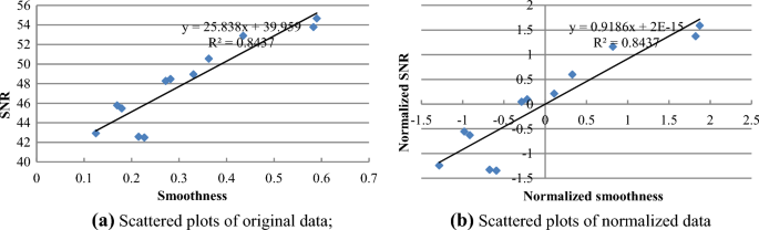
Scattered plots of pressure data. a Scattered plots of original data. b Scattered plots of normalized data
Figure 6a shows that the distribution of scattered points of original data has a strong linear correlation trend (R2 = 0.8437), which is table for PCA. At the same time, the general trend of data points after standardization has not changed, and the correlation coefficient of the two indicators is exactly the same with that before standardization, as shown in Fig. 6b. The regression model intercept of standardized data is approximately 0, and the slope is equal to the correlation coefficient.
-
Step 2 Calculate the correlation coefficient matrix or covariance matrix C for standardized data. These two matrixes are equal.
$$C = \left[ {\begin{array}{*{20}c} 1 & {0.91855} \\ {0.91855} & 1 \\ \end{array} } \right]$$(21) -
Step 3 The characteristic roots are calculated from the formula \(\left| {\lambda I - C} \right| = 0\). The results are λ1 = 1.91855, λ2 = 0.08145.
-
Step 4 Calculate the contribution rate Tj of the principal component and the cumulative variance contribution CTj based on the covariance matrix C and the characteristic roots, as shown in Table 1. It shows the percentage and cumulative percentage of the characteristic roots separately.
-
Step 5 Calculate the principal component load ρi, common factor variance Vi and variance contribution CVi by using Eq. (13), (14) and (15). The results are shown in Table 1.
-
Step 6 Determine the coefficients in different principal component linear combinations. By dividing the load ρi in Table 1 by extraction of the corresponding characteristic root, the coefficients in the linear combination of two principal components F1 and F2 can be obtained:
$$F_{1} = 0.7071x_{1} + 0.7071x_{2}$$(22)$$F_{2} = 0.7071x_{1} - 0.7071x_{2}$$(23) -
Step 7 Calculate the variance contribution rate of each principal component. The variance contribution rate can be regarded as the weight of different principal components, so it is equal to the weighted average of the coefficients in the linear combination of the principal components. Then construct the synthetic model:
$$F = 0.7071x_{1} + 0.6495x_{2}$$(24) -
Step 8 The coefficients of each principal component in the synthetic model are normalized. And the weights in the comprehensive evaluation index Tsrm for noise reduction are obtained at last. The weight of smoothness a is equal to 0. 5212, and the weight of SNR b is equal to 0.4788.
-
Step 9 The calculated comprehensive evaluation indexes Tsrm of various smoothing methods are shown in the first column on the right in Table 1.

The weights in the comprehensive evaluation index of noise reduction are provided in Table 1, and it can be seen that the moving window smoothing method excels for any given window width, so the moving window smoothing method is selected to deal with the pressure data in this paper.
Piecewise, multiple smoothing
The pressure datasets analyzed in this paper describe steady-state periods as well as several buildups and drawdowns. In this context, the smoothing should ensure the transient response is preserved. This is a problem when the width of the moving window is too large so that the transient process is easy to be ‘over-smoothed’ and some useful information lost.
That is why piecewise multiple smoothing is used to process these pressure data. The workflow is as follows: Firstly, the moving method with width = 5 is used for the first smoothing. The transient identification and separation are carried out on the basis of thus firstly smoothed data, and the pressure transients are identified and extracted. Then the remaining, steady-state data are smoothed for the second time and the third time using the window width = 15 and 30, respectively. This method not only protects the transient response and prevents the loss of useful information from it, but is also effective in removing the noise data during the steady pressure periods. The results for smoothness and SNR are shown in Fig. 7.

Processing results of different smoothing window width
It can be seen from Fig. 7 that the smoothness of the processed data decreases and the SNR increases slightly after the second smoothing (width = 15). However, after the third smoothing (width = 30), the smoothness decreases slightly, while the SNR decreases. Therefore, the reasonable way to process this pressure data is to use the moving smoothing method with twice-piecewise smoothing.
In addition, aiming at the problem that the moving smoothing method will cause the breakpoint forward, this paper improves the preferred smoothing method, that is, first find the breakpoints through transient identification; then divide the transient process according to the breakpoints; and smooth the data in each transient separately.
Wavelet threshold denoising and parameter optimization
From the previous data analysis, we can see that the temperature data in Fig. 4 are mixed with WGN, and so wavelet threshold denoising is table as efficient in removing WGN. Three important parameters of wavelet threshold denoising, namely wavelet function, threshold and decomposition level, are studied below and applied to the intelligent well temperature dataset.
Wavelet function
The denoising level of wavelet threshold methods is strongly dependent on the selected wavelet function, and a better denoising effect can be obtained by using the wavelet function with the shape resembling that of the transient response. According to this principle, the wavelet coefficients in Fig. 4 are compared with the waveforms of wavelet functions. Eventually, Db3 wavelet was selected as the wavelet function for temperature data processing, illustrated in Fig. 8.

Waveform of Db3 wavelet function
Selection of the decomposition level
The decomposition level is also important in the success of noise reduction. Generally, too many decomposition layers will lead to serious loss of signal information, reduction of SNR and increase of computational complexity. On the contrary, if the number of decomposition layers is too small, the effect of noise reduction is limited and so is the improvement of SNR.
The temperature data are processed by wavelet transform to get the detailed signal di and the approximate signal ai of each level, as shown in Fig. 9 (i = 1, 2…, 8). It can be seen from Fig. 9 that the noise data in the detailed signal of level 1–3 decrease with the increase of the decomposition scale. The noise in the detailed signal is too small to distinguish until it is decomposed to level 4. At the same time, the approximate signal of level 4 is consistent with the original signal. However, the approximate signal curve of level 5 and above has been distorted compared with the original data curve. Therefore, the optimal number of decomposition level for our temperature dataset is 4.

Approximate and detailed signal of wavelet transform applied to the temperature data. a Signals and approximations; b signals and details
Threshold
The methods of minimax and unbiased risk estimation criterion are conservative. When distribution of the noise in the high-frequency band signal is low, the two threshold estimation methods work better and can extract the weak signal. The fixed threshold and Heuristic threshold criterion methods are more effective at denoising, but can also remove the useful high-frequency signals mistaken for noise.
Selection of the optimal combination of noise reduction methods
The wavelet analysis tools from the MATLAB platform were applied to reduce the noise in the temperature dataset. As explained above, the db3 wavelet function and the decomposition level 4 were selected. The four-threshold criteria are adopted and processed by the soft threshold method. The results are shown in Fig. 10.

Wavelet denoising results of temperature data with different threshold criteria a fixed soft; b Heuristic sure-soft; c minimax soft; d rigorous sure-soft
The results of different threshold methods have different smoothness, as shown in Fig. 10. The results of fixed threshold denoising have the best smoothness and the best white noise removal, as shown in Fig. 10a, but its SNR is the lowest (see Table 2). By contrast, the denoised data obtained by rigorous sure threshold have the worst smoothness but the highest SNR, as shown in Fig. 10d and Table 2. Therefore, it is difficult to determine directly which denoising combination is most table for the temperature data by the smoothness and SNR in Table 2.
So we use PCA to analyze the four sets of noise reduction method results and determine the weights in the comprehensive evaluation index. Then, the denoising combination is selected according to the value of the comprehensive evaluation index. The parameter values of PCA and the final weights are shown in Table 2. The fixed threshold method has the highest value of comprehensive evaluation index. Therefore, the combination of db3 wavelet function, 4-layer wavelet decomposition and the fixed threshold method is the most table combination for the temperature data set. These conclusions will be further confirmed in the next section.
Results and analysis
Case 1
The data for this case are the transient annulus pressure and temperature measurement from the third zone in a three zone intelligent well, where the third zone is the deepest and the first zone is the shallowest. Movement of the surface choke or any of the zonal control valves resulted in transient events, and any of these events can be selected for the analysis.
The processed temperature and pressure data, as shown in Fig. 11, can be used for TTA and PTA. According to the requirements of data analysis, three pressure transients and corresponding temperature data, highlighted in the three black rectangular boxes I, II, III in Fig. 11, are selected from the data set to carry out TTA with the input from pressure. Transient event I is due to the closing of the surface choke which results in a pressure buildup in all the open zones, zone 3 inclusive, while event II is due to the closing of the ICV (interval control valve) of the third zone resulting in a pressure buildup in that zone. Finally, event III is due to the opening of the ICV-1 which leads to a pressure drawdown in zone one, and a corresponding pressure buildup in zone 3. Pressure and temperature data in the transients are extracted and analyzed separately, as shown in Fig. 12, 13 and 14.

Denoised pressure and temperature data of Case 1

TTA of transient I: ε′ = dT/dP = 0.8/30 = 0.0267 C/psi

TTA of transient II:ε′ = dT/dP = 0.48/20 = 0.024 C/psi

TTA of transient III: ε′ = dT/dP = 0.13/5 = 0.026 C/psi
The slope ratio of the temperature and pressure curves in each transient is calculated following the same logic as described in Sect. 2.5 above or for calculating the Joule–Thomson coefficient as described in (Muradov 2017; Onur 2016). The results show that the three values are close. This is physical because the slopes ratio coefficient of the fluid for the given transient period remains the same during the period where the fluid composition does not change. The fact that the selected denoising method showed this consistency confirms that it is table for the PDG data of this kind and for the subsequent TTA.
Case 2
The PDG data of Case 2 are from Zone 1 of an intelligent well with three production layers. The selected pressure buildup transients of Zone 1 are caused by the gradually opening of ICV2, while the ICV1 remained open completely during this period.
The same methods, illustrated above, are used to process the data. The results are as shown in Fig. 15. The annulus pressure reveals periods when the ICVs are cycled (i.e., gradually opened) regularly during production. So the data measured during such cycling can be used for PTA and TTA. Five transients are extracted from this data set, and the ratio of temperature and pressure slopes is calculated, as shown in Figs. 16, 17, 18, 19, and 20.

Denoised pressure and temperature data of Case 2

TTA of transient I: ε′ = dT/dP = 0.011/0.02 = 0.55 C/bar

TTA of transient II: ε′ = dT/dP = 0.011/0.02 = 0.55 C/bar

TTA of transient III: ε′ = dT/dP = 0.023/0.04 = 0.575 C/bar

TTA of transient IV: ε′ = dT/dP = 0.01/0.018 = 0.556 C/bar

TTA of transient V: ε′ = dT/dP = 0.024/0.04 = 0.6 C/bar
The results show that the values are approximately equal, which means the slopes ratio coefficient ε’ is identified as constant during this period, which is physical because the fluid properties in this well did not change during the testing. This again confirms the effectiveness of the processing methods proposed in this paper.
Example use of denoised data in transient analysis
We have deliberately omitted in-depth use of pressure and/or temperature transient analysis methods in this paper. The beauty of the verification method we have chosen in this paper, i.e., the one based on the consistency of the estimated pressure/temperature slopes ratio coefficient ε′ (see Eq. 20) using both the correctly denoised pressure and the correctly denoised temperature signals, is that it completely rests on the fundamental temperature solution (Eq. 20) and is independent of any further interpretation models and assumptions. The ε′ consistency (in multiple transient events in a given well) observed in this paper confirms the stability of the developed signal denoising methodology which was the very objective of this paper.
As an illustration, to put this into context and briefly show how this may further aid a potential pressure and temperature transient analysis (PTTA), let us consider Case 2 a bit further. The PTTA principles and assumptions applicable to the wells used in this paper will take another publication to properly describe. Fortunately, the ‘Case 2′ well PTTA on the very dataset used in this paper was already described and applied in (Muradov et al. 2017). We refer the readers to that publication for more details. In short, our paper’s results translate to the (Muradov et al. 2017) work as follows:
Muradov et al. (2017) have described the field, the well completion, the well control and testing sequence, as well as the temperature transient physics and solutions table. They have also compared the traditional PTA results (as obtained by the field operator in SAPHIR™) with the ones estimated using late-time IARF TTA solution. The data were not properly denoised in that study.
For the dataset analyzed in both our and (Muradov et al. 2017) papers, referred to as ‘Case 2 Zone 1′ and ‘Well A Zone 1′ dataset, respectively, the traditional PTA analysis estimated the zone’s KH (i.e., the permeability thickness product) to be ~ 71,000 mD ft (see Table 1 in Muradov et al. (2017)). This KH value has been found by the field operator from multiple PBUs and is considered as a reliable reference point. The ‘noisy’ TTA model estimated this KH at ~ 75,000 mD ft (see Table 2 in Muradov et al. (2017)).
The coefficient ε′ estimated from the raw, noisy data (i.e., directly from the ones plotted in Fig. 3b top and 4b top) is around 0.6 °C/bar for the time periods chosen in this work. It is hard to estimate it any better due to noise. The same coefficient estimated from the denoised data in this work (see the titles to Figs. 17,18, 19 and 20) is much clearer and is on average 0.566 °C/bar. This means the TTA-estimated, ‘noisy’ KH product in (Muradov et al. 2017) should be corrected by 0.566/0.600 = 0.94 to eliminate the effect of the pressure and temperature measurements’ noise. Correcting the ‘noisy’ KH as 0.94 × 75,000 mD ft gives 70,500 mD ft, bringing this KH estimate closer to the reference, PTA-estimated value of 71,000 mD ft.
This increases confidence in the TTA results, proving that the key parameters like KH can be well estimated using the temperature transient data alone (e.g., where the pressure signal is not measured, is unreliable or is masked by wellbore storage effects) provided the data have been processed correctly, preferably following the denoising approach developed in this paper.
We hope this example underlines the value of the universal, user-independent denoising framework developed for and tested on downhole P and T transient data in this paper.
Conclusion
Temperature transient analysis in wells has been paid much attention during the past two decades. Tens of brand new TTA models, solutions and applications for very diverse well production and fluid conditions have been published by many key, transient analysis champions worldwide: from Stanford to Heriot-Watt, from Chevron to CNOOC.
It has been widely accepted that since the temperature changes used in TTA are very small (e.g., for oil well they are typically on the scale of 0.1 °C), TTA is only possible when high-precision temperature sensors are installed downhole. Such sensors themselves have the typical resolution of around 0.02 °C. Given that this useful signal value is not very different from the sensor resolution, it is very important to apply the right data cleansing and denoising approach to the temperature data to turn the data ‘cloud’ into a reliable, ‘analyzable’ series. It is tempting to blindly use the same data denoising algorithms for temperature as for pressure. This paper is the first to rigorously and systematically check and establish which particular methods would be applicable to pressure and which ones to temperature, how to select from them, how to tune the denoising algorithm based on the data alone (e.g., without arbitrarily set thresholds) and how to make sure the selected approach retains the physics expected by the PTTA.
First in this paper, the denoising method was chosen according to the characteristics of detail signals of the wavelet transform. For instance, wavelet threshold denoising methods are used to remove white noise and WGN, while data smoothing is table for removing impulse noise. We have shown that the pressure data are dominated by the impulse noise, while the temperature data had mostly white noise in it and have proposed the optimal demising algorithms for each.
Next, we introduced the new comprehensive evaluation index effective to select optimal combination of noise reduction, so that noise and useful signal can be separated quickly and accurately. The SNR and smoothness were taken as the evaluation indexes of the noise reduction results, and the weights of the two indexes are determined by PCA, which ensures the noise reduction results meet the requirements of data processing and data analysis at the same time. The PCA weights are independent of the user input and are determined by the data alone.
Finally, the improved processing method was applied to the datasets from two intelligent, oil production wells. This showed TTA analysis consistency for multiple transients confirming that the improved processing methods are effective. We have also illustrated how the denoised TTA-estimated KH product is more accurate compared to the ‘noisy’ one estimated in a previous publication.
The denoising methodology developed and verified in this paper is recommended for in-well PDG data to improve the accuracy and reliability of the data in TTA and PTA.
Abbreviations
- PDG:
-
Permanent downhole gauge
- WGN:
-
White Gaussian noise
- SNR:
-
Signal-to-noise ratio
- PCA:
-
Principal component analysis
- TTA:
-
Temperature transient analysis
- ICV:
-
Inflow control valve
- PSNR:
-
Power signal-to-noise ratio
- RMSE:
-
Root-mean-square error
- h :
-
Reservoir thickness
- k :
-
Permeability
- K :
-
Thermal conductivity
- L :
-
Distance from well to reservoir boundary
- p :
-
Pressure
- Q :
-
Volumetric flow rate (surface)
- ε :
-
Joule–Thomson coefficient
- q :
-
Flow rate (downhole)
- S :
-
Saturation
- T :
-
Temperature
- v :
-
Velocity
- η :
-
Thermal expansion coefficient
- μ :
-
Dynamic viscosity
- \(C_{\rm P}\) :
-
Mass heat capacity at constant pressure
- \({ }\emptyset\) :
-
Porosity
- \(C_{f}\) :
-
Reservoir rock compressibility
- \(\beta\) :
-
Volumetric thermal expansivity
- \(v\) :
-
Velocity vector
- \(C_{pf}\) :
-
Heat capacity of formation rock
- \(\rho\) :
-
Density
- T:
-
Tubing
- R:
-
Radial direction
- F:
-
Formation
References
Athichanagorn S (1999) Development of an interpretation methodology for long-term pressure data from permanent downhole gauges. Stanford University, Palo Alto, California
Athichanagorn S,Horne RN1999). Processing and interpretation of long term data from permanent down hole pressure gauges. Paper SPE56419 presented at the1999 SPE annual technical conference and exhibition, Houston, Texas, 3–6 Oct
Bellarby J (2009) Well completion design. Elsevier, Amsterdam
Cai T, Zhu J (2006) Adaptive selection of optimal decomposition level in threshold de-noising algorithm based on wavelet. Control Decis 21(2):217–220
Chang SG, Yu B (2000) Adaptive wavelet thresholding for image denoising and compression. IEEE Trans Image Process 9(9):1532–1546
Chang F, Hong W et al (2010) Research on wavelet denoising for pulse signal based on improved wavelet thresholding. In Jun Jiang, Jian Guo, Weihua Fan et al (eds) first international conference on pervasive computing, signal processing and applications, p 564–567 2010. An improved adaptive wavelet denoising method based on neighboring coefficients. Proceedings of the 8th world congress on intelligent control and automation, Jinan, China, p 2894–2898, 6–9July
Dada A, Muradov K, Davies D (2017) Temperature transient analysis models and workflows for vertical dry gas wells. J Nat Gas Sci Eng 45:207–229
Donoho DL, Johnstone IM (1994) Ideal spatial adaptation by wavelet shrinkage. Biometrika 81(3):425–455
Donoho DL, Johnstone IM (1995) Adapting to unknown smoothness via wavelet shrinkage. J Am Stat Assoc 90(432):1200–1224
Donoho DL, Johnstone IM (1998) Minimax estimation via wavelet shrinkage. Ann of Stat 26(3):879–921
Donoho DL (1995) De-noising by soft-thresholding. IEEE Trans Inform Theory41(3):6l2–627
Duru O, Horne R (2010) Modeling reservoir temperature transients and reservoir-parameter estimation constrained to the model. SPE Reserv Eval Eng 13(6):873–883
Duru O, Horne R. (2008) Modeling reservoir temperature transients and matching to permanent downhole gauge data for reservoir parameter estimation. In Proceedings of SPE annual technical conference and exhibition. society of petroleum engineers.
Huimin C, Ruimei Z, Yanli H (2012) Improved threshold denoising method based on wavelet transform international conference on medical physics and biomedical engineering. Phys Procedia 33:1354–1359
Jenkal W, Latif R et al (2016) An efficient algorithm of ECG signal denoising using the adaptive dual threshold filter and the discrete wavelet transform. Biocybern biomed eng 36:499–508
Khong CK (2001) Permanent downhole gauge data interpretation. Stanford University, Palo Alto, California
Kong LJ (2014) Super learning manual of matlab wavelet analysis. Posts & Telecom Press, Beijing
MF Silva Junior, K Muradov, MS Carvalho (2012) Modeling and analysis of temperature transients caused by step-like change of downhole flow control device flow area. Paper SPE153530 presented at the SPE Latin American and caribbean petroleum engineering conference, Mexico City, 16–18 April
Madhur S, Anderson CL, Freed JH (2016) A new wavelet denoising method for selecting decomposition levels and noise thresholds. IEEE Access 4:3862–3877
Madhur S, Bhavani HB (2015) A novel algorithm for denoising of simulated partial discharge signals using adaptive wavelet thresholding methods. IEEE Sponsored 2nd international conference on electronics and communication system (ICECS 2015), 1596–1602
Mao Y, Zeidouni M (2018) Accounting for fluid-property variations in temperature-transient analysis. SPE J 23(03):868–884
Mao Y, Zeidouni M (2017) Analytical solutions for temperature transient analysis and near wellbore damaged zone characterization. In SPE reservoir characterisation and simulation conference and exhibition. society of petroleum engineers
Muradov K, Davies D (2017). Transient pressure and temperature interpretation in intelligent well of the golden eagle field. Paper SPE185817 presented at the SPE Europec featured at 79th EAGE Conference and Exhibition, Paris, France, 12–15 June
NI (2011) Overview of fiber optic sensing technologies. Available at: https://www.ni.com/white-paper/12953/en/. Accessed Nov 8 2017
Olsen S, Nordtvedt JE, Epsis, 2005. Improved wavelet filtering and compression of production data. PaperSPE96800presented at the Offshore Europe, Aberdeen, Scotland, 6–9 Sep 2005
Onur, M(2017) Modeling and interpretation of the bottomhole temperature transient data. PaperSPE185586 presented at the SPE Latin American and caribbean petroleum engineering conference, Buenos Aires, Argentina, 18–19 May
Onur M, Çinar M (2016) Temperature transient analysis of slightly compressible, single-phase reservoirs. In SPE Europec featured at 78th EAGE conference and exhibition. Society of petroleum engineers
Ouyang LB, Kikani J (2002) Improving permanent down hole gauge(PDG) data processing via wavelet analysis. PaperSPE78290presented at the SPE 13th European petroleum conference, Scotland, 29–31 Oct
Rakshit M, Das S (2018) An efficient ECG denoising methodology using empirical mode decomposition and adaptive switching mean filter. Biomed Signal Process Control 40:140–148
Ramazanov A. et al (2010) Thermal modeling for characterization of near wellbore zone and zonal allocation. In SPE Russian oil and gas conference and exhibition. Society of petroleum engineers
Sui W et al, (2008) Model for transient temperature and pressure behavior in commingled vertical wells. In SPE Russian oil and gas technical conference and exhibition. Society of petroleum engineers
van Gisbergen SJCHM, Vandeweijer AAH (1999) Reliability analysis of permanent downhole monitoring systems. In offshore technology conference. Offshore technology conference
Viberti D, Verga F, DelboscoP2005) An improved treatment of long-term pressure data for capturing information. Paper SPE96895 presented at the 2005 SPE annual technical conference and exhibition, Dallas, Texas, 9–12 Oct
Viberti D, Verga F, Delbosco P (2005) An improved treatment of long-term pressure data for capturing information. Paper presented at the 2005 SPE annual technical conference and exhibition, SPE96895, Dallas, Texas 9–12 Oct 2005
Xiong P, Wang H et al (2018) ECG signal enhancement based on improved denoising auto-encoder. Eng Appl Artif Intell 52:194–202
Yankui S (2005) Wavelet analysis and application. Mechanical Industry Press, Beijing
Yoshioka K, Zhu D, Hill A (2006) Detection of water or gas entries in horizontal wells from temperature profiles. SPE Europec/EAGE annual conference and exhibition, Vienna, 12–15 June
Zhang X, Desai M (1998) Adaptive denoising based on sure risk. Publ IEEE Signal Process Lett 5(10):265–267
Zhang B, Xiong J, Zhang N (2016) Improved method of processing downhole pressure data on intelligent wells. J Nat Gas Sci Eng 34:1115–1126
Zhao Q, Dai W (2015) A Wavelet Denoising Method of New Adjustable Threshold. Proceedings of ICCT2015,684–688
Acknowledgements
We thank the sponsors of the “Value from Advance Wells” Joint Industry Project at Heriot-Watt University, Edinburgh, UK, for their financial support and data provision. We also thank the Education Fund for Young Teachers of Xi'an Shiyou University, China, for their financial support.
Funding
Supported By Open Fund (PLC2020033) of State Key Laboratory of Oil and Gas Reservoir Geology and Exploitation (Chengdu University of Technology).
Author information
Authors and Affiliations
Corresponding author
Additional information
Publisher's Note
Springer Nature remains neutral with regard to jurisdictional claims in published maps and institutional affiliations.
Rights and permissions
Open Access This article is licensed under a Creative Commons Attribution 4.0 International License, which permits use, sharing, adaptation, distribution and reproduction in any medium or format, as long as you give appropriate credit to the original author(s) and the source, provide a link to the Creative Commons licence, and indicate if changes were made. The images or other third party material in this article are included in the article's Creative Commons licence, unless indicated otherwise in a credit line to the material. If material is not included in the article's Creative Commons licence and your intended use is not permitted by statutory regulation or exceeds the permitted use, you will need to obtain permission directly from the copyright holder. To view a copy of this licence, visit http://creativecommons.org/licenses/by/4.0/.
About this article

Cite this article
Zhang, B., Muradov, K. & Dada, A. Principal component analysis-assisted selection of optimal denoising method for oil well transient data. J Petrol Explor Prod Technol 11, 509–530 (2021). https://doi.org/10.1007/s13202-020-01010-3
Received:
Accepted:
Published:
Issue Date:
DOI: https://doi.org/10.1007/s13202-020-01010-3