
Abstract
The tight reservoirs in Dagang Oilfield are deep in burial depth and complex in lithology, and the brittleness evaluation methods commonly used at home and abroad are not accurate enough to effectively guide the design of fracturing. As a result, the fracturing in the early days was low in success rate and not ideal in effect. In this study, from the perspective of breaking energy theory, based on a large number of core experiments, the factors affecting rock failure morphology have been analysed by using the breaking energy theory, and a brittleness evaluation method more suitable for the physical properties of tight reservoirs in Dagang Oilfield has been worked out. The results show that the main parameters affecting brittleness of tight reservoirs in Dagang Oilfield are Young’s modulus, dilatancy angle and peak strain. The correlation coefficient between the brittle index from the new method based on breaking energy theory and rock failure complexity increases to 0.789 compared with 0.329 of the brittle index from Rickman’s evaluation method. The new method solves the problem that previous brittleness index models at home and abroad are not suitable for tight reservoirs in Dagang Oilfield, and provides a theoretical basis for evaluating the fracability of tight reservoirs and improving fracturing effect in Dagang Oilfield.
The tight oil and gas reservoirs in Dagang Oilfield include tight reservoirs in the second member of the Kongdian Formation (Ek2) in Cangdong sag and the lower section of the first member of the Shahejie Formation (EsL1) in Qikou sag. They have a porosity range from 5.09 to 10.51% and permeability range from 0.44 to 6.84 × 10⁻³ μm2 and shale content range from 11.46 to 41.5%, of which reservoirs with permeability of less than 1 × 10⁻³ μm2 account for 30% (Pu et al. 2016). The reservoirs have the characteristics of large burial depth, well-developed natural fractures, complex lithologies and poor physical properties. The rock brittleness, natural fracture characteristics and geostress state of tight reservoirs in Dagang Oilfield have the foundation of forming complex fractures. However, whether complex fractures can be formed and the mechanism controlling the formation of complex fractures are not clear. The calculation methods of rock brittleness index currently available at home and abroad are not suitable for Dagang tight reservoirs. Consequently, fracturing before was low in success rate and not ideal in effect. The process of rock failure is the process of energy absorption and release. The energy characteristic is the essential feature of rock failure. The lower the energy consumed by rock failure, the greater the rock brittleness will be. Therefore, the rock failure characteristics have been analysed from the view point of energy, and the brittleness evaluation method has been established based on the relationship between fracture energy and mechanical parameters and mineral composition in this study.
Calculation of breaking energy
According to the theory of fault mechanics, the energy consumed by crack propagation per unit area is breaking energy. Firstly, the stress–strain relationship considering dilatancy was established, then the energy of rock failure was calculated, to compare and analyse the energy dissipation (Sneddon and Elliot 1946) characteristics of tensional failure and shear failure, and the breaking energy was calculated according to the size of rock failure surface.
A method for calculating breaking energy of rock failure
The surface energy per unit area of a crack is assumed to be R. According to Griffith’s energy criterion, the crack propagation process needs to satisfy:
where G is the driving force of crack propagation, i.e. the dynamic force provided by the system is greater than or equal to the resistance of crack propagation per unit area. If the potential energy of the whole system is assumed to be \(\prod\), the energy consumed by the crack to propagate the area \(\Delta S_{\text{c}}\) is as follows:
According to the energy conservation theory, the consumption of energy is equivalent to the decrease in the potential energy of the system (\(- \Delta \prod\)), i.e.:
G is the energy release rate of the system, also known as breaking energy.
According to the theory of deformation potential energy of elastomer, assuming that the elastomer keeps balance during the process of loading, the decreases in external force potential energy, that is, the work done by the external force is completely transformed into deformation potential energy and stored in the interior of the elastomer. Deformation potential energy can be calculated by work done by stress in its strain direction. Its magnitude is the superposition of each stress component, and the strain energy per unit volume can be expressed in terms of strain energy density.
From the generalized Hooke’s law:
If the strain energy produced by circumferential deformation is neglected, the releasable strain energy (Ue) can be calculated by the following formula.
According to the theory of brittle fracture mechanics, the rock breaks when the elastic strain energy release rate accumulated in the rock is equal to the energy required to produce the surface of the fracture body per unit area (Palmer 1991). If the crack surface area generated by rock failure is assumed to be S, the breaking energy of rock failure is:
Under triaxial compression, the energy absorbed by rock deformation and failure is the sum of the releasable strain energy (Ue) stored in rock and dissipated energy of plastic deformation of rock sample (Ud). The total energy absorbed by the rock sample can be expressed as:
The dissipation energy in plastic deformation process of rock can be expressed as follows:
The dissipation energy of rock can be expressed by the stress–strain relationship of the rock:
The stress–strain relationship can also be obtained from triaxial compression test data, and then, the energy of rock deformation and failure can be calculated. The breaking energy of rock failure can be calculated by combining the size of rock failure surface (Nolte and Smith 1981).
A method for calculating crack area
After this experiment, the fracture area of failed rock sample needed to be calculated and counted. For rock samples after triaxial compression test, macroscopic visible fractures can be better identified. According to the rupture angle of fracture surface in the rock sample, the area of fracture surface can be calculated (Hossain et al. 2000).
- 1.
When the rupture angle is equal to 0 (as (a) in Fig. 1), the formula for calculating the fracture area is:
Fig. 1 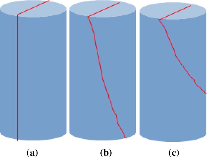
Several failure forms of fractures with different rupture angles

where H—rock sample height (m); \(C_{i}\)—length of the ith fracture along strike direction (m).
- 2.
When the rupture angle is equal to 0 and less than \(\beta\) (as (b) in Fig. 1), the formula for calculating the fracture area is:
where \(C_{\text{up}}\) and \(C_{\text{down}}\)—length of upper and lower surface along strike direction (m).
- 3.
When the rupture angle is larger than \(\beta\) and less than 90°(as (c) in Fig. 1), the formula for calculating the fracture area is:
where D—core diameter (m); \(\alpha_{i}\)—rupture angle of the fracture (Fig. 2).

Sketch graphs of fracture parameters
According to the above method, the total area of fractures in the fractured rock sample can be calculated, that is, the sum of the surface area of all fractures:
Laboratory experiment of rock mechanics
Experiment of rock mechanics
In order to study the effect of mechanical parameters on fracture morphology, triaxial rock mechanics experiments were conducted first. In total, 20 groups of core samples were taken from K2 member. The core samples about 50 mm long and 25.4 mm in diameter were drilled with coring bit. The end faces of them were processed with lathe to make them parallel. The end faces and perimeter of the samples were smoothed by a grinder (Fig. 3). The mechanical properties of rock samples were tested, and triaxial rock mechanics tests were carried out. The results are shown in Table 1.

Photographs of core samples used in triaxial rock mechanics tests
The crack area caused by rock failure was obtained based on the triaxial compression test results. According to the energy consumed by the failure of each rock sample, the breaking energy of rock failure was calculated, to analyse the relationship between the parameters and breaking energy.
Relationship between breaking energy and complexity of rock failure
Figure 4 shows the relationship between breaking energy and complexity of rock failure. It can be seen from this figure that breaking energy decreases with the increase in complexity of rock failure; in other words, they have a good correlation. This indicates that the greater the degree of rock fragmentation, the smaller the energy needed to produce a unit crack area will be.

Relationship between breaking energy and complexity factor of rock failure
Study on the relationship between breaking energy and mechanical parameters
Relationships between breaking energy and Young’s modulus and Poisson’s ratio
Figures 5 and 6 show the relationships between breaking energy of rock and Young’s modulus and Poisson’s ratio. It can be seen from the graphs that the breaking energy of rock is negatively correlated with Young’s modulus and positively correlated with Poisson’s ratio. The larger the Young’s modulus, and the smaller the Poisson’s ratio, the smaller the breaking energy of rock is. Of them, the correlation between breaking energy and Young’s modulus is much greater than Poisson’s ratio, while the correlation between Poisson’s ratio and breaking energy is not significant.

Relationship between breaking energy and Young’s modulus

Relationship between breaking energy and Poisson’s ratio
Relationship between breaking energy and mineral contents
Figures 7, 8 and 9 show the relationships between breaking energy and quartz content, silicate content and carbonate content, respectively. It can be seen from the figures that the correlation between breaking energy and the mineral contents is not significant.

Relationship between breaking energy and quartz content

Relationship between breaking energy and silicate content

Relationship between breaking energy and carbonate content
Relationships between breaking energy and stress and strain
Figures 10 and 11 show the relationship between breaking energy and peak strain and peak stress. It can be seen from the figures that the larger the peak strain is, the greater the breaking energy of rock failure is, and the correlation between them is good. But there is little correlation between breaking energy and peak stress.

Relationship between breaking energy and peak strain

Relationship between breaking energy and peak stress
Relationship between breaking energy and rock dilatancy
Figure 12 shows the relationship between breaking energy and dilatancy angle. It can be seen from the graph that the larger the dilatancy angle, the smaller the breaking energy of rock failure is. They are quite closely correlated.

Relationship between breaking energy and dilatancy angle
From the above analysis results, it is found that there is a good correlation between rock breaking energy and rock fault complexity factor, showing the consistency between failure morphology and breaking energy, and that the proposed method can better reflect the energy characteristics of rock failure. From the energy analysis, it can be seen that the shear failure mode consumes more energy, produces smaller crack area and has larger breaking energy; while the tensile failure mode consumes less energy, produces more cracks and larger crack area, so its breaking energy is smaller. It can also be seen from the results of correlation analysis of various factors with breaking energy that Young’s modulus, peak strain and dilatancy angle can better reflect the characteristics of rock breaking energy, while mineral composition, Poisson’s ratio and peak stress of rock have little correlation with breaking energy.
The influencing factors of breaking energy were analysed by calculating model of breaking energy of rock failure. The correlation coefficients between breaking energy and Young’s modulus, dilation angle and peak strain are 0.38, 0.56 and 0.59, respectively, while Poisson’s ratio and mineral composition have little correlation with breaking energy. Meanwhile, it is found that the Ek2 tight sandstone is complex in lithology and stress state, and its brittleness has little correlation with mineral composition, so the evaluation method of shale mineral brittleness is not fully applicable.
Mathematical model for brittleness evaluation
Young’s modulus, dilatancy angle and peak strain can, respectively, reflect the ability to resist deformation, deformation rate and deformation size of the rock and can better describe the brittle characteristics of the rock, while mineral composition and Poisson’s ratio, etc., cannot accurately describe the brittle characteristics of the rock. Meanwhile, the three parameters, Young’s modulus, dilation angle and peak strain, all reflect the characteristics of different stages on the stress–strain curve, and there is no repeatability of characteristics they describe. Their linear combination is simple and practical. By giving the parameters corresponding weights, the brittleness evaluation method can be established, which can reflect the characteristics of the whole stress–strain curve.
Therefore, the brittleness evaluation method suitable for tight sandstone is established as follows:
where \(B_{I}\)—brittleness index; \(E_{n}\), \(\psi_{n}\) and \(\varepsilon_{pn}\)—normalized Young’s modulus, dilatancy angle and peak strain; W1, W2 and W3—weight coefficients of the parameters, \(W_{1} + W_{2} + W_{3} = 1\).
The calculation equations of \(E_{n}\), \(\psi_{n}\) and \(\varepsilon_{pn}\) are:
where the variables with max and min subscripts are the maximum and minimum values of the parameters, respectively.
The physical meaning of the model is to calculate the brittleness index based on Young’s modulus, dilatancy angle and peak strain. Because we have found that these factors are the most obvious parameters through the result of experiments, we cannot get quantitative relationship between brittleness index and parameters just rely on our experiments data. Grey relational method can help us to clear the quantitative relationship between brittleness index and every parameter. The grey relational theory was used to calculate the weight coefficients. This theory put forward the concept of grey relational degree analysis for each subsystem, and the numerical relationships between subsystems in the system are sought through certain methods. For the factors between two systems, the correlation degree is defined as a measure of the size of the correlation that changes with time or with different objects. If two factors change in similar trends, they have higher correlation degree; conversely, it is lower. At present, correlation degree analysis has been widely applied to various fields of scientific research. It mainly includes the following steps:
- 1.
Determine subseries and reference series
The factors affecting brittleness are considered as subseries, and the expression of subseries is as follows:
The breaking energy of rock failure is taken as a reference series, and its expression is as follows:
- 2.
Calculate utility function
In order to eliminate the unit interference of physical quantities, the data were processed by normalization method. According to the previous analysis results, the three parameters related to breaking energy are Young’s modulus, dilatancy angle and peak strain. According to the differences of the previous statistical results, the following two methods were used to process the data.
The utility function of the index that is better when bigger can be calculated by:
The utility function of the index that is better when smaller can be calculated by:
where \(\left( {r_{ij} } \right)_{{\min} }\) and \(\left( {r_{ij} } \right)_{{\max} }\)—minimum and maximum value of a sample
Then the function matrix can be got by:
- 3.
Calculate correlation coefficient
where
\(\rho \in \left( {0, + \infty } \right)\) is resolution coefficient. The smaller \(\rho\) indicates higher resolution. \(\rho\) is between [0,1].
- 4.
Calculate correlation degree
The correlation coefficient and correlation degree of subsequences are both greater than 0, and the correlation degree of subsequences should be the average of each correlation coefficient, so it can be obtained as:
- 5.
Calculate weight coefficient
All parameters have different influences on brittleness. In order to compare the influences of the parameters, the weight coefficient of a factor can be calculated by the proportion of the correlation degree of the factor to the total correlation degree.
For breaking energy and peak strain, we adopted the utility function that is better when smaller; for Young’s modulus and dilatancy angle, we adopted the utility function that is better when bigger. The processing results are shown in Table 2.
Based on the above data, the weight coefficient of each parameter is calculated as follows: 0.262 for Young’s modulus, 0.353 for dilatancy angle and 0.385 for peak strain.
Therefore, the brittleness evaluation method suitable for tight sandstone is established as follows:
where \(B_{I}\)—brittleness index; \(E_{n}\), \(\psi_{n}\) and \(\varepsilon_{pn}\)—normalized Young’s modulus, dilatancy angle and peak strain.
According to the above weighting coefficients, the brittleness indexes of 42 rock samples selected in this study were calculated and compared with the brittleness indexes calculated with Rickman method (Rickman et al. 2008). And the relationship between the brittleness index and the complexity of rock failure was plotted. Figure 13 shows the relationships between the proposed brittleness index, Rickman’s brittleness index and the complexity coefficient of rock failure. It can be seen that the proposed model has a higher correlation with the complexity coefficient of rock failure, which indicates that the results of comprehensive consideration of the three factors have a good combination effect. The comparison with results from Rickman’s method shows that the proposed model can better reflect the complexity of rock failure.

Relationship between brittleness index and complexity of rock failure
From the relationship between brittleness index and complexity factor of rock failure, we know that the complex is formed when the brittleness index is more than 0.4 if the value of brittleness index based on our new model less than 0.4. It is hard to form complex fracture. We need to consider more technical technology to form complex fracture in the process of our fracture design (Fig. 14).

Relationship between brittleness index and complexity factor of rock failure
Field application
The new brittleness index model was tested in Well G1. Ek2 in Well G1 is tight oil reservoir, with 4135.5–4164.8 m fractured and 29.3-m-thick oil layer. The fracture net index of the fractured interval in this well was calculated at 0.44, which indicates that complex fractures are likely to form to make up network by fracturing. The fracturing was done at the injection rate of 10–12 m3/min and used a total of 924.2 m3 fracturing fluid and 71.8 m3 proppant. It produced 0.54 m3 liquid daily by measuring liquid level before fracturing and 32.6 m3 of oil per day with 3-mm nozzle after fracturing. The results of fracture monitoring show that a fracture network of 419 metres long, 124 metres wide and 71 metres high has been formed. The main fractures strike northeast–southwest, and also there were branching fractures striking northwest–southwest coming up. The evaluation results of the new brittleness index model are consistent with field fracture monitoring, which provides an effective basis for volume fracturing of Dagang tight oil reservoirs (Fig. 15).

Top view (left) and side view (right) of fractures
Conclusions and suggestions
For the Ek2 tight reservoirs in Dagang Oilfield, rock breaking energy has a correlation coefficient with Young’s modulus, dilatancy angle and peak strain of 0.38, 0.56 and 0.59, respectively, but has little correlation with Poisson’s ratio and mineral composition.
Compared with the brittleness index from Rickman’s evaluation method with a correlation coefficient of 0.329 with rock failure complexity, the correlation coefficient between the brittleness index calculated with the newly proposed method and rock failure complexity increases to 0.789, solving the problem that previous brittleness index models at home and abroad are not suitable for tight oil reservoirs in Dagang Oilfield. When the mechanical brittleness index is greater than 0.4, the fracture morphology of rock is complex.
The field application results show that the judgement of whether network fractures can be formed or not with the new brittleness index model is consistent with the monitoring results of fracturing, proving it can provide a basis for volume fracturing of Dagang tight oil reservoirs.
References
Hossain MM, Rahman MK, Rahman SS (2000) Hydraulic fracture initiation and propagation: roles of wellbore trajectory, perforation and stress regimes. J Petrol Sci Eng 27(3):129–149
Nolte KG, Smith MB (1981) Interpretation of fracturing pressures. J Petrol Technol 33(9):1767–1775
Palmer ID (1991) Induced stresses due to propped hydraulic fracture in coal bed methane wells. In: SPE25861
Pu X, Zhou L, Han W, Zhou J, Wang W, Zhang W, Chen S, Shi Z, Liu S (2016) Geologic features of fine-grained facies sedimentation and tight oil exploration: A case from the Second Member of Paleogene Kongdian Formation of Cangdong sag, Bohai Bay basin. Pet Explor Dev 43(1):26–35
Rickman R, Mullen MJ, Petre JE, Grieser WV, Kundert D (2008) A practical use of shale petrophysics for stimulation design optimization: all shale plays are not clones of the Barnett shale. In: Society of Petroleum Engineers annual technical conference and exhibition, Denver, 21–24 Sept 2008
Sneddon IN, Elliot HA (1946) The opening of a Griffith crack under internal pressure. Quart Appl Math 4(3):262–267
Author information
Authors and Affiliations
Corresponding author
Additional information
Publisher's Note
Springer Nature remains neutral with regard to jurisdictional claims in published maps and institutional affiliations.
Rights and permissions
Open Access This article is licensed under a Creative Commons Attribution 4.0 International License, which permits use, sharing, adaptation, distribution and reproduction in any medium or format, as long as you give appropriate credit to the original author(s) and the source, provide a link to the Creative Commons licence, and indicate if changes were made. The images or other third party material in this article are included in the article's Creative Commons licence, unless indicated otherwise in a credit line to the material. If material is not included in the article's Creative Commons licence and your intended use is not permitted by statutory regulation or exceeds the permitted use, you will need to obtain permission directly from the copyright holder. To view a copy of this licence, visit http://creativecommons.org/licenses/by/4.0/.
About this article

Cite this article
Zhao, Y., Gou, X. A brittleness evaluation method based on breaking energy theory for tight reservoir in Dagang Oilfield. J Petrol Explor Prod Technol 10, 1689–1698 (2020). https://doi.org/10.1007/s13202-020-00831-6
Received:
Accepted:
Published:
Issue Date:
DOI: https://doi.org/10.1007/s13202-020-00831-6