AVO analysis aids in differentiation between false and true amplitude responses: a case study of El Mansoura field, onshore Nile Delta, Egypt

Abstract

The seismic amplitude versus offset (AVO) analysis has become a prominent in the direct hydrocarbon indicator in last decade, aimed to characterizing the fluid content or the lithology of a possible reservoir and reducing the exploration drilling risk. Our research discusses the impact of studying common depth point gathers on Near, Mid and Far-offsets, to verify the credibility of the amplitude response in the prospect evaluation, through analyzing a case study of two exploratory wells; one has already penetrated a gas-bearing sandstone reservoir and the second one is dry sand, but drilled in two different prospects, using the AVO analysis, to understand the reservoir configuration and its relation to the different amplitude response. The results show that the missing of the short-offset data is the reason of the false anomaly encountered in the dry sand, due to some urban surface obstacles during acquiring the seismic data in the field, especially the study area is located in El Mansoura city, which it is a highly cultivated terrain, with multiple channels and many large orchards on the edge of the river, and sugar cane and rice fields. Several lessons have been learned, which how to differentiate between the gas reservoirs and non-reservoirs, by understanding the relation between the Near and Far-offset traces, to reduce the amplitude anomalies to their right justification, where missing of Near-offset data led to a pseudo-amplitude anomaly. The results led to a high success of exploration ratio as the positives vastly outweigh the negatives.

Introduction

Approximately, 60 Tcf of gas reserves has been discovered until now in the Nile Delta province (Nini et al. 2010), from different stratigraphic levels, ranging from the Oligocene to the Plio-Pleistocene; it is therefore considered the most prolific province for gas production in Egypt. Many international companies have been entered the race to take great areas to make full studies and applying new techniques to investigate some new potential reservoirs to get more hydrocarbons. The seismic response is affected by the physical properties of the pore fluids in a porous rock containing those fluids (Cardamone et al. 2007). The AVO technique assesses the variations in seismic reflection amplitude with changes in distance between shot points and receivers. Today, the AVO analysis is widely used in hydrocarbon detection, lithology identification and fluid parameter analysis, due to the fact that seismic amplitudes at layer boundaries are affected by the variations of the physical properties just above and below the boundaries (Dahroug et al. 2018). After the quantitative seismic interpretation for the different stratigraphic levels in the concerned area and application of the AVO detailed study, it is observed that, same amplitude response clearly presented on the stacked seismic sections, has occurred in both two different wells, gas-bearing sandstone and dry sand (Fig. 1). The core message of the paper is to understand the reasons of similar amplitude response, which encountered at two different drilled prospects have different results, using advanced seismic applications, AVO analysis and pre-stack seismic inversion.

Fig. 1

Location map, showing the two drilled wells in two different prospects in the study area

Study area

The study area is one of the most promising areas for gas and oil, approximately 130 km NNE of Cairo, and considered a part of the unstable shelf structural regime of the Nile Delta basin (Fig. 2). The hydrocarbon potential of the Nile Delta is believed to be limited to the Neogene–Quaternary sequence (EGPC 1994; Abdel Halim 2001). The Neogene–Quaternary sequence is separated to main three sedimentary successions: Miocene, Pliocene and Holocene (Kamel et al. 1998). At El Mansoura study area, the Neogene succession consists of the Messinian sandstones and shales of Qawasim Formation, which are unconformably overlain by the Pliocene shales with minor sandstones of Kafr El Sheikh and El Wastani Formations. Above these, there are Pleistocene sand and claystones of Mit Ghamr Formation (Fig. 3). In the study area, many wells have been drilled targeting the Messinian section, where clear AVO class III anomalies indicate the presence of gas-bearing sands within the Qawasim Formation. Figure 4 highlights two striking similar seismic amplitude anomalies, located in two different prospects. After drilled both anomalies, it has been found that the first well (Fig. 4, left) was gas-bearing sand and the second one (Fig. 4, right) was dry sand. So, why is there a difference in the results of the two wells? This question cannot be answered before more investigation and studying the AVO response at the two drilled locations, to avoid any further dry wells in the future exploration and development of any other fields.

Fig. 2

Sketch map, showing the general structural framework of the Nile Delta Basin (Hakim et al. 2010)

Fig. 3

Nile Delta stratigraphic column and hydrocarbon system, showing the sequence of Qawasim Formation (zone of interest)

Fig. 4

Amplitude maps and seismic sections, showing the location of the two different prospects have similar amplitude response penetrated the same Qawasim sands

Methodology

The two exploratory wells were located on 3D seismic survey (Fig. 5) and was drilled to penetrate the Late Miocene Qawasim sandstone, which is characterized by a thick sequence of sandstone with shale and siltstone beds (Fig. 3), where Qawasim sands is considered a fan delta wedge. The AVO modeling workflow begins with loading the electric logs, 3D CDP gathers, and then the wavelet extraction and synthetic generation, until extraction the AVO attributes and build the acoustic impedance model.

Fig. 5

Time slice, showing the 3D seismic coverage over El Mansoura study area

AVO classification and processing

AVO classification

According to the AVO classification for gaseous sand (Rutherford and Williams 1989; Castagna and Swan 1998), there are four AVO classes for the clastic rocks.

AVO processing

The major problem in the AVO processing is to combine processing parameters and algorithms in a same way, generating a minimum of amplitude bias. The main aim of seismic data processing for the AVO modeling is to extract the rock properties, along with the structural image enhancement. To do an AVO analysis, the true amplitude recovery (TAR) necessary be conserved. Consequently, over attention should be taken to preserve the amplitude variation, due to the variation of the fluid content and lithology. There are three important processing steps (Yilmaz 2001):

• 1. The seismic data amplitudes must be preserved, to detect the amplitude variation with offset.

• 2. The broadband signal has to be kept with a flat spectrum.

• 3. Pre-stack inversion should be applied to the CDP gathers, to produce the different attributes.

Wavelet and seismic tie

The critical problem in forward modeling is achieving an actual earth model by matching. This match is dependent on a selection of the appropriate wavelet that used for estimating the model response (Fig. 6). It is common to get an estimated to seismic wavelet seismic data using the statistical method (Nanda 2016). In order to make a good AVO modeling and invert the seismic data for rock properties, the seismic data necessity to calibrate to the geology met in a well. This process implicates the comparison between the real seismic data with the synthetic trace (Fig. 7). If the calibration results give a good correlation take in consideration Fresnel zone parameter, then the seismic can be in terms of the geology. If the calibration results were bad, there will stay major uncertainty in the interpretation of seismic data (Chopra and Sharma 2016).

Fig. 6

Vp, Vs, GR and density logs correlation with the seismic show a good match (synthetic seismogram creation)

Fig. 7

Wavelet extraction process, showing the check shot correction and cross-correlation (Max Coeff. 0.745547) where in-house zero-phase 25 Hz wavelet was extracted from the seismic, gives better matching

Super gather (common-offset gather)

This process refers to gather traces within a box, which is well-defined by the range of the offset, and a CMP range or it is the procedure of creating average CDPs (the averaging was done by collecting the neighboring CDPs and add them together) to improve the signal to noise (S/N) ratio, while maintaining the AVO amplitude information, at the same time the offset dimension is preserved (Fig. 8).

Fig. 8

Super gather (common-offset stack) generated from the in-house 3D seismic data

Angle gathers

The velocity data used in our research have been derived from the well data. Another benefit is the generation of super and angle gathers is to plot the offset against the incidence angles in order to verify the limit of the far offset or far angles that can be trusted.

AVO reflectivity attributes and interpretation

The AVO attributes represent the output, which can be obtained from the AVO analysis. The AVO response of the reflector is can be described by two parameters: the intercept or reflectivity (amplitude) at the zero-offset and the gradient of the amplitude variation with offset. Figure 9 illustrates the AVO response derived from the intercept and gradient volumes. In this figure, the intercept showed by the trace data, whereas the colors denote the intercept × gradient, which indicates the AVO anomaly. By calibration of this AVO anomaly with both the gamma-ray log and the top pay of gas well, it has been found that there is compatibility between the AVO response, the sand reservoir and the top-pay zone of the gas well (decrease the acoustic impedance at the gas well location), while there is no any amplitude response at the dry well.

Fig. 9

Product of the intercept and gradient (A × B), showing the different AVO anomaly response of Qawasim sands at the dry well and gas well

Crossplot

Crossplots work for a specific trace nevertheless; it will be tough to the seismic data, whereas the window is determined in both time and CDP. The Verm and Hilterman’s principle is to define the abnormal values and redisplay them again on the seismic section (Verm and Hilterman 1994). A more practical approach that has been done is to crossplot the intercept and gradient for all the time samples at all the trace locations within an aerial window. This has the significant advantage of providing the ability to consider more than, just the sample of the seismic event that has been picked. Information about an interface is contained in the whole wavelet, not just the peak or trough. Deviation from this regime may be a hydrocarbon indicator. The intercept and gradient pairs move more away from the background trend, with a decrease in the fluid density, so that gas sands will be the most well-separated (Fig. 10).

Fig. 10

Crossplot for the intercept vs. gradient, illustrate the categories of different gas zones

The degree of shift is to be controlled by the stiffness of the rock, its porosity, and its fluid content, as well as the AVO interpretation, using this technique, which was done in this study by: (1) defining the background trend around the origin (yellow color); (2) the two points, which lie outside this trend, which have been highlighted (blue indicates top-gas zone and gray indicates base-gas zone, and (3) these anomalies are dropped to the seismic trace and calibrated with the well results. Figure 11 shows the extracted AVO cross-plotting (intercept × gradient), where the two sections have a distinct clear different response between the gas-bearing sand and the dry sand, while Fig. 12 shows a fluid factor attribute, where it is very useful attribute to indicate the anomalies illustrating the gas accumulations.

Fig. 11

AVO crossplot (intercept × gradient), showing the different response between the two encountered cases

Fig. 12

Fluid factor attribute extracted at the two drilled prospects, showing the clear different response between the two cases

Pre-stack seismic inversion

Seismic inversion is converting the seismic data to a measurable rock-properties or fluid contents useful as for the hydrocarbon reservoirs (Hampson et al. 2005). It involves extraction of acoustic impedance from seismic data (P-impedance the product of the density and P-wave velocity) that help to make predictions of important reservoir properties like lithology and porosity. Inversion as indicated from the name is the inverse of a model of the earth properties, then mathematically simulates physical properties on earth model and outputs a modeled response. If assumptions and the adopted model are accurate, the output should be a replica to the real data. Conversely, inversion begins with a recorded seismic data trace then gets rid of the effect of an estimated wavelet, and then at every time sample we create values of acoustic impedance (Barclay et al. 2008).

Seismic inversion has some advantages as the following (Russell 2014): (1) Seismic inversion provides better resolution stratigraphic images because inversion removes wavelet effects like as noise, tuning through deconvolution. (2) Seismic inversion considers acoustic impedance which requires merge and approximately matches seismic section data with well log data. Thus, gives better prediction for reservoir properties because inversion removes wavelet effects. (3) Acoustic seismic amplitude is converting to create rock properties as impedance. Using rock physics, it is probable to construct reservoir constraints that can be used in fluid simulation such as fluid saturations and porosity (Latimer et al. 2000). Seismic inversion involves quite a few classes including post- or pre-stack, stochastic or deterministic, and usually contains real reservoir quantities like well logs and cores (Nastaran and Mokhtari 2016). Inversion has been applied on post-stack seismic data for volume extraction of acoustic impedance then use inversion results to predict lithology parameters such as porosity and saturation. In recent times, inversion can be applied to the pre-stack seismic data to generate both the shear and acoustic impedance cubes volume then use the inversion results for calculation of pore fluid with mean fluid indication (elastic impedance) (Hampson and Russell 2006 and Russell 2014) (Fig. 13).

Fig. 13

Elastic impedance inversion model workflow

Building the pre-stack inversion model

The data need pre-processing before the inversion, the workflow as follows (Fig. 14):

Fig. 14

Inversion model workflow used in this research for the inversion procedure

• Logs correlation with seismic/wavelet extraction.

• An initial impedance model.

• Integrate both seismic data and log data.

• Pre-stack inversion analysis (Fig. 15).

  Fig. 15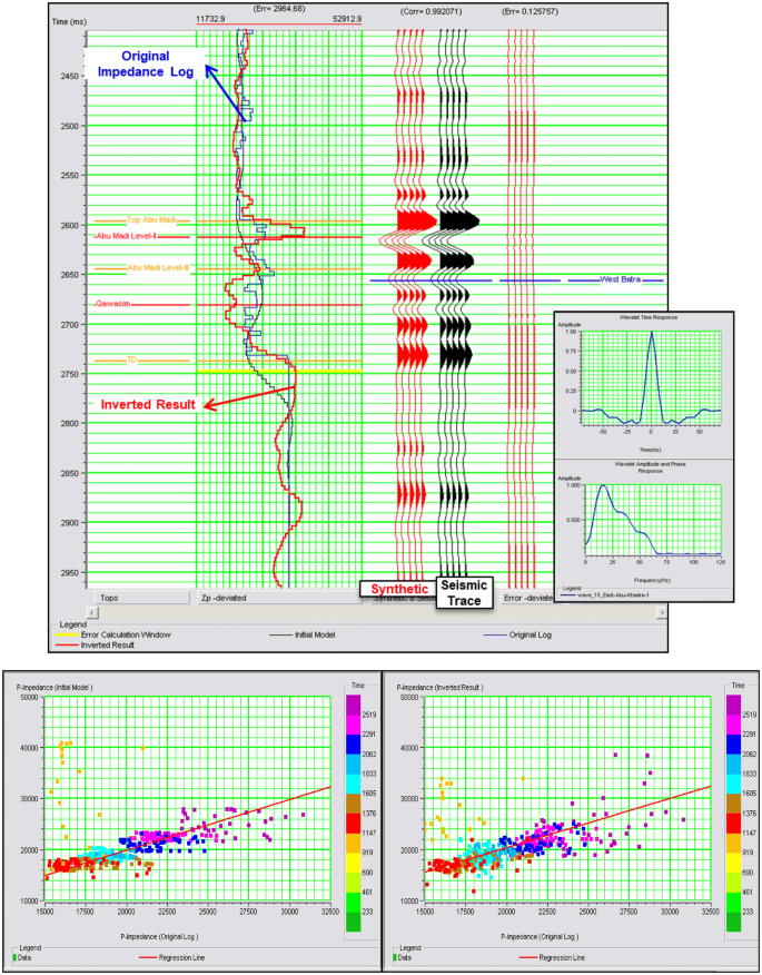

  

  Pre-stack analysis for QC the initial inversion results

Precise estimate of wavelet for calculating synthetic for the seismic inversion success and likewise relies on a perfect tie between the well to seismic. As the wavelet shape has effects in the inversion results, subsequent assessment of the reservoir management is dependent to the selected wavelet (Barclay et al. 2008).

Results and discussion

The petrophysical analysis shows that the gas well discovery has penetrated Qawasim sandstone facies with a good reservoir quality have average porosity 32%, water saturation 18% and total gas reading up to 163, 500 ppm with components up to N40, which indicates that this zone may contain a wet gas. While the dry well has penetrated Qawasim sands has zero net pay with average porosity 23% and water saturation 95% (Fig. 16).

Fig. 16

The petrophysical analysis and results of the two drilled wells

The modeling and analysis of the CDP gathers on Near, Mid and Far-angles of the two drilled wells have been concluded that, there is a great variation between the results of the two prospects, even though the seismic characters of the amplitude anomalies in the stacked sections are similar to a great extent and have the same structure and stratigraphic sequence. The authors have found that, the gas well (Fig. 17, left) has a full offset coverage. In other words, the Near-offset traces are completely recorded, as well as the Far-offset. Therefore, in this case, there is a true amplitude anomaly, which can be verified by observed the amplitude gradual increase with offset on the Near, Mid and Far angles seismic stack, which may reveal a hydrocarbon fluid effect, which can be also verified by the extraction of different attributes such as fluid factor and (intercept × gradient) AVO attributes (Figs. 11 and 12).

Fig. 17

CDP gathers for both the gas-bearing and dry wells, showing the missing of Near-offset traces at the dry well

On the other hand, the CDP gather of the dry well (Fig. 18), the complete absence of the amplitude response in the Near-offset can be observed and it is starting from the Mid-offset, causing the pseudo bright amplitude anomaly that confirmed with the failure of drilling well results. In other cases, it can be found that, the Near-offset does not exist at all (Fig. 19), this is may be due to some surface obstacles during the field data acquisition, as an example in the urban areas or agricultural areas, especially when the acquisition commenced in a highly cultivated, mountains and populated areas, hence, it cannot be considered at all. Therefore, the step of revising the CDP gathers in the Near and Far-offsets should be adding to the prospect evaluation main criteria such as direct hydrocarbon indicator (DHI)’s, seismic polarity, AVO response with offset, structure element and low-frequency shadow (Fig. 20). So, these mentioned criteria can be used to differentiate between reservoirs and non-reservoirs, in addition to the pre-stack CDP gathers verification.

Fig. 18

CDP gather on the exact dry well location, shows the missing of near-traces, due to some urban surface obstacles during acquiring the seismic data in the field

Fig. 19

Near-offset coverage map, showing the complete missing of the near-offset traces due to surface obstacle where the area is a highly cultivated terrain

Fig. 20

Near-offset seismic section illustrate hole or complete missing of the Near-offset traces at the dry well location due to some urban surface obstacles at the prospect drilled location

In our research, the pre-stack inversion applied (Fig. 21), we analyze the fully processed CDP gathers to generate volumes of Zp, Zs and density cubes (Fig. 22). After estimating the Rp and Rs from the AVO analysis, as discussed, we can proceed to invert the Rp, which will give the p-wave acoustic impedance, Zp = $\rho$Vp, and inverting Rs give the S-wave impedance, Zs = $\rho$Vs.

Fig. 21

Zp versus Zs and Zp versus density croosplots for analyzing inversion results

Fig. 22

Final output for the inversion (acoustic imped. P-wave, S-wave and density cubes)

Concerning the results of the inversion, by determining the density, the fizz water problem can be solved. Figure 23 elucidates the P-wave inversion final result, whereas the P-wave low impedance denotes the gas sand. The results of the inversion around a certain prospect can be tolerated with the closest wells. Also, the anisotropy has a potential impact on the results led to variation on the AVO response and acoustic impedance model, due to facies changes of the different lithology, due to the deltaic environments deposits characteristics.

Fig. 23

Arbitrary line between the proposed locations of two gas wells from the inverted cube

Moreover, the outcomes of the pre-stack inversion will assist in the reservoir quality evaluation. Accordingly, there are three cases (Fig. 24), the first of which is the upper one for a non-economic gas well, where the slight decrease in the acoustic impedance can be seen, owing to the weak dissimilarity between the gas sand and the overlying shale, which may indicate a bad reservoir quality in this well. The second is the middle case for a gas well (used as a blind well), where a sharp contrast between the shale and the gas sand can be seen, which is confirmed by the sharp decrease in acoustic impedance in the pay zone. The third is the lower case for a prospect which resembles, to a great extent, the middle case. Therefore, from this display, the reservoir quality in gas wells can be evaluated which will also help in the prospect evaluation.

Fig. 24

Vertical sections from the inverted seismic data cube

Limitations and uncertainties in AVO applications

We use the AVO as a tool for recognizing and validating the presence of hydrocarbons, reducing the risk of drilling a dry hole or passing over a profitable discovery. However, we find there are several pitfalls during the application, due to the limitation of the technique, caused by misleading data, complex lithology combinations and thickness variations.

Non-commercial gas saturation

Traditional 2-term AVO will not be able to discriminate between a seismic anomaly caused by a few percent gases and an anomaly caused by commercial amounts of hydrocarbon. This is a universal problem and many wells have been drilled on AVO driven prospects that indicated hydrocarbons, but proved to be residual amounts of gas. These were scientifically correct, but commercial failures. 3-terms AVO calculating density, to estimate gas saturation, is based on the linear behavior of density with gas saturation. However, uncertainty factors, such as the poor signal-to-noise ratio and the effect of anisotropy at mid to far offsets make the 3-terms AVO difficult.

Data quality problem

Seismic artifacts can cause a false AVO anomaly. Unfavorable acquisition conditions can lead to data problems, which can be seen in El Mansoura area, such as weak/no signal at the Near-offsets, due to the limited data fold, noisy Far-offset, or weak/no reflection for some deeper formations. Some problems are processing related, such as the Far-offset high amplitude and low frequency by NMO, residual move-out, and offset dependent amplitude scaling and poor application of data muting.

Rock property

During the AVO application in the study area, find the chance of success is generally higher in the clastic sand/shale environment, rather than carbonate the environment. Modeling found the high amplitude is more likely, a lithology indictor than the fluid indictor in limestone environment.

Conclusions

The weak seismic coverage has been affected on the seismic amplitude anomaly reliability, structure geometry and the AVO response with offset. So, the analysis of the CDP gathers on different angles, verification of the AVO response can help in evaluate the potentiality of the prospects and determine the response of the seismic amplitude variation with the offset. The AVO analysis and pre-stack modeling allow the interpreter to: (1) Understanding the seismic signature, due to the wave propagation. (2) Defining the reservoir rock physical properties. (3) Integrating seismic, well logs, lab testing and VSP information, to verify the reservoir conditions. Pre-stack modeling is effective to:

(a) Examining the seismic response, due to lithology’s physical properties, such as porosity, fluid content and reservoir and pay thickness. (c) Substituting the pore fluid and modeling the seismic response. (d) Varying the reservoir properties and model the seismic response. (e) Exploring the uniqueness of possible seismic interpretation. (f) Evaluating the exploration potential and recognizing the exploration risk. (g) Processing the synthetic gather, to extract attributes to understand, which may be useful.

References

Abdel Halim M (2001) Future hydrocarbon potential in the Nile Delta offshore and onshore. In: Zaghloul ZM, El-Gamal M (eds) Deltas modern and ancient. Proceedings of 1st international symposium on the deltas, March 13–19, 1999, Cairo, Egypt, pp 159–174
Barclay F, Bruun A, Alfaro JC, Cooke A, Cooke D (2008) Seismic Inversion: Reading Between the Lines. Schlumberger Oilfield Review
Cardamone M, Ciurlo B, Noli V (2007) AVO and fluid Inversion, ENI
Castagna JP, Swan HW (1998) Principles of AVO cross-plotting. Lead Edge 16:337–342
Chopra S, Sharma RK (2016) Preconditioning of seismic data prior to impedance inversion. https://explorer.aapg.org/story?articleid=24631
Dahroug AM, Sharafeldin SM, Mabrouk WM, Noaman MH (2018) Contribution of integrating seismic coherency and AVO attributes in delineating sand bars reservoirs, Offshore Nile Delta, Egypt, a case study. Egypt J Pet 27:595–603
EGPC (Egyptian General Petroleum Corporation) (1994) Nile Delta and North Sinai: field discoveries and hydrocarbon potentials (a comprehensive overview). Egyptian General Petroleum Corporation, Cairo, p 387
Hampson D, Russell B (2006) The old and the new in seismic inversion. Tulsa Convention Centre, Calgary, December 18, 2006
Hampson D, Russell B, Bankhead B (2005) Simultaneous inversion of pre-stack seismic data. SEG Technical Program Expanded Abstracts. Hampson-Russell Software Services Ltd, and Brad Bankhead, VeritasDGC, p 2668
Kamel H, Eita T, Sarhan M (1998) Nile Delta hydrocarbon potentiality, Egypt. In: Proceedings of 14th EGPC exploration and production conference, Cairo, pp 485–503
Latimer RB, Davison R, van Riel P (2000) An interpreter’s guide to understanding and working with seismic-derived acoustic impedance data. Lead Edge 19:242–256
Nanda NC (2016) Seismic data interpretation and evaluation for hydrocarbon exploration and production. A practitioner’s guide. Springer, Cutack
Nastaran M, Mokhtari M (2016) Application of post stack and pre stack seismic inversion for prediction of hydrocarbon reservoir in a Persian Gulf gas field. Int J Environ Chem Ecol Geol Geophys Eng 10(8):853–862
Nini C, Checchi F, El Blasy A, Talaat A (2010) Depositional evolution of the Plio-Pleistocene succession as a key for unraveling the exploration potential of the post-Messinian play in the Central Nile Delta. MOC
Russell B (2014) Seismic reservoir characterization and pre-stack inversion in resource shale plays. Calgary, Canada, Posted October 27, 2014
Rutherford SR, Williams RH (1989) Amplitude-versus-offset variations in gas sands. Geophysics 54:680–688
Verm R, Hilterman F (1994) Lithology color-coded seismic sections: the calibration of AVO cross-plotting to rock properties. Lead Edge 14:847–853
Yilmaz O (2001) Seismic data processing. Society of Exploration Geophysicists, Tulsa
Author information
Authors and Affiliations
Corresponding author
Additional information
Publisher's Note
Springer Nature remains neutral with regard to jurisdictional claims in published maps and institutional affiliations.
Rights and permissions
Open Access This article is distributed under the terms of the Creative Commons Attribution 4.0 International License (http://creativecommons.org/licenses/by/4.0/), which permits unrestricted use, distribution, and reproduction in any medium, provided you give appropriate credit to the original author(s) and the source, provide a link to the Creative Commons license, and indicate if changes were made.
About this article
Cite this article
Hussein, M., El-Ata, A.A. & El-Behiry, M. AVO analysis aids in differentiation between false and true amplitude responses: a case study of El Mansoura field, onshore Nile Delta, Egypt. J Petrol Explor Prod Technol 10, 969–989 (2020). https://doi.org/10.1007/s13202-019-00806-2
Received:
Accepted:
Published:
Issue Date:
DOI: https://doi.org/10.1007/s13202-019-00806-2