
Abstract
Amplitude variation with offset (AVO) analysis is an important tool for identifying natural gas-bearing reservoirs. The changes in seismic amplitudes based on the variation of density and velocity of the rock matrix are captured through the AVO analysis. The current work was performed in the Ghotaru region of the Jaisalmer Sub-basin area, where limited and discrete hydrocarbon discoveries were observed from the Lower Goru Formation during the earlier various exploration campaigns. The discrete nature of the reservoir lithofacies developed challenging scenarios for the successful exploratory campaign. The campaign encountered more difficulties because of limited advanced datasets, which affected the study to capture the extension of hydrocarbon-bearing reservoir lithofacies and its characterization towards a successful exploration campaign. This study shows the way to overcome these challenges using an existing conventional dataset. The study shows the possibility of AVO analysis using a post-stack seismic dataset. A unique conversion method from post-stack to pre-stack seismic is introduced in this study based on the uses of the integrated velocity model. An integrated, robust velocity model was developed with consideration of anisotropy factors. Introducing a machine learning-based algorithm in the petrophysical study, including the conventional approach, provides a robust validation of this work. Intercept (A) and gradient (B) are the basic outcome of AVO analysis. The well-based study and AVO analysis based on intercept (A) and gradient (B) complement each other for finding hydrocarbon-bearing reservoir rock. Cross-plots and AVO analysis show the reservoir's lithofacies extension and fluids. The study reveals the potential of natural gas retained in the Lower Goru Formation, which is composed of patchy sandstone. Two AVO classes (Class I and Class III) of gas-bearing sandstone have been identified in this study. This study presents a unique method for identifying natural gas reservoirs with limited old conventional data.
Introduction
The present work is performed in the Jaisalmer Sub-basin, which is a part of the Rajasthan Basin. Rajasthan Basin is considered a prolific hydrocarbon-bearing province in India. A significant portion of the Jaisalmer Sub-basin is a part of the Rajasthan Shelf. This basin widens to the Mari region in this area and has been converted to a part of the Indus Basin. Study shows that the hydrocarbon migration from the Indus Basin to the Jaisalmer Sub-basin occurred during the Cretaceous age (Boruah 2010). However, the significant discovery of hydrocarbon is limited in this sub-basin because of the complex reservoir structure and frequent changes in the reservoir lithofacies. The present work has been accomplished in the Ghotaru region, where hydrocarbon-bearing lithofacies are present with limited discoveries. The geological character of the formation displays the probability of getting natural gas in this area. However, due to a limited geoscientific dataset, a limitation for conducting an advanced level of integrated geoscientific study has been observed in this area. Identifying natural gas over seismic images requires AVO analysis. AVO analysis tracks seismic reflection amplitude changes. AVO analysis is capable of identifying the reservoir lithofacies and characterizing the fluid property (Chiburis et al. 1993) by capturing the variations in the physical properties (Cardamone et al. 2007) of the rock that influence the seismic amplitudes across the boundary (Dahroug et al. 2017) in most of the geological settings. To conduct AVO analysis, pre-stack seismic data are required where a variation of seismic amplitude is captured with offset. This amplitude variation produces the anomaly between reservoir and non-reservoir lithofacies due to the presence of fluid. The analysis works more prominently in the gas reservoir. Compressional and shear sonic data are also necessary for AVO analysis to understand reservoir behaviour. In this study, the AVO analysis was performed without the support of pre-stack seismic and shear sonic (S-sonic) data. The full workflow was designed based on the conversion process from post-stack seismic and conventional well log data. A unique approach was adopted to convert the conventional geoscientific data into required data for AVO analysis. The study was limited to the Lower Goru Formation of the early cretaceous age, and it is composed of shale and clay with occasional sandstone. To support the results from AVO analysis, a comprehensive petrophysical analysis was performed to understand the reservoir properties over conventional data. The machine learning algorithm is also used to detect patterns of reservoir lithology and rock properties in the Lower Goru Formation. The cluster analysis technique is used for this purpose to get effective results in this geological setting. Machine learning (ML)-based petrophysical analysis (McDonald 2021) produced less uncertain results with effective support for the AVO analysis. In this study area, significant heterogeneities are observed in the reservoir section in the Lower Goru Formation. The heterogeneities have been taken care of through the incorporation of anisotropy parameters in the study. Development of the integrated velocity model was crucial in our study, where anisotropy factors were also taken care of. In view of anisotropic condition of earth’s geometry (Rosid et al. 2018), we used the anisotropic aspect of P-sonic velocity by considering Thomsen anisotropy parameters epsilon (ε) and delta (δ) in the current study. The analysis shows the interpretation of post-stack seismic data AVO inversion in the Ghotaru region of the Jaisalmer Sub-basin area to depict gas reservoirs within the field using AVO inversion techniques. The assumption behind the AVO analysis has its origin in the Zoeppritz equations through angle dependent variation of reflection coefficient (Muskat and Meres 1940).
The study of model-based AVO shows a comprehensive comparison between seismic-based common offset shot gather and models which are generated during AVO analysis (Russell and Hampson 1991). The developed integrated expression (Aki and Richard’s 2002) during AVO analysis represents significant anomalies in reference to the mudrock line in the seismic data (Smith and Gidlow 1987; Castagna et al. 1985) which shows hydrocarbon in the reservoir. The integrated expression was simplified to capture the feasible variation of primary wave reflection coefficient (Fatti et al. 1994) where pre-stack seismic data provide significant information in the form of petrophysical and rock physical properties (Aki and Richards’ 1980) during AVO analysis. Different forms of attribute analysis based on AVO outcomes such as intercept (A) and gradient (B) produce distinct result to identify the hydrocarbon (Rutherford and Williams 1989) including challenging reservoir condition (Castagna and Smith 1994).
We conducted the current study in the Ghotaru area of the Jaisalmer Sub-basin with suitable analogue data support from the Bandha region of the same sub-basin. Figure 1 demonstrates the study area.

The study wells and analogue well locations are positioned in the geographic map of the Jaisalmer Sub-basin, a part of Rajasthan Basin
The integrated outcome from AVO inversion and machine learning-based petrophysical analysis provides worthy information in the Ghotaru region of the Jaisalmer Sub-basin. Current research shows possibilities for multiple discoveries of natural gas from the Lower Goru Formation in the study area.
Geology of the study area
Rajasthan Basin is situated in the northwest part of India, encompassing the west and northwest of Aravallis up to the Indo-Pakistan border. The basin is a pericratonic basin that establishes a portion of the Indus Geosyncline with a 5000 m span of average sediment thickness. Geologically, the Rajasthan Basin has expanded from a period of Cambrian to a recent one. The basin has been split into three sub-basins distinguished from each other by ridges and faults. These sub-basins are Jaisalmer, Bikaner-Nagaur, and Barmer-Sanchor Sub-basin. The present study concentrates on the Jaisalmer Sub-basin. The northwest Pokhran-Nachna High separated Jaisalmer from the Bikaner-Nagaur Basin and the Barmer Basin in the south by the Banner-Birmama-Nagarparkar High/Fatehgarh Fault. The Jaisalmer Sub-basin is noticeable as a northwest–southeast trended territorial fault-bound region from Jaisalmer to Mari (Awasthi 2002). It is estimated that the Jaisalmer Basin is a Late Palaeozoic-Mesozoic basin with a mild slope of 30 to 50 dip and composed of Permian-age rocks that unconformably lie over the Proterozoic basement. Jaisalmer Sub-basin is divided into three depressions, i.e., Shahgarh Depression, Kishangarh Shelf, and Miajlar Shelf. The current study area comes under the Shahgarh Depression and Kishangarh Shelf region.
Progressions of hydrocarbon spanning in age from Jurassic to Eocene include a good number of organic elements, and total organic carbon content (TOC) of 1–2% is present in the Goru, Pariwar, Baisakhi, and Bedesir Formations (Singh and Mandal 2015). A small amount of algal amorphous organic element exists. In general, kerogen is of Type III and is gas-prone (Biswas 2012). Various organic-rich shale formations are recognized as source rocks, such as Lower Goru, Pariwar, Baisakhi-Bedesir shales, and Karampur/Badhaura shales (Pandey et al. 2019; Wandrey et al. 2004). The Pariwar sandstones, Lower Goru sandstones, and Sanu or Khuiala sandstones of the Late Paleocene and Early Eocene are identified as the reservoir quality of the Jaisalmer Basin (Dwivedi 2016). We accomplished this study by focusing on the sediments of the Lower Cretaceous age, which spread from Lower Goru to the Pariwar Formation. The current study mainly concentrates on the Lower Goru Formation, which has a thickness of 211 m, and it is dominated by shale lithology. The study was performed with a limited data set of the Ghotaru region, and for anisotropic computational needs, analogue well data of the nearby identical sedimentary basinal structure of the Bandha region are used.
Available data
In the study area, dataset was limited in the form of conventional approach which was more than 30-year-old acquired data. In view of limited data availability, we used several empirical relations in this study to get required support from the existing dataset (Faust 1953; Han et al. 1986; Prasad 2002; Lee 2010 and Gardner et al. 1974) (Table 1).
Methodology
The AVO inversion process was adopted as a quantitative interpretation technique, which is considered the most feasible study for identifying gas-bearing reservoirs (Dvorkin et al. 2014; Bredesen et al. 2021). Quantitative interpretation covers various potential studies where advanced datasets are required; in this analysis, AVO inverted results can reach the objective. A dataset of 3D seismic post-stack line and ten exploration wells marked W-1 to W-10 were chosen for the AVO analysis. The post-stack seismic data quality is good based on the amplitude–frequency distribution representation. The seismic data bandwidth varies between 12 and 66 Hz. There is no skewness present in the amplitude spectrum, showing a uniform distribution. The inversion process begins with the well-to-seismic tie process, which correlates well with seismic data. In this process, optimized filters are used in the time and frequency domain to condition the wavelets, which produce a robust result. The analysis displays the fluctuation in acoustic impedance characteristics of the rock. A conversion process using an anisotropic integrated velocity model was applied to convert the full-stack migrated zero offset seismic volume into pre-stack seismic data such as angle stack and offset gathers. Before executing seismic amplitude analysis, it is crucial to know the petrophysical properties of the study area. Conventional, log-based manual prediction of facies distribution involves numerous uncertainties, especially when the working dataset is large. Hence, an unsupervised machine learning based on a clustering technique using well log data was implemented to characterize the reservoir rock type precisely. After completion of the petrophysical assessment of the Lower Goru Formation, AVO forward modelling and attribute extraction was carried out using CGG/GeoSoftware Hampson-Russell software. The other significant parts of this research work were carried out in different software and languages, such as M/s Schlumberger Petrel, CGG/ GeoSoftware Jason, MATLAB, and Python. Table 2 demonstrates the rock property variation from ten exploratory wells in the Lower Goru Formation.
Conditioning of well data and rock physics modelling
Lower Goru Formation does have the potential for hydrocarbon exploration; however, due to limited advanced study in the challenging reservoir, the broad scope for successful exploration is not visible in the study area. Primary data for advanced study are unavailable in many wells, such as P-sonic and density logs. This study adopted the rock physics modelling approach for estimating these log data. Rock physics models develop reservoir static models using well log and seismic data in an integrated approach. Knowledge of well log data is crucial for wavelet extraction, and seismic data gives bandlimited frequency. The information obtained from quantitative well-to-seismic tie supports rock physics modelling. The entire work was carried out according to the following workflow (Fig. 2.).

A precise workflow of well log data editing and conditioning
The rock physics model was initiated by conditioning the available well log data, which were used as input data to develop the empirical rock physics model. Necessary support was considered from the Hashin–Shtrikman bound model during the development of the rock physics model; the support of the Hashin–Shtrikman bound model was considered based on the structural characteristics of the reservoir rock in the Lower Goru Formation. This bounding model presents the upper and lower bounds of the effective moduli of the rock by knowing each constituent’s volume fraction and elastic moduli (Mavko et al. 2009).
As the depth of investigation of sonic (P and S) and density logs are small, these logging tools are affected by problems linked to borehole rugosity, washouts, and mud filtrate invasion. Editing of well data begins with recognizing noticeable issues like washouts, mud filtrate invasion effects, cycle skipping, and anomalous values on elastic logs over cross-plots, log plots, and histogram analysis. By using a rolling median filter, the log data was despiked (Tiwary et al. 2009). After the proper conditioning of well data, a better well and seismic data correlation has been achieved.
A significant limitation of the data of the Lower Goru Formation is the missing \({V}_{P}\),\({V}_{S}\), and density log measurements in some wells. The missing parameters \({V}_{P}\),\({V}_{S}\), and density are crucial as they represent the rock’s geological properties (composition and consolidation) and control the seismic response with increased offset. This study used a power regression empirical equation between P wave velocity and density with the proper consideration of study interval and identical lithology. For predicting density values, modified Gardner’s relation (Gardner et al. 1974) (Eq. 1) was applied, while the estimation of P wave velocities was done based on Eq. 2 (Faust 1953).
where \(a\) and \(b\) are constants and \(\rho\), \({V}_{P}\) are the density and P wave velocity.
where \({V}_{P}\) is the P wave velocity in feet/second, \(a\) is a constant, \(R\) is the resistivity value in ohm feet and \(Z\) is the depth in feet.
In (Sayers et al. 2011) Rock physics study in the Gulf of Mexico, the \({V}_{P}\)-\({V}_{S}\) relation of (Castagna et al. 1985) was applied for the local substitution of missing \({V}_{S}\) logs and gave descent \({V}_{S}\) values. This study also used this \({V}_{P}\)-\({V}_{S}\) relation using the \({V}_{P}\) logs of the Lower Goru Formation and presented reasonable \({V}_{S}\) output.
In the above relation, the unit of velocity is in kilometres/second.
Well correlation and calibration with post-stack seismic
Well data correlation is one of the crucial analyses for this study, where the identified reservoir section in the Lower Goru Formation was correlated between study wells. The significance of the structural correlation shows an extensive upliftment of the shallower formations in the surrounding areas, affecting the hydrocarbon maturation and migration. Figure 3 shows the well correlation between Ghotaru and Bandha regions, where tectonic changes are well observed in the Lower Goru Formation. Four wells, i.e., W-2, W-4, W-6, and W-8, have been considered in the Ghotaru area, whereas the name of the analogue well was considered from the Bandha region. The analysis of the analogue well provides support to get information on the deposition of gas-bearing reservoir lithofacies in the Ghotaru region.

Well correlation between W-2, W-4, W-6, and W-8 of the Ghotaru area and Analogue well of the Bandha area
The well-to-seismic tie method is the initial step in calibrating facies and lithology obtained at the well location to seismic volume. Suitable wavelet extraction and development of the time-to-depth relationship was the prime objective of the well-to-seismic tie. P-sonic data were used in all wells for time-to-depth calibration. The well-to-seismic tie process provides support in the quantitative interpretation based on amplitude, phase, and frequency fluctuation (Datta Gupta et al. 2021). Figure 4 presents the time response of the extracted statistical wavelet used in this work and its corresponding amplitude-phase-frequency spectrum on the bottom. The process of the well-to-seismic tie was carried out in all nine study wells (Figs. 5, 6, 7, 8, 9).

Statistical wavelet time response and corresponding amplitude-phase-frequency spectrum on the bottom

Development of synthetic seismogram with a favourable correlation between synthetic and seismic data of W-1 and W-2

Development of synthetic seismogram with a favourable correlation between synthetic and seismic data of W-3 and W-4

Development of synthetic seismogram with a favourable correlation between synthetic and seismic data of W-5 and W-6

Development of synthetic seismogram with a favourable correlation between synthetic and seismic data of W-7 and W-8

Development of synthetic seismogram with a favourable correlation between synthetic and seismic data of W-9
Wavelet is considered a significant parameter in this process as frequency and phase obtained from wavelet greatly influence the correlation coefficient result from tying well data to seismic. Wavelet, in general, acts as a convolution operator between seismic data and surface reflectivity. There are three ways in which a wavelet can be extracted,
-
i.
A process in which the linear phase is considered a zero phase.
-
ii.
At least square method in which assumption about phase is not considered.
-
iii.
At least square method in which phase is considered on the basis of correlation present in between reflectivity of log and surface seismic.
The algorithms used in the wavelet extraction process are categorized into deterministic, statistical, multi-well, and analytical. In the correlation process between the reflection coefficient of a well and seismic traces, the use of an appropriate filter to know the wavelet is necessary. Phase and frequency values are obtained from the inverse filter. At first, the time lag of the wavelet is removed on the basis of bulk shift, and for additional fine-tuning, the wavelet is placed at zero time. The extracted wavelet is used to develop a synthetic seismogram correlated with real seismic traces to achieve a good correlation coefficient.
Analysis of Reservoir Rock property
Petrophysical analysis interprets data to estimate lithology, porosity, facies, and fluid saturation. A petrophysical assessment was performed in the Lower Goru Formation of the study well W-3. Unsupervised machine learning algorithms are studied for recognizing lithology and facies distribution in Ghotaru (Bormann et al. 2020). Analysis of petrophysical parameters such as porosity and saturation is essential to capture the distribution of lithofacies since these parameters vary depending on the types of facies. Well log data is used to analyse key petrophysical properties such as porosity, permeability, saturations, and rock volumes of the reservoir.
Unsupervised cluster analysis for lithofacies discrimination
Two unsupervised clustering methods, i.e., K-means clustering and Gaussian mixture modelling (GMM), are adopted in this study, and the outcome of these cluster models was compared with an established lithofacies curve. Cluster analysis involves grouping data points of similar characteristics into one cluster and those that are different put into another cluster. Four logs, i.e., gamma ray (GR), bulk density (RHOB), neutron porosity (NPHI), and acoustic compressional slowness (DT), are used in the establishment of the cluster model.
-
(i)
K-means clustering
\(J\) = Objective function, \(k\) = number of clusters, \(N\) = number of observations, \({x}_{i}^{(j)}\)= Observation, and \({C}_{j}\)= centroid for cluster j.
In this method, the initialization of the centroid at \(k\) random points is done in the data space, and the data points surrounding the centroid are assigned to the appropriate cluster depending on the distance to the centroid. Then, according to the central point of the cluster, the centroid is adjusted, and the data points encompassing it are reassigned. This process continues until centroids remain in the same position, data points persist in the same cluster, or maximum iterations have been attained. This K-means cluster analysis is a hard-clustering process where a circle is applied to the data to perform clustering.
-
(ii)
Gaussian mixture modelling (GMM)
In the Gaussian mixture modelling process, data points are clustered based on data variance and hence adopt a soft clustering approach. The Gaussian mixture models are probabilistic models where ellipsoidal-shaped clusters are formed depending on probability density estimations using the expectation–maximization (EM) technique. The EM method is fundamentally a statistical algorithm used to determine the optimum model parameters when the data has missing values or is incomplete. The EM algorithm has primarily two steps:
-
a.
E-step This step uses the available data to determine (guess) the missing variable values.
-
b.
M-step Based on values obtained from the E-step, the parameters are updated using the entire data.
GMMs consider a particular number of Gaussian distributions; each distribution represents a single cluster. The Gaussian probability distribution or normal distribution is represented as (Bishop 2006)
\(\mu\) = D-dimensional mean vector, \(\sum\) = D X D covariance matrix which defines the Gaussian shape and \(\left|\Sigma\right|\)= determinant of \(\Sigma\)
A Gaussian mixture model is defined as the linear combination of the fundamental Gaussian probability distribution and is described as
\(K\) = Number of components in the mixture model, \({\pi }_{k}\) = mixing coefficient that provides a density estimate of individual Gaussian component. The Gaussian density, i.e., \(N\left(X|{\mu }_{k},{\Sigma}_{k}\right)\), is known as a component of the mixture model. Each component k is defined by a Gaussian distribution with a mean of \({\mu }_{k}\), covariance of \({\Sigma}_{k}\) and mixing coefficient of \({\pi }_{k}\).
For the efficient working of K-means and GMM models, an initial number of clusters are provided to the models. This study considers silhouette analysis combined with elbow plot methods to precisely identify the optimum number of clusters. The silhouette plot measures the compactness of each point in one cluster compared to the neighbouring cluster, thus, estimating the number of clusters visually. The plot has a range of [− 1,1]. A silhouette score of + 1 signifies the best, i.e., the data points are very compact within the cluster and very distant from other clusters. The worst score is − 1; a near 0 score indicates an overlapping cluster. The elbow method employs K-means clustering on the dataset for a varying range of K. K signifies the number of cluster values. Let the K values vary from 1 to 30. In this method, inertia (i.e., the sum of the squared distances to the nearest cluster centre) against the number of clusters is plotted and looked up for the elbow point where there is a shift in the rate of decrease. The elbow point indicates the optimum number of clusters. An equal number of clusters is used in both K-means and GMM models to simplify the comparison. After establishing both K-means and GMM models, the data are plotted to understand how well these models predict lithology with respect to labelled lithology.
Estimation of reservoir properties
The geophysical logs (gamma, resistivity, neutron, density, and sonic) are used in the quantitative assessment of shale volume (\({V}_{\mathrm{\rm sh}}\)), effective porosity (\({\phi }_{\mathrm{eff}}\)), and water saturation (\({s}_{\mathrm{w}}\)).
-
(i)
Calculation of volume of shale
Shale volume estimation is significant as it assists in evaluating formation porosity, fluid content, and reservoir rock quality. This study adopts gamma ray log methods to obtain shale volume.
where \(\mathrm{IGR}\) = gamma ray index, \(\mathrm{IGR}\)=\({V}_{\mathrm{\rm sh}}\) in the linear model, \(\mathrm{GRlog}\)= gamma ray reading of the formation, \(\mathrm{GRmin}\) = minimum gamma ray reading, and \(\mathrm{GRmax}\) = maximum gamma ray reading.
Precise estimation of shale volume is a necessary as it affects other petrophysical properties such as effective porosity and water saturation (Chikiban et al. 2022).
-
(ii)
Calculation of porosity
Estimation of porosity was highly significant during this study towards the characterization of the reservoir. We estimated effective porosity based on the initial estimation of total porosity from well log data.
The combination of neutron and density logs helps estimate total porosity (\({\phi }_{\mathrm{T}})\) within the reservoir interval.
where \({\phi }_{\mathrm{N}}\)= neutron porosity, \({\phi }_{\mathrm{D}}\) = density porosity
where \({\rho }_{\rm ma}\) = rock matrix density, \({\rho }_{b}\) = bulk density comprising both rock and fluid density, and \({\rho }_{f}\)= fluid density.
We estimated the effective porosity (\({\phi }_{\rm eff})\) based on the modification of total porosity according to the estimated shale volume.
where \({\phi }_{T}\) = total porosity, \({\phi }_{\rm sh}\) = porosity reading in a shale zone, and \({V}_{\rm sh}\) = shale volume
-
(iii)
Calculation of water saturation (\({{\varvec{s}}}_{{\varvec{w}}})\)
The water saturation is characterized as the ratio of water volume to pore volume. The resistivity and porosity logs (neutron, density, and sonic) helped in the calculation of \({s}_{w}\). Initially both Archie’s (1942) and Simandoux’s (1963) empirical relations were used for estimating water saturation in this study. However, based on character of the reservoir rock of this sub-basin Simandoux (1963) produced considerable outcomes.
\({R}_{T}\) is the resistivity of the rock in ohm meter, \({R}_{W}\) is the formation water resistivity in ohm meter, \({s}_{w}\) is the water saturation, \(a\) is the formation factor constant, \(m\) is the cementing factor, \(n\) is the saturation component, \(\phi\) is the porosity, \({R}_{\rm sh}\) is the resistivity of shale, and \({V}_{\rm sh}\) is the shale volume.
To get a comprehensive knowledge about the behaviour of reservoir rock. The bulk volume of water (BVW) is estimated by using the multiplication of the calculated water saturation (\({s}_{w})\) and its corresponding porosity (\(\phi\)).
-
(iv)
Calculation of hydrocarbon saturation (\({{\varvec{s}}}_{{\varvec{h}}})\)
The percentage of hydrocarbon present in the pore volume of a formation is known as hydrocarbon saturation. This study estimates this by subtracting the water saturation value from 100%, i.e.
-
v.
Net to GROSS (NTG)
The ratio between the sand-bearing hydrocarbon thickness and the total sand formation thickness is known as the net to gross (NTG). A proper estimation of NTG ratio is essential for this kind of heterogeneous reservoir to capture the actual pay zone. In view of challenging geological condition of the reservoir, the NTG is estimated based on variation of maximum estimated porosity of the study zone and porosity of specific depth.
Development of integrated velocity model and estimation of Thomsen parameters
Shale is the dominant rock type of the Lower Goru Formation, and as shale is intrinsically anisotropic, it consistently affects seismic data, including seismic velocities. The anisotropy values estimated from seismic and vertical seismic profile (VSP) have poor resolution and are principally based on the P wave. Well data are usually used for good resolution. This study uses P and S wave data of vertical wells to estimate Thomsen’s anisotropic parameters with improved resolution. Shale is typically considered transversely isotropic (Vernik and Nur 1992). In normal cases, a vertically transverse isotropic (VTI) model is chosen for a simple depositional structure with a vertical axis of symmetry. This indicates that the velocity calculated along the symmetry axis will be constant, but different values are obtained when calculated vertically.
In the case of a VTI model, the elastic stiffness tensor analysis consists of five independent elements, i.e.
where \({m}_{11}\)=\({m}_{22}\), \({m}_{33}\), \({m}_{12}={m}_{21}\),
Borehole velocity propagates in three directions (X, Y, and Z), and on the basis of these directional fluctuations, anisotropy parameters are evaluated. Three axial planes (X1, X2, and X3) are chosen for measuring velocity distribution. This study considers vertical wells, so X3 is the borehole axis, and along X1–X2, plane formation is isotropic (Fig. 10).

A simplified diagram for qualitative representation of anisotropy parameters estimation in accordance with the plane of symmetry (modified after Pradhan et. al 2019)
To estimate the Thomsen anisotropy parameters (ε, γ, and δ), both SX and SY components of shear sonic are necessary. Based on the identical geological property, an analogue well (W-AN) of the Bandha region is selected with 184-268 m depth taken for study. Equation (3) estimates the SX component, and the SY component is evaluated through a normalization approach between the study and analogue well. This approach considers a product of variation of SX and SY components of the analogue well and compressional velocity variation of study and analogue well.
In a transversely isotropic medium, the Thomsen anisotropy parameters are represented over the P wave velocity propagation in the vertical direction and S wave velocity in the rotating condition along the X3 axis, and the three parameters are illustrated as (Thomsen 1986; Mavko et al. 2009)
The wave propagating in the \({X}_{i}\) axis and polarized in the \({X}_{j}\) axis is known as \({V}_{ij}\). The relation between \({V}_{ij}\) and stiffness coefficient \({m}_{ij}\) in the transversely isotropic condition is (Ostadhassan et al. 2012; Pradhan et al. 2019).
To completely describe a vertically transverse isotropic (VTI) medium, \({m}_{33}\), \({m}_{55}\), \({m}_{66}\), \({m}_{11}\) and \({m}_{13}\) are essential. \({m}_{33}\), \({m}_{55}\) and \({m}_{66}\) are computed from Eq. (17), and \({m}_{11}\) and \({m}_{13}\) are evaluated by considering the ANNIE model hypothesis.
The ANNIE model (Shoenberg et al. 1996) assumes
In a VTI medium, \({m}_{44}\) and \({m}_{55}\) are considered variable parameters to depict each term. After replacing all the five constants (\({m}_{11}\), \({m}_{13}\), \({m}_{33}\), \({m}_{55}\), and\({m}_{66}\)) in Eqs. (14,15,16), we acquired the values of ε, γ, and δ. Two main aspects for the evaluation of Thomsen parameters are \({V}_{12}\) and \({V}_{13}\). The SY factor is considered \({V}_{12}\), and the SX factor is taken as \({V}_{13}\) for all wells.
Velocity polarizes in different directions as it is a vector quantity (Fig. 11). The velocities in the symmetry directions are the compressional (\({V}_{p0}\)) and shear wave velocities (\({V}_{s0}\)). This study assumed that the measured sonic velocities are phase velocities (Ellefsen et al. 1989). Thomsen’s equations are also applied in the case of weak anisotropy. The S wave polarized in the perpendicular direction to the symmetry is known as \({V}_{SH}\), and in the parallel direction to the symmetry is known as \({V}_{SV}\). The transverse direction of \({V}_{SV}\) and \({V}_{s0}\) is identical; hence, they are the same in the transverse isotropy system. \({V}_{PH}\) is known as horizontal P wave polarization.

A schematic model for illustrating velocity polarizations in different directions for a transverse isotropic media
In an anisotropic medium, the equation of motion relating the elastic coefficient and velocity of the tensor matrix is
\({m}_{ijkl}\) = elastic coefficients, \({n}_{j}\) and \({n}_{l}\) = elements of normal wave front, \(\rho\) = density, \(v\) = phase velocity,\(\delta\) = Kronecker delta function, \(and\, P\) = unit displacement vector
This wave equation is resolved to an eigenvalue equation on the basis of Fourier (plane wave) comprising three eigenvectors (polarization vectors) and three respective eigenvalues (velocities) in each propagation direction. In a weak polar anisotropic medium, these three velocities are approximated as (Thomsen 1986)
Post-stack to pre-stack seismic data conversion
Before converting post-stack (zero offsets) to pre-stack seismic data, a comparative plot between P-sonic velocity and polar anisotropic P-sonic velocity was carried out to signify the effect of anisotropy on velocity. Compressional velocity obtained from Eq. 20 was taken as anisotropy incorporated P-sonic velocity. In this study, we considered two cases based on angle variation and its effectiveness: (i) near-angle stack (θ = 10º) and (ii) far-angle stack (θ = 30º). The plot presents certain wells with noticeable velocity deflections due to anisotropy that adversely affects the outcome if it is not correctly captured. Hence, correct estimation of anisotropy parameters of shales and incorporation of these parameters into the velocity model substantially enhances seismic reservoir characterization.
In the velocity model, velocity varies laterally, i.e., velocity variations along with the offset, so the offset was estimated from this velocity model, and the super gather or common offset gather was constructed. The super gather assembles traces within a box by the offset and common midpoint (CMP) ranges. This process also generates average common depth points (CDP) to reinforce the signal-to-noise (S/N) ratio. During this process, the super gather manages the AVO amplitude and preserves the offset dimension. Normal moveout (NMO) is applied to the gather to align primary events. AVO analysis begins with transforming offset domain CMP gathers to angle domain. Seismic data are measured on offset (x), and for transforming from fixed offset to fixed angle(θ) domain, a relationship is required between these two parameters. There are two approaches to this: (i) the straight ray method and (ii) the ray parameter method.
-
i.
The straight ray method
This method adopts the following equation
\({v}_{rms}\) = layer root mean square (RMS) velocity
\({t}_{0}\) = two-way reflection time.
As mentioned above, the formula considers that the reflection rays propagate as a straight path between the surface and the reflecting point. The angle is resolved from the above relation when the layer RMS velocity, offset, and two-way travel time are known.
-
ii.
The ray parameter method
This method is authentic for all velocities, offsets, and times where a two-term NMO equation exists and does not require the condition of a linear velocity gradient. Since we have NMO corrected gather, this approach is appropriate for estimating the angle of incidence. Considering Snell’s law, the ray connecting to the reflecting point is assumed to be bending, i.e., refracting, and \({v}_{i}/\mathrm{sin}(\theta )\) acts as a constant along the ray. A ratio of the RMS velocity to the sample time and the local interval velocity helps estimate the angle of incidence (Yilmaz 2001). The equation is
\({v}_{i}\) is the interval velocity, \({v}_{r}\) is the RMS velocity, and \({t}_{0}\) is the two-way reflection time.
A limit of 300 is utilized in AVO inversion as higher angles create complications in eliminating normal moveout. This study uses the ray parameter method to convert offset domain CMP gather to angle domain. Once the data are in the pre-stack angle domain, AVO inversion is carried out.
Amplitude variations with offset: modelling and analysis
This study focuses on how the reservoir properties fluctuations affect the seismic response on the basis of forward AVO modelling. In forward AVO modelling (to produce a synthetic seismogram), exact Zoeppritz equation was used to estimate the reflection coefficient as a function of incident angle, i.e., R(ɵ). Zero-phase Ricker wavelet was convolved with these reflection coefficients to develop the synthetic CDP gathers at various fluid saturations. The assessment of AVO is accomplished by fitting the time sample amplitude of a gather to an expression that connects reflectivity at a given angle (offset) to compressional and shear wave reflectivities. The complicated Zoeppritz equations illustrate that along a particular interface, the plane elastic wave reflection coefficient depends on the reflection angle (Aki and Richards 2002).
The above equation is further approximated by (Wiggins et al. 1983; Russell 1988)
The above equations display the connection present in amplitude and \({\mathrm{sin}}^{2}\left(\theta \right)\). Intercept and gradient are the most typical AVO attributes used in the hydrocarbon industry. Compressional velocity and density are the only parameters affecting intercept (A), as shown in Eq. 30. The AVO gradient (B) relies upon compressional, shear velocities and density, according to Eq. 31. The term gradient primarily affects AVO inversion. At the small angle of incidence, below 30°, the curvature factor (C) has minimal effects on the amplitude to drop this term. Hence, we obtain a reflection coefficient in a common midpoint gathered by applying only the first two portions of Aki and Richards’s relation.
Shuey (1985) further analysed the Zoeppritz equation and dissolved the reflectivity part to normal incidence; corrections primarily rely upon Poisson’s ratio and density fluctuations over an interface.
The first term in the above equation depicts the zero-degree angle of incidence amplitude. The next portion illustrates a mid-angle amplitude modification. The last portion defines the wide-angle amplitude. We concentrate only on mid-angles; hence, we can drop the third term.
The AVO analysis begins by extracting typical AVO attributes, intercept, and gradient. These factors estimate secondary attributes, A × B and A + B, scaled Poisson’s ratio variation, and the generation of cross-plots to recognize and discriminate reservoir fluids and lithology. The AVO cross-plotting technique is significant in determining the AVO classification (Castagna and Swan 1997) and recognizing oil and gas (Ross and Kinmann 1995). In specific geological cases, intercept and gradient in shale and water–sand layers display a particular background tendency. AVO anomalies that show divergence from this background tendency indicate hydrocarbons or lithology factors.
AVO for isotropic and anisotropic case
A comparative study between isotropic and anisotropic conditions has been carried out to illustrate the importance of anisotropy parameters in AVO analysis. The subsurface anisotropy affects the seismic amplitude; hence, velocity dependence on an angle will lead to variations in amplitude to reflectivity and from reflectivity to offset.
AVO for isotropic case
The three-term Shuey equation, which approximates the reflection coefficient from the Zoeppritz equation, is used to compute the reflection coefficient in terms of incidence angle. Thus, the equation for the isotropic case is
\({R}_{P}\) is the P wave reflection coefficient, \(\mathrm{and} \,\theta\) is the incidence angle
\({V}_{P}\), \({V}_{S}\), and \(\rho\) are average P wave, S wave velocity, and density along an interface, respectively.
\(\Delta {V}_{P}\), \(\Delta {V}_{S},\) and \(\Delta \rho\) are P wave, S wave velocity, and density change along an interface, respectively.
AVO for anisotropic case
For an anisotropic case, the same three-term Shuey equation is used.
\({R}_{P}\left({\theta }_{a}\right)\) is the P wave reflection coefficient, and \({\theta }_{a}\) is the wavefront angle
The incidence angle is considered as the wavefront angle and
\({V}_{Pa}\) and \({V}_{SVa}\) are average P wave polar anisotropy velocity and average SV wave polar anisotropy velocity obtained from Eqs. 20 and 21, respectively.
\(\Delta {V}_{\mathrm{Pa}}\), \(\Delta {V}_{\mathrm{SV}a},\) and \(\Delta \rho\) are change along an interface in each P wave polar anisotropy velocity, SV wave polar anisotropy velocity, and density, respectively.
\(\Delta \varepsilon\) and \(\Delta \delta\) are anisotropy parameters change across an interface.
A pictorial depiction of the AVO inversion analysis adopted in the current study is shown in Fig. 12.

A precise systematic workflow for performing AVO inversion process
Results
Interpretation of well-to-seismic tie
The elementary segment of this study comes from the process of well to seismic ties. In the Lower Goru Formation, the zone of interest was marked as the study zone top, and the bottom and statistical wavelets were extracted within this zone. These recognized zones’ depth ranges differed for all ten study wells. All the extracted wavelets were in the zero phases. In the process of the well-to-seismic tie, we achieved a maximum cross-correlation coefficient of 72.8% in well W-6 and a minimum of 43.4% in well W-9. The cross-correlation coefficient fluctuates from 40 to 70%, a reasonable value for this study. Figures 5, 6, 7, 8,9, and Table 3 illustrate the characteristics of all extracted wavelets from all nine study wells. In the Ghotaru region, most of the drilled wells were very old; hence, a limited data set is available. A low cross-correlation coefficient is found in well W-9 due to the unavailability of the dataset, and all logs are obtained from transform relationships (Gardner et al.1974) (Faust 1953).
Petrophysical assessment based on machine learning (ML) algorithm
Lithofacies distribution is a crucial element in reservoir modelling which provides sedimentological characteristics of reservoir rock and assists in the estimation of intrinsic properties of a reservoir, such as porosity, water saturation, etc. The conventional approach to facies distribution comprises the classification of facies according to the depositional environment obtained from the primary well data available at a particular depth interval. This approach incorporates numerous uncertainties and is tedious as primary data are also missing in some wells of the study area and is estimated empirically using transformed relationships (Gardner et al. 1974; Faust 1953). The shale cut-off volume is another approach to facies classification, but this method also involves many ambiguities. An advanced technique is highly required to predict facies distribution with minimum uncertainty. Hence, this study considers machine learning algorithms to identify facies distribution. There are two techniques in machine learning, i.e., supervised learning and unsupervised learning algorithms. A supervised algorithm requires labelled datasets to classify data and predict the outcome, whereas an unsupervised algorithm does not need it. Typical conventional well log responses of the well W-3 provide a comprehensive idea about the reservoir in the study area. To represent most considerable and focused results in the study area under ML and petrophysical sections, we have mentioned well W-3 only in this manuscript. The study well W-3 does not have labelled data, so an unsupervised clustering technique is used to identify the hidden patterns within the data.
Clustering results
-
I.
Data visualisation
Five lithofacies, i.e., siltstone, shale, sandstone, clay, and silty-shale, were identified in the Lower Goru Formation of W-3. Neutron–density cross-plots or scatter plots have been carried out for each respective lithology to understand the data distribution over each lithofacies of W-3 (Fig. 13).
Fig. 13 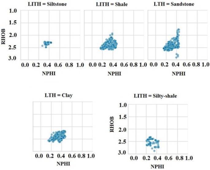
Data distribution for each lithologies identified within the study well W-3
-
ii.
Recognition of optimum number of clusters
Figure 14a shows the silhouette plot for 1314 samples in 10 clusters (labelled from 0 to 9) with an average silhouette score of 0.395. The silhouette plot for cluster 9 has a maximum thickness, and cluster 7 has a minimum thickness. Due to this wide variation in the thickness of the silhouette plot of each cluster, consideration of 10 clusters is suboptimal. Figure 14b represents the link plot between the number of clusters and the silhouette score. In this figure, when the number of clusters 4, 5, and 6 is considered, a change in slope occurs at the number of clusters 5. Hence, based on silhouette analysis, the number of clusters can be taken as 5.
Fig. 14 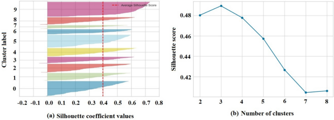
a. Silhouette analysis for K-means clustering on 1314 samples with number of clusters 10 b. Silhouette plot between number of clusters and silhouette score
Fig. 15 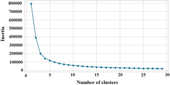
Elbow plot for the selection of the optimum number of clusters
Figure 15 shows the elbow plot where there is a change in slope ahead of the 5-number cluster. Hence, both the silhouette and elbow plot methods suggest 5 as the optimal number of clusters.
-
iii.
Comparison between K-means and GMM model output
Figure 16 illustrates the log plot of W-3 in the first four columns, the original lithofacies (LITH_SI), and the estimated K-means and GMM cluster outputs in the last three subplots. Five distinct facies or groups are shown in the plot and are largely tied up with variations in log data. In this figure, the topmost section of the Lower Goru Formation, the decrease in gamma from 1070 to 1080 m, is tied perfectly in the lithology subplot with three layers of variations, i.e., blue, light orange, and yellow. In the K-means and GMM, this portion is also marked in the same cluster, with K-means showing two-layer variation (yellow and maroon), whereas GMM shows no variation (marked by yellow). In the middle portion of the Lower Goru Formation from 1125 to 1200 m, the original log lithofacies exhibits three-layer variations (marked by orange, light orange, and yellow). The same segment in the K-means and GMM model illustrates four-layer variations (marked by orange, light orange, yellow, and maroon). The last 25 m of this section from 1175 to 1200 m K-means model exhibits more thin-layer variations than GMM. The lower segment of the Lower Goru Formation, i.e., the part where gamma decreases from around 1215 m to 1255 m, is tied with orange and light orange groups in the lithology subplot. In the K-means and GMM models, this portion is also marked in the same cluster with very few variations. K-means illustrates two thin-layer variations, and GMM shows a single thin layer. Thus, one can conclude that K-means gives much more thin-layer variations than GMM in the Lower Goru Formation of W-3.
Fig. 16 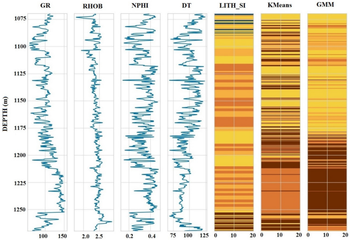
Well log plot illustrating original lithology, K-means and GMM models output in the Lower Goru Formation of W-3
-
iv.
Cluster output in scatterplots or cross-plots and pair plots
A neutron–density scatterplot or cross-plot is carried out to display the output of the cluster analysis (Fig. 17). Though the clusters are overlapped in each method, the earlier mentioned portion, i.e., the 1215 to 1255 m depth zone of the log plot, can be recognized in the K-means in the lower right of the scatterplot marked in orange with high density, high neutron porosity values. By comparing K-means and GMM cluster outputs with the supplied lithology, it is observed that K-means model results match closely with the lithology provided.
Fig. 17 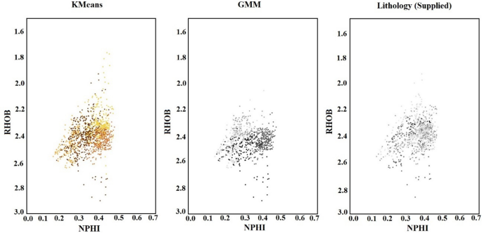
Cross-plot comparison of unsupervised learning (K-means and GMM) outputs with the supplied lithology
As four input curves (GR, RHOB, NPHI, and DT) are used to establish K-means and GMM models, pair plots have been developed to show the cluster variations with respective data used (Fig. 18). The distribution of data split per cluster is also plotted in the diagonal direction.
Fig. 18 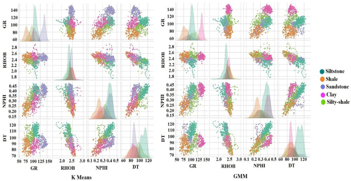
Comparison between K-means model and GMM model pair plot showing different cluster variations for each input curve


The pair plot presents the variation of data clustered in other logging curves in an improved manner. It can be observed that K-means gives better results in illustrating the clusters, specifically in the DT versus GR plot.
Petrophysical evaluation of reservoir
Figure 19 captures the variations of the reservoir properties in the conventional well log data including computed petrophysical log data in the well W-3 within the study zone of the Lower Goru Formation. Besides a machine learning-based approach, this study uses the gamma ray (GR), neutron porosity (NPHI), density (Rhob), resistivity (LLD), and compressional sonic (P-sonic) logs to identify the lithological unit across the Lower Goru Formation. In this study we have observed significant responses in GR, NPHI, and Rhob log data. In the neutron–density combination plot, low neutron and density log values shows sandstone formation as higher values of neutron and density depicted shale. In Fig. 19, the GR value shows a dominant increment in the range of 1215 to 1255 m depth which shows the maximum value of 150 API and along with large neutron–density values indicating the shale section. An opposite trend has been observed in the GR values at depth range of 1085 to 1105 m, 1110 to 1120 m, and 1155 to 1170 m, it suggests the presence of sandstone in the Lower Goru Formation. A graphical representation (Fig. 20) on the variations of lithology in the well W-3 captures the nature of the reservoir where separation of specific hydrocarbon-bearing lithology is a challenging task as the distribution pattern is mixed and overlapped to each other. Histogram analysis shows that the presence of shale in the study zone of the Lower Goru Formation is maximum, whereas the presence of siltstone is minimum (Fig. 20). Table 4 shows the summery of estimated crucial petrophysical parameters of the well W-3 within the study zone which captures the potentiality of the specific zone as a reservoir in the Lower Goru Formation.

Petrophysical interpretation of the Lower Goru Formation in W-3

Nature of distribution of lithology within the study zone of the Lower Goru Formation in the well W-3; histogram analysis shows the quantified presence of different lithology within the study zone
Anisotropy effect on velocity and AVO
The plots in Figs. 21, 22 justify the importance of anisotropy parameters in an integrated velocity model to obtain a robust outcome. Both plots display the effect of polar anisotropy on P-sonic velocity. It compares the normal and polar anisotropy P wave velocity at the near-angle stack, θ = 10º, and far-angle stack, θ = 30º for all ten study wells. Minimal velocity fluctuations are observed at the near-angle stack. Hence, polar anisotropy velocity for the far-angle stack is calculated. In wells W-1, W-3, W-4, W-5, W-7, and W-10, minor velocity fluctuations are detected (Fig. 21), but in wells W-2, W-6, W-8, and W-9 in (Fig. 22), noticeable deflections are observed between normal and polar anisotropic P wave velocity. In (Fig. 22 b) for W-2, velocity deviation is prominent at (1100–1200 m) in the far-angle stack, and another variation occurs at 1250 m. The other wells of Fig. 22, i.e., W-6, W-8, and W-9, show velocity deviations at specific points. This is noticed at (1150 m, 1250 m, 1270 m, and 1300 m) for W-6 (Fig. 22 f), (1270–1300 m, 1400–1430 m) for W-8 (Fig. 22 d), and (1250 m, 1320 m) for W-9 (Fig. 22 h). Lastly, one can conclude that the effect of anisotropy at the far-angle stack is maximum for wells shown in Fig. 22 and minimum for wells represented in Fig. 21. The least velocity difference at the far angle is observed in Fig. 21 due to the missing P-sonic logs in these wells and is estimated from the transformed relationship (Faust 1953).

A comparative study between standard P wave and anisotropy incorporated P wave velocity at near angle 10º and far angle 30º for wells with minimal velocity fluctuations at far angle

A comparative study between standard P wave and anisotropy incorporated P wave velocity at near angle 10º and far angle 30º for wells with noticeable velocity fluctuations at far angle
A comparative plot of incidence angle versus reflection coefficient (obtained from Eq. 37,41) for the isotropic and anisotropic conditions in all ten study wells has been illustrated in (Fig. 23).

A comparative study between isotropic and anisotropic AVO plot for all ten study wells, where the reflection coefficient is unitless and angle of incidence (ɵ) is in degree
At zero angle of incidence, positive reflection coefficient with values in the range of 0.01–0.1 has been observed in all ten study wells for both isotropic and anisotropic cases. The reflection coefficient’s absolute value, i.e., the amplitude, has reduced with the increase in the angle of incidence for both cases. The plot shows that for the anisotropy case, the intercept values of the \({R}_{0}\) amplitude reduce with the increase in offset or incidence angle until it becomes negative (i.e., for wells W-1, W-2, W-3, W-4, W-5, W-8, W-9, W-10) and remain positive for some wells (i.e., W-6 and W-7). Likewise, for the isotropic condition, the reflection coefficient decreases with increasing angle of incidence but persists in positive value. The two data points coincide at a small angle of incidence; however, these points begin to deviate with the increase in the angle of incidence around 100–150. This comparative analysis signifies the influence of Thomsen’s anisotropy parameters (ε and δ) on AVO based on the fluctuation of phase velocity as a function of the incidence angle, as shown in Eqs. 20 and 21. The phase velocity is a crucial parameter in influencing the reflectivity of the transverse isotropic medium. Hence, incorporating anisotropy parameters into the velocity model is essential, eventually capturing the reservoir robustly.
Interpretation of established pre-stack angle stack seismic data
The conditioned seismic interval velocity is integrated with well anisotropic velocity to develop the pre-stack angle stack seismic data (Fig. 24). This unified anisotropic velocity model tied to all wells covered in the study area was implemented in converting post-stack seismic data to pre-stack seismic data.

Integrated velocity model using seismic and well log velocity, the model has been centred in the target horizon of 500-1100 ms; the model was used for the generation of pre-stack seismic data
Figure 25 displays the simultaneous representation of data in the offset and angle domains, respectively. Moreover, this represents a comparative demonstration between full-stack (Fig. 25 a) and converted angle stack (Fig. 25 b) seismic data; the converted angle stack seismic is considered a near-angle stack. The conversion process to the angle domain has been carried out based on the ray parameter changes method within the time window of 500 to 1100 ms; this time window was identified based on the presence of the reservoir

a. Zero offset CDP stack seismic data b. angle stack near gather; in both cases the inserted curve data is the P wave
Figures 26 and 27 show amplitude variation in the full-stack and converted angle stack seismic data through the study wells (well 1 to well 10) within the time window of the reservoir zone

Full scale zero offset seismic wells representing all ten wells within the target horizon 500 ms-1100 ms

Super gather (common offset stack) produced from the 3D seismic data
AVO attributes identification
The AVO attributes are significant in recognizing lithology and pore fluid variations using AVO anomalies. In this section, we have analysed the outcome of AVO attributes and illustrated how these attributes effectively identify hydrocarbon fluids, i.e., oil and gas, from background geology.
Intercept
A linear regression study was performed to estimate the intercept (A), which is the best linear fit to the AVO data with zero offsets, i.e., the cut-off on the amplitude axis (R0) (Fig. 28). This attribute recognizes the zero offset amplitude directly related to the reflection coefficient computed in (Eq. 29). In (Fig. 29), the light whitish-to-red fluctuations mark the + ve intercept, i.e., high attribute values. The whitish-to-blue variations depict − ve intercept, i.e., low attribute values.

Linear fit to AVO data with sin2 (incidence angle) along X-axis and amplitude along Y-axis

Extracted intercept within the working horizon of 500 ms to 1100 ms where red colour marks + ve intercept and blue colour shows − ve intercept
Gradient
The gradient is known as the slope of the optimum fit to AVO, i.e., the slope of the regression line in a cross-plot of amplitude versus \({sin}^{2}\left(\theta \right)\) and expresses the relative change in amplitude with angle and offsets (Fig. 28). Figure 30 displays the extracted gradient where red signifies high and blue signifies low attribute values.

Extracted gradient within the working horizon of 500 ms to 1100 ms where red colour marks + ve gradient and blue colour shows − ve gradient
Intercept product gradient (A X B)
It is a common practice in AVO analysis to estimate an A X B attribute, i.e., intercept X gradient, which is simply the multiplication of two primary attributes. Figure 31 shows this attribute, where the peak denotes a rise in amplitude with offset, and the trough expresses a diminish in AVO. The outcome of this product is consistent + ve (red) in AVO Class III, as the gradient and the intercept are of identical character (+ ve or − ve). Nevertheless, in Class Ι, these attributes are of different characters (+ ve and − ve); hence, multiplication is forever − ve (blue) (Fig. 31). In this study, the A X B attribute indicates Class Ι anomaly, representing the high impedance sands, the intercept marginally reduces, and the − ve gradient substantially rises. Thus, the colour delineates the multiplication of intercept and gradient, highlighting AVO anomaly. By comparing this AVO anomaly with resistivity and VP logs, one can observe the similarity in the gas-saturated sand and AVO pattern.

Product of the intercept and gradient within the working horizon of 500 ms to 1100 ms; here the product is − ve
Gradient X Sign (intercept)
The product of the gradient and sign of the intercept attribute preserves the gradient value, but the polarity fluctuates with the combined polarities of the gradient and intercept (Fig. 32).

Product of the gradient and sign (intercept) with in the working horizon of 500 ms to 1100 ms where red marks + ve gradient x sign (intercept) and blue shows − ve gradient x sign (intercept)
Intercept X Sign (gradient)
The intercept and sign of the gradient multiplication attribute retain the intercept value. However, the polarity varies with the combined polarities of the intercept and gradient (Fig. 33).

Product of the intercept and sign (gradient) within the working horizon of 500 ms to 1100 ms where red marks + ve intercept x sign (gradient) and blue shows − ve intercept x sign (gradient)
Poisson’s ratio change
The sixth attribute is an excellent confirmation of the existence of gas-saturated sediments. Scaled Poisson’s ratio displays fluid fluctuations present in the reservoir. This attribute is the most favourable method to delineate the AVO anomaly using colour data, where Poisson’s ratio varies from 500-1100 ms (Fig. 34). Foster et al. (1993, 2010) illustrated that sand can retain higher or lower acoustic impedance than the encircling shale; however, gas sand attains a lower Poisson ratio than shale or brine sands. One can obtain the compatibility between gas sand and the low Poisson’s ratio by comparing Poisson’s ratio with resistivity and VP. Thus, low Poisson’s ratios are an excellent confirmation for gas favoured by wells W-1, W-2, W-3, and W-5, and a small portion of well W-6 and W-9, marked as orange (Fig. 34). No gas zone discovered in well W-4, W-7, W-8, and W-10.

Scaled Poisson’s ratio displaying fluctuation in accordance with the fluid present in the reservoir; here, small values represent gas supported by well W-1, W-2, W-3, W-5, W-6, and W-9 with orange colour
AVO cross-plots
AVO cross-plot is one of the most straightforward approaches in analysing the different variable relationships. The plot displays the linear relationship between the AVO intercept and AVO gradient. The cross-plot accomplishes entire time samples at trace positions inside a definite window. Any divergence from this system is an indication of hydrocarbon. When the fluid density diminishes, the intercept–gradient pair proceeds distantly from the background line tendency. Hence, very clear, distinct gas sands will be observed. The deviation from the background line tendency (AVO anomalies) is because of the rock's stiffness, fluid content, and porosity. Figure 35 illustrates the cross-plot between the AVO intercept and AVO gradient with proper identification of distinct classes for each AVO anomaly zone. The analysis is carried out within a time window of 426–1118 ms.

Cross-plot for AVO intercept and AVO gradient
Three different cases, i.e., pessimistic (P-10), base (P-50), and optimistic (P-90) trend lines, were plotted in the AVO cross-plot (Fig. 35).
The linear relation for the pessimistic case is given by
where y = AVO gradient and x = AVO intercept. The correlation coefficient is 0.885689.
The linear equation for the base case is given by
where y = AVO gradient and x = AVO intercept. In this case, a convincing correlation coefficient of 0.932305 (i.e., > 90%) has been attained.
The linear equation for the optimistic case is given by
where y = AVO gradient and x = AVO intercept. The correlation coefficient is 0.978920.
Fluctuations of the gradient values have been captured through the uncertainty analysis based on P-10, P-50, and P-90 evaluation. Subsequently, after analysing all the cases, the gradient values vary between a maximum of 380.592 to a minimum of − 371.615 (Fig. 36).

Capture of the uncertainty of the measured gradient values from the AVO cross-plot based on P-10, P-50, and P-90 analysis
AVO study and interpretation are performed by delineating the background line tendency and outlining points far from the background line. Distinct colours emphasize this because its AVO class specifies the beginning and end of the gas zones in the cross-plot.
Conclusions
The Ghotaru area is geologically active and has the potential for oil and gas exploration. Discrete lithofacies and complex reservoir architecture make hydrocarbon exploration difficult in this area. The exploration work faced more difficulty because of the presence of a limited dataset. In the current study, the possibilities of hydrocarbon exploration in this area rejuvenates based on empirical relation-based conversion. In this study, possible geological uncertainties of the reservoir were taken care of through anisotropy analysis. Machine learning-based petrophysical analysis provided a robust integrated outcome to reach the aim of this study.
-
I.
In the current research work, post-stack seismic is converted to pre-stack, with comprehensive weightages in the computed anisotropy factors in the integrated velocity model for AVO analysis. We identified that this unique process is the most authenticated and proven approach for AVO analysis in this geological set-up where the dataset is limited.
-
II.
K-means cluster algorithm over GMM of ML-based analysis provides the most accepted lithofacies distribution patterns to capture hydrocarbon-bearing facies.
-
III.
Analysis shows the presence of patchy discrete sandstone in the reservoir, which is considered as reservoir lithofacies in the Lower Goru Formation.
-
IV.
AVO inversion and AVO-based attribute analysis show the presence of both Class I and Class III gas-bearing sandstone in the reservoir of the Lower Goru Formation.
Abbreviations
- A :
-
Intercept
- \(a\) :
-
Constant
- B :
-
Gradient
- \(b\) :
-
Constant
- C :
-
Curvature factor
- \({C}_{j}\) :
-
Centroid for cluster j
- GRlog :
-
Gamma ray reading of the formation, API
- GRmin :
-
Minimum gamma ray reading, API
- GRmax :
-
Maximum gamma ray reading, API
- IGR :
-
Gamma ray index
- \(J\) :
-
Objective function
- \(k\) :
-
Number of clusters
- \(K\) :
-
Number of components in the mixture model
- \(m\) :
-
Cementing factor
- \({m}_{ij}\) :
-
Stiffness coefficient in the \({X}_{i}\) direction and polarized in the \({X}_{j}\) direction
- \({m}_{11}\) :
-
Stiffness constant in a plane in which shear wave is propagating and polarized in the X1 direction
- \({m}_{13}\) :
-
ANNIE model estimated stiffness constant
- \({m}_{33}\) :
-
Stiffness constant in the perpendicular axis
- \({m}_{55}\) :
-
Stiffness constant in a vertical plane comprising compressional wave in the X3 axis and shear wave in the X1 axis
- \({m}_{66}\) :
-
Stiffness constant in a horizontal plane comprising shear wave in the X1, X2 axes
- \({m}_{ijkl}\) :
-
Elastic coefficients
- \(N\) :
-
Number of observations
- \(n\) :
-
Saturation component
- \({n}_{j}\) , \({n}_{l}\) :
-
Elements of normal wave front
- \({P}_{k}\) :
-
Unit displacement vector
- \(R\) :
-
Resistivity, Ω ft
- \({R}_{P}\) :
-
P wave reflection coefficient
- \({R}_{\rm sh}\) :
-
Resistivity of shale, Ω m
- \({R}_{T}\) :
-
Rock resistivity, Ω m
- \({R}_{W}\) :
-
Formation water resistivity, Ω m
- \({R}_{S}\) :
-
S wave reflection coefficient
- \({s}_{h}\) :
-
Hydrocarbon saturation
- \({s}_{w}\) :
-
Water saturation
- \({t}_{0}\) :
-
Two-way reflection time, s
- \({V}_{ij}\) :
-
Wave velocity propagating in the \({X}_{i}\) direction and polarized in the \({X}_{j}\) direction, m/s
- \({V}_{P}\) :
-
P wave velocity, m/s
- \({V}_{Pa}\) :
-
Average P wave polar anisotropy velocity, m/s
- V PH :
-
Horizontal P wave polarization, m/s
- \({V}_{p0}\) :
-
P wave velocity parallel to the axis of symmetry, m/s
- \(\Delta {V}_{P}\) :
-
P wave velocity change along an interface, m/s
- \(\Delta {V}_{\rm Pa}\) :
-
Average P wave polar anisotropy velocity change along an interface, m/s
- \({V}_{S}\) :
-
S wave velocity, m/s
- V SH :
-
S wave polarized in the perpendicular direction to the symmetry, m/s
- \({V}_{\rm sh}\) :
-
Shale volume
- V SV :
-
S wave polarized in the parallel direction to the symmetry, m/s
- \({V}_{s0}\) :
-
S wave velocity parallel to the axis of symmetry, m/s
- \({V}_{\rm SVa}\) :
-
Average SV wave polar anisotropy velocity, m/s
- \(\Delta {V}_{S}\) :
-
S wave velocity change along an interface, m/s
- \(\Delta {V}_{\rm SVa}\) :
-
Average SV wave polar anisotropy velocity change along an interface, m/s
- \({V}_{11}\) :
-
Shear wave velocity travelling and polarized in the X1 direction, m/s
- \({V}_{12}\) :
-
Shear wave velocity along the X1 direction, differentiated in the X2 direction, m/s
- \({V}_{13}\) :
-
SX component obtained from compressional wave velocity, m/s
- \({V}_{33}\) :
-
Compressional wave velocity propagating and polarized along the X3 direction, m/s
- \(x\) :
-
Offset distance, m
- \({x}_{i}^{(j)}\) :
-
Observation
- \(Z\) :
-
Depth, ft
- \(\gamma\) :
-
Thomsen anisotropy parameter gamma
- \(\delta\) :
-
Thomsen anisotropy parameter delta
- \({\delta }_{ik}\) :
-
Kronecker delta function
- \({\Delta \delta }\) :
-
Anisotropy parameter delta change across an interface
- \(\varepsilon\) :
-
Thomsen anisotropy parameter epsilon
- \({\Delta \varepsilon }\) :
-
Anisotropy parameter epsilon change across an interface
- \(\theta\) :
-
Incidence angle, degree
- \({\theta }_{a}\) :
-
Wavefront angle, degree
- \(\mu\) :
-
D-dimensional mean vector
- \({\pi }_{k}\) :
-
Mixing coefficient which provides a density estimate of individual Gaussian component
- \(\rho\) :
-
Density, g/cm3
- \({\rho }_{b}\) :
-
Bulk density comprising both rock and fluid density, g/cm3
- \({\rho }_{f}\) :
-
Fluid density, g/cm3
- \({\rho }_{\rm ma}\) :
-
Rock matrix density, g/cm3
- \({\Delta \rho }\) :
-
Density changes along an interface, g/cm3
- \(\Sigma\) :
-
D X D covariance matrix defining the Gaussian shape
- \(\left|\Sigma\right|\) :
-
Determinant of \(\Sigma\)
- \(\sigma\) :
-
Poisson’s ratio
- \({\Delta \sigma }\) :
-
Change in Poisson’s ratio
- \(v\) :
-
Phase velocity, m/s
- \({v}_{i}\) :
-
Interval velocity, m/s
- \({v}_{r}\) :
-
RMS velocity, m/s
- \({v}_{\rm rms}\) :
-
Layer RMS velocity, m/s
- \(\phi\) :
-
Porosity
- \({\phi }_{D}\) :
-
Density porosity
- \({\phi }_{\rm eff}\) :
-
Effective porosity
- \({\phi }_{N}\) :
-
Neutron porosity
- \({\phi }_{\rm sh}\) :
-
Porosity reading in a shale zone
- \({\phi }_{T}\) :
-
Total porosity
- API:
-
American petroleum institute
- AVO:
-
Amplitude variation with offset
- CDP:
-
Common depth point
- CMP:
-
Common mid-point
- DT:
-
Acoustic compressional slowness
- EM:
-
Expectation-Maximization
- GMM:
-
Gaussian mixture modelling
- GR:
-
Gamma ray
- ML:
-
Machine learning
- NMO:
-
Normal move out
- NPHI:
-
Neutron porosity
- RHOB:
-
Bulk density
- RMS:
-
Root mean square
- TOC:
-
Total organic carbon content
- VSP:
-
Vertical seismic profile
- VTI:
-
Vertical transverse isotropic
- W-AN:
-
Analogue well
References
Aki K, Richards PG (1980) Quantitative seismology: theory and methods. W H Freeman Co, San Francisco
Aki K, Richards PG (2002) Quantitative seismology: theory and methods, 2nd edn. University Science Books, Sausalito
Archie GE (1942) The electrical resistivity log as an aid in determining some reservoir characteristics. Trans AIME 146(01):54–62. https://doi.org/10.2118/942054-G
Awasthi A M (2002) Geophysical exploration in Jaisalmer Basin: a case history. Geohorizons: 1–6
Bishop CM (2006) Pattern recognition and machine learning. Springer, Berlin
Biswas SK (2012) Status of petroleum exploration in India. Proc Indian Natn Sci Acad 78:475–494
Bormann P, Aursand P, Dilib F, Manral S, Dischington P (2020) Force 2020 Well well log and lithofacies dataset for machine learning competition. https://doi.org/10.5281/zenodo.4351156
Boruah N (2010) Rock physics template (RPT) analysis of well logs for lithology and fluid classification. In: 8th biennial international conference and exposition on petroleum geophysics, Society of Petroleum Geophysicist, Hyderabad, pp. 1–8
Bredesen K, Rasmussen R, Mathiesen A, Nielsen LH (2021) Seismic amplitude analysis and rock physics modelling of a geothermal sandstone reservoir in the southern part of the Danish Basin. Geothermics. https://doi.org/10.1016/j.geothermics.2020.101974
Cardamone M, Ciurlo B, Noli V (2007) AVO and fluid inversion. ENI
Castagna JP, Smith SW (1994) Comparison of AVO indicators: a modelling study. Geophysics 59(12):1849–1855. https://doi.org/10.1190/1.1443572
Castagna JP, Swan HW (1997) Principles of AVO cross plotting. Lead Edge 16(4):337–342. https://doi.org/10.1190/1.1437626
Castagna JP, Batzle ML, Eastwood RL (1985) Relationships between compressional-wave and shear-wave velocities in clastic silicate rocks. Geophysics 50(4):571–581. https://doi.org/10.1190/1.1441933
Chiburis E, Franck C, Leaney S, McHugo S, Skidmore C (1993) Hydrocarbon detection with AVO. Oilfield Rev 6:42–50
Chikiban B, Kamel M H, Mabrouk W M, Metwally A (2022) Petrophysical characterization and formation evaluation of sandstone reservoir: a case study from Shahd field, Western Desert, Egypt. Contribut Geophys Geodesy 52(3): 443–466. https://doi.org/10.31577/congeo.2022.52.3.5
Dahroug AM, Sharafeldin SM, Mabrouk WM, Noaman MH (2017) Contribution of integrating seismic coherency and AVO attributes in delineating sand bars reservoirs, Offshore Nile Delta, Egypt, a case study. Egypt J Pet. https://doi.org/10.1016/j.ejpe.2017.09.002
Datta Gupta S, Sinha SK, Chahal R (2021) Capture the variation of acoustic impedance property in the Jaisalmer Formation due to structural deformation based on post-stack seismic inversion study: a case study from Jaisalmer sub-basin, India. J Pet Explor Prod Technol 12:1919–1943. https://doi.org/10.1007/s13202-021-01442-5
Dvorkin J, Gutierrez MA, Grana D (2014) Seismic reflections of rock properties. Cambridge University Press, Cambridge. https://doi.org/10.1017/CBO9780511843655
Dwivedi A K (2016) Petroleum exploration in India: a perspective and Endeavours. Proc Indian Natn Sci Acad 82(3):881–903. https://doi.org/10.16943/ptinsa/2016/48491
Ellefsen KJ, Cheng CH, Tubman KM (1989) Estimating phase velocity and attenuation of guided waves in acoustic logging data. Geophysics 54(8):1054–1059. https://doi.org/10.1190/1.1442733
Fatti JL, Smith GC, Vail PJ, Strauss PJ, Levitt PR (1994) Detection of gas in sandstone reservoirs using AVO analysis: A 3-D seismic case history using the Geostack technique. Geophysics 59(9):1362–1376. https://doi.org/10.1190/1.1443695
Faust LY (1953) A velocity function including lithologic variation. Geophysics 18(2):271–288. https://doi.org/10.1190/1.1437869
Foster DJ, Smith SW, Dey-Sarkar S, Swan HW (1993) A closer look at hydrocarbon indicators; SEG technical program extended abstracts. Soc Explor Geophys. https://doi.org/10.1190/1.1822602
Foster DJ, Keys RG, Lane FD (2010) Interpretation of AVO Anomalies. Geophysics 75(5):75A3-75A3. https://doi.org/10.1190/1.3467825
Gardner GHF, Gardner LW, Gregory AR (1974) Formation velocity and density-the diagnostic basics for stratigraphic traps. Geophysics 39(6):770–780. https://doi.org/10.1190/1.1440465
Han DH, Nur A, Morgan D (1986) Effects of porosity and clay content on wave velocities in sandstones. Geophysics 51(11):2093–2107. https://doi.org/10.1190/1.1442062
Lee MW (2010) Predicting S-wave velocities for unconsolidated sediments at low effective pressure. U.S. Geological Survey Scientific Investigations Report 2010–5138: 1–13. https://pubs.usgs.gov/sir/2010/5138/
Mavko G, Mukerji T, Dvorkin J (2009) The rock physics handbook. Cambridge University Press, Cambridge. https://doi.org/10.1017/CBO9780511626753
McDonald A (2021) Python and petrophysics notebook series. https://github.com/andymcdgeo/Petrophysics-Python-Series. https://doi.org/10.5281/zenodo.684516.
Muskat M, Meres MW (1940) Reflection and transmission coefficients for plane waves in elastic media. Geophysics 5(2):115–148. https://doi.org/10.1190/1.1441797
Ostadhassan M, Zeng Z, Jabbari H (2012) Anisotropy analysis in shale using advanced sonic data-Bakken case study. AAPG bull., annual convention and exhibition, search and discovery article
Pandey R, Kumar D, Maurya AS, Pandey P (2019) Evolution of gas bearing structures in Jaisalmer Basin (Rajasthan). India J Indian Geophys Union 23(5):398–407
Pradhan N, Datta Gupta S, Mohanty PR (2019) Velocity anisotropy analysis for shale lithology of the complex geological section in Jaisalmer sub-basin. India J Earth Syst Sci 128:209. https://doi.org/10.1007/s12040-019-1226-2
Prasad M (2002) Acoustic measurements in unconsolidated sands at low effective pressure and over pressure detection. Geophysics 67(2):405–412. https://doi.org/10.1190/1.1468600
Rosid MS, Samosir GR, Purba H (2018) Estimation of seismic anisotropy parameter and AVO modelling of field “G.” J Phys Conf Seri. https://doi.org/10.1088/1742-6596/1120/1/012058
Ross CP, Kinmann DL (1995) Non-bright spot AVO: two examples. Geophysics 60(5):1398–1408. https://doi.org/10.1190/1.1443875
Russell B, Hampson D (1991) Comparison of post stack seismic inversion methods. SEG Expanded Abstr 10:876–878. https://doi.org/10.1190/1.1888870
Russell B (1988) Introduction to seismic inversion methods. The SEG Course Notes Series 2. https://doi.org/10.1190/1.9781560802303
Rutherford SR, Williams RH (1989) Amplitude-versus-offset variations in gas sands. Geophysics 54(6):680–688. https://doi.org/10.1190/1.1442696
Sayers CM, den Boer LD (2011) Rock physics-based relations for density and S-velocity versus P-velocity in deep water subsalt Gulf of Mexico shales. Lead Edge 30(12):1376–1381. https://doi.org/10.1190/1.3672482
Shoenberg M, Muir F, Sayers CM (1996) Introducing ANNIE: a simple three parameters anisotropic velocity model for shales. J Seism Explor 5(1):35–50
Shuey RT (1985) A simplification of the Zoeppritz equations. Geophysics 50(4):609–614. https://doi.org/10.1190/1.1441936
Simandoux P (1963) Dielectric measurements in porous media and application to shaly formation. Revue De L’ Institut Francais Du Petrole, Supplemantary Issue 18:193–215
Singh J P, Mandal K L (2015) Re-evaluation of hydrocarbon prospectivity based on seismic attribute analysis and strati-structural interpretation- a case study from Rajasthan Basin, India. In: 11th Biennial international conference & exposition, SPG Jaipur, India
Smith GC, Gidlow PM (1987) Weighted stacking for rock property estimation and detection of gas. Geophys Prospect 35(9):993–1014. https://doi.org/10.1111/j.1365-2478.1987.tb00856.x
Thomsen L (1986) Weak elastic anisotropy. Geophysics 51(10):1954–1966. https://doi.org/10.1190/1.1442051
Tiwary DK, Bayuk IO, Vikhorev AA, Chesnokov EM (2009) Comparison of seismic upscaling methods: From sonic to seismic. Geophysics 74(2):WA3–WA14. https://doi.org/10.1190/1.3054144
Vernik L, Nur A (1992) Ultrasonic velocity and anisotropy of hydrocarbon source rocks. Geophysics 57(5):727–735. https://doi.org/10.1190/1.1443286
Wandrey CJ, Law BE, Shah HA (2004) Sembar Goru/ Ghaij composite total petroleum system, Indus and Sulaiman-Kirthar geologic provinces, Pakistan and India, USGC 2208-C: 1–23. http://pubs.usgs.gov/bul/2208/C/
Wang Q, Wang C, Feng Z-Y, Ye J-F (2012) Review of K-means clustering algorithm. Electron Des Eng 20(7):21–24
Wiggins R, Kenny G S, McClure C D (1983) A method for determining and displaying the shear-velocity reflectivities of a geologic formation. Eur Patent Appl 0113944
Yilmaz Ö, Doherty S M (2001) Seismic data analysis: processing, inversion, and interpretation of seismic data. Soc Explor Geophys 1(10):1839
Acknowledgements
We highly appreciate NDR, DGH, and GSPC, Gandhinagar, India, for data support and contributing scientific help to this analysis. We thank the Exploration Seismic and Simulation Laboratory, Department of Applied Geophysics, IIT(ISM) Dhanbad, for the necessary research support to achieve the outcome of this study. We want to acknowledge M/s Schlumberger Petrel, CGG/GeoSoftware Hampson-Russell, CGG/ GeoSoftware Jason, MATLAB, Python languages, and other service providers for permitting the R&D licenses and necessary support for research. Our sincere thanks to the Python and Petrophysics Notebook Series in 2021 by Andy McDonald.
Author information
Authors and Affiliations
Corresponding author
Ethics declarations
Conflict of interests:
The authors declare that they have no known competing financial interests or personal relationships that could have appeared to influence the work reported in this paper. To conduct this research work, the authors did not receive any external funding from any source.
Additional information
Publisher's Note
Springer Nature remains neutral with regard to jurisdictional claims in published maps and institutional affiliations.
Rights and permissions
Open Access This article is licensed under a Creative Commons Attribution 4.0 International License, which permits use, sharing, adaptation, distribution and reproduction in any medium or format, as long as you give appropriate credit to the original author(s) and the source, provide a link to the Creative Commons licence, and indicate if changes were made. The images or other third party material in this article are included in the article's Creative Commons licence, unless indicated otherwise in a credit line to the material. If material is not included in the article's Creative Commons licence and your intended use is not permitted by statutory regulation or exceeds the permitted use, you will need to obtain permission directly from the copyright holder. To view a copy of this licence, visit http://creativecommons.org/licenses/by/4.0/.
About this article

Cite this article
Pradhan, N., Datta Gupta, S. Identification of challenging gas-bearing reservoir based on machine learning (ML) and computed conversion-based AVO analysis: a study from Jaisalmer Sub-basin, India. J Petrol Explor Prod Technol 14, 421–452 (2024). https://doi.org/10.1007/s13202-023-01721-3
Received:
Accepted:
Published:
Issue Date:
DOI: https://doi.org/10.1007/s13202-023-01721-3