Numerical simulation study on miscible EOR techniques for improving oil recovery in shale oil reservoirs

Abstract

Shale formations in North America such as Bakken, Niobrara, and Eagle Ford have huge oil in place, 100–900 billion barrels of oil in Bakken only. However, the predicted primary recovery is still below 10%. Therefore, seeking for techniques to enhance oil recovery in these complex plays is inevitable. Although most of the previous studies in this area recommended that CO₂ would be the best EOR technique to improve oil recovery in these formations, pilot tests showed that natural gases performance clearly exceeds CO₂ performance in the field scale. In this paper, two different approaches have been integrated to investigate the feasibility of three different miscible gases which are CO₂, lean gases, and rich gases. Firstly, numerical simulation methods of compositional models have been incorporated with local grid refinement of hydraulic fractures to mimic the performance of these miscible gases in shale reservoirs conditions. Implementation of a molecular diffusion model in the LS-LR-DK (logarithmically spaced, locally refined, and dual permeability) model has been also conducted. Secondly, different molar-diffusivity rates for miscible gases have been simulated to find the diffusivity level in the field scale by matching the performance for some EOR pilot tests which were conducted in Bakken formation of North Dakota, Montana, and South Saskatchewan. The simulated shale reservoirs scenarios confirmed that diffusion is the dominated flow among all flow regimes in these unconventional formations. Furthermore, the incremental oil recovery due to lean gases, rich gases, and CO₂ gas injection confirms the predicted flow regime. The effect of diffusion implementation has been verified with both of single porosity and dual-permeability model cases. However, some of CO₂ pilot tests showed a good match with the simulated cases which have low molar-diffusivity between the injected CO₂ and the formation oil. Accordingly, the rich and lean gases have shown a better performance to enhance oil recovery in these tight formations. However, rich gases need long soaking periods, and lean gases need large volumes to be injected for more successful results. Furthermore, the number of huff-n-puff cycles has a little effect on the all injected gases performance; however, the soaking period has a significant effect. This research project demonstrated how to select the best type of miscible gases to enhance oil recovery in unconventional reservoirs according to the field-candidate conditions and operating parameters. Finally, the reasons beyond the success of natural gases and failure of CO₂ in the pilot tests have been physically and numerically discussed.

Introduction

The Energy Information Administration (EIA) reported that US tight oil production including shale formations will grow to more than 6 million bbl/day in the coming decade, making up most of the total US oil production as shown in Fig. 1. Oil production from tight formations including shale plays has just shared for more than 50% of total oil production in US (Alfarge et al. 2017). Hoffman and Evans (2016) reported that 4 million barrels per day as an increment in US oil daily production comes from these unconventional oil reservoirs. From 2011 to 2014, Unconventional Liquid Rich (ULR) reservoirs contributed to all natural gas growth and nearly 92% of oil production growth in the US (Alfarge et al. 2017). Specifically, Bakken and Eagle Ford contributed for more than 80% of total US oil production from these tight formations (Yu et al. 2016). This revolution in oil and gas production happened mainly because shale oil reservoirs have been just increasingly developed due to the advancements in horizontal wells and hydraulic fracturing in last decade. Several studies have been conducted to estimate the recoverable oil in place in these complex formations indicating large quantities of oil in place. The available information refers to 100–900 billion barrels in Bakken only. However, the predicted recovery from primary depletion could lead to 7% only of original oil in place (Clark 2009). Furthermore, some investigators argued that the primary recovery factor is still in a range of 1–2% in some of these plays in North America (Wang et al. 2016). For example, the North Dakota Council reported that “With today’s best technology, it is predicted that 1–2% of the reserves can be recovered” (Sheng 2015). The main problem during the development of unconventional reservoirs is how to sustain the hydrocarbon production rate, which also leads to low oil recovery factor. The producing wells usually start with high production rate initially; however, they show steep decline rate in the first 3–5 years until they get leveled off at very low rate. According to Yu et al. (2014), the main reason beyond the quick decline in production rate is due to the fast depletion of natural fractures networks combined with slow recharging from matrix system, which is the major source of hydrocarbon. Therefore, oil recovery factor from primary depletion has been predicted typically to be less than 10% (LeFever and Helms 2008; Clark 2009; Alharthy et al. 2015; Kathel and Mohanty 2013; Wan and Sheng 2015; Alvarez and Schechter 2016).

Fig. 1

Shale and tight oil production in North America from U.S. EIA (Feb-2017)

Since these reservoirs have huge original oil in place, any improvement in oil recovery factor would result in enormous produced oil volumes. Therefore, IOR methods have huge potential to be the major stirrer in these huge reserves. Although IOR methods are well understood in conventional reservoirs, they are a new concept in unconventional ones. All the basic logic steps for investigating the applicability of different IOR methods such as experimental works, simulation studies, and pilot tests have just started over the last decade (Alfarge et al. 2017). Miscible gas injection has shown excellent results in conventional reservoirs with low permeability and light oils. Extending this approach to unconventional reservoirs including shale oil reservoirs in North America has been extensively investigated over the last decade. The gases which have been investigated are CO₂, N₂, and natural gases. Some of IOR pilot tests which have been conducted to investigate the feasibility of natural gases in unconventional reservoirs showed good results in terms of enhancing oil recovery as shown in Fig. 2. However, most of the studies in this area focused on CO₂ due to different reasons. CO₂ can dissolve in shale oil easily, swells the oil and lowers its viscosity. Also, CO₂ has a lower miscibility pressure with shale oil rather than other gases such as N₂ and CH₄ (Zhang 2016). Furthermore, experimental studies reported an excellent oil recovery factor could be obtained by injection of CO₂ in small chips of tight-natural cores (Hawthorne et al. 2017). Unfortunately, the results of pilot tests for CO₂-EOR, huff-n-puff protocol, which have been conducted in unconventional reservoirs of North America, were disappointing as shown in Fig. 3. This gap in CO₂ performance between laboratory conditions versus to what happened in field scale suggests that there is something missing between microscopic level and macroscopic level in these plays. Most of the experimental studies reported that the molecular diffusion mechanism for CO₂ is beyond the increment in oil recovery obtained in laboratory scale (Alfarge et al. 2017). Furthermore, most of the previous simulation studies relied on the laboratory diffusivity level for these miscible gases to predict the expected oil increment on field scale (Alfarge et al. 2017). One of the main reasons for the poor performance of CO₂ in the pilot tests might be due to the wrong prediction for CO₂ diffusion mechanism in these types of reservoirs. A detailed study for determining the level of CO₂ diffusivity in the real field conditions have been conducted in this work. Also, comparing CO₂ performance with lean gas and rich gas according to different levels of diffusivity has been investigated to clarify the flow and recovery mechanisms for different gases in shale reservoirs.

Fig. 2

Performance of natural gas-EOR in Canadian-Bakken conditions (Schmidt and Sekar 2014)

Fig. 3

CO₂ pilot tests performance in Bakken (Modified from Hoffman and Evans 2016). a Pilot test#1. b Pilot test#2

Molecular diffusion

Gravity drainage, physical diffusion, viscous flow, and capillary forces are the common forces which control the fluids flow in porous media. However, one force might eliminate the contributions of other forces depending on the reservoir properties and operating conditions. Molecular diffusion is defined as the movement of molecules caused by Brownian motion or composition gradient in a mixture of fluids (Mohebbinia et al. 2017). This type of flow would be the most dominated flow in fractured reservoirs with a low-permeability matrix when gravitational drainage is inefficient (Moortgat and Firoozabadi 2013; Mohebbinia et al. 2017). The role of molecular diffusion flow increases as far as the formation permeability decreases. It has been noticed and approved that gas injection is the most common EOR process affected by calculations of molecular diffusion considerations. Ignoring or specifying incorrect diffusion rate during simulation process can lead to overestimate or underestimate the oil recovery caused by the injected gas. This happens not only due to the variance in miscibility process between the injected gas and formation oil but also due to the path change for the injected gas species from fractures to the formation matrix. Da Silva and Belery (1989) reported that molecular diffusion process is happened by three mechanisms:

• Bulk diffusion where fluid–fluid interactions dominate.

• Knudsen diffusion where fluid molecule collides with pore wall (happens when molecular mean free pathway closer to pore size).

• Surface diffusion where fluid molecules transported along adsorbed film (minor unless thick adsorbed layer).

The Péclet number (Pe) is a class of dimensionless numbers which have been used to measure the relative importance of molecular diffusion flow to the convection flow. This number can be calculated as shown in Eq. 1. If Pe number is less than 1, diffusion is the dominant flow. However, if Pe is greater than 50, convection is the dominant flow. The dispersion flow is dominant when Pe is in the range of 1–50 (Hoteit and Firoozabadi 2009). Figure 4 explains the flow regimes according to Péclet number cutoffs. The movement of fluid components in field conditions is equal to the integration of diffusion, dispersion, and viscous forces. Therefore, the total average velocity of any component is equal to the sum of dispersive velocity and bulk phase velocity (Da Silva and Belery,1989).

$${\text{Pe}} = \frac{{ {\text{diffusion time}}}}{\text{convection time}} = \left( {L2/D} \right)/\left( {L/v} \right) = Lv/D$$

(1)

where v is the bulk velocity, L is a characteristic length, and D is the diffusion coefficient.

Fig. 4

Flow regimes according to Péclet number cut offs

CO₂ molecular diffusion mechanism

Different mechanisms have been proposed for the injected CO₂ to improve oil recovery in unconventional reservoirs as shown in Table 1. However, since the matrix permeability in these unconventional reservoirs is in range 0.1–0.00001 md, CO₂ would not be transported by convection flux from fracture to matrix (Yu et al. 2014). The main transportation method for CO₂ is happening by the difference in concentration gradient between CO₂ concentration in injected gases and the target oil. This process of transportation is subjected to Fick’s law. Hawthorne et al. (2013) extensively investigated the CO₂ diffusion mechanism in Bakken cores and proposed five conceptual steps to explain it. These conceptual steps include: (1) CO₂ flows into and through the fractures (2) unfractured rock matrix is exposed to CO₂ at fracture surfaces, (3) CO₂ permeates the rock driven by pressure, carrying some hydrocarbon inward; however, the oil is also swelling and extruding some oil out of the pores, (4) oil migrates to the bulk CO₂ in the fractures via swelling and reduced viscosity, and (5) as the CO₂ pressure gradient gets smaller, oil production is slowly driven by concentration gradient diffusion from pores into the bulk CO₂ in the fractures.

Table 1 Proposed CO₂ EOR mechanisms for improving oil recovery in unconventional reservoirs

Most of the previous experimental studies reported that CO₂ diffusion mechanism is beyond the increment in oil recovery obtained in laboratory conditions. Then, the observed increment in oil recovery and/or the CO₂ diffusion rate obtained in laboratory conditions were upscaled directly to field scale by using numerical simulation methods. Although modeling of the diffusion effect on ultimate oil recovery in shale reservoirs is very important to develop these marginal shale oil projects, evaluation of the recovery contribution from diffusion will help in understanding the recovery mechanisms (Wan and Sheng 2015). We think that this direct upscaling methodology is so optimistic due to that the laboratory cores have higher contact area and longer exposure time to CO₂ than what might happen in the real conditions of unconventional reservoirs. As a result, both of previous simulation studies and experimental works might be too optimistic to predict a quick improvement in oil recovery from injecting CO₂ in these tight formations. And, this explains why the previous simulation studies have a clear gap with CO₂ pilot tests performance. It is true that the molecular mechanism is more dominated in naturally fractured reservoirs due to two main reasons (Da Silva and Belery,1989): (1) dispersive flux through fractures rapidly increase the contact area for diffusion, (2) this mechanism needs small spacing for natural fractures which is so possible to exist in naturally fractured reservoirs. However, the effective diffusion rate in the reported laboratory conditions is much faster than in the field scale conditions due to the difference in the contact area and the exposure time. This gap in the effective diffusion rates would clearly happen between the laboratory scale and the field scale of shale oil reservoirs.

Numerical simulation

The majority of the previous diffusion models were developed based on the single-porosity model which requires a tremendous grid refinement to represent an intensely fractured shale oil reservoir (Wan and Sheng 2015). In this simulation study, the LS-LR-DK (logarithmically spaced, locally refined, and dual permeability) model is used. It has been reported that the LS-LR-DK method can accurately capture the physics of the fluid flow in fractured tight reservoirs. Also, an advanced general equation-of-state compositional simulator has been used to build an equation-of-state model for Bakken oil. Then, both models have been combined to simulate compositional effects of reservoir fluid during primary and enhanced oil recovery processes. Furthermore, implementation of a diffusion model in the LS-LR-DK (logarithmically spaced, locally refined, and dual permeability) model has been conducted. Moreover, the counter-current mechanism of molecular diffusion for CO₂-EOR, which has been reported by the experimental work for Hawthorne et al. (2013), is simulated in this work. In this study, we tried to build a numerical model which has the typical fluid and rock properties of Bakken formation, one of the most productive unconventional formations in the US. In this model, we injected three different EOR-miscible gases including CO₂, lean gas, and rich gas in separated scenarios as huff-n-puff protocol through hydraulically fractured well. All the mechanisms which were proposed in Table 1 have been also incorporated in this model. In this field case study, the production well was stimulated with 5 hydraulic fractures. The spacing between the hydraulic fractures is 200 ft. The simulation model includes two regions which are stimulated reservoir volume (SRV) and un-stimulated reservoir volume (USRV) as shown in Fig. 5. The dimensions of the reservoir model are 2000 ft × 2000ft × 42 ft, which corresponds to length, width, and thickness, respectively. The dimensions of the hydraulically fractured region are 5 fractures with half-length of 350 ft in J direction, width 0.001 ft in I direction, and fracture height of 42 ft in K direction. Fracture conductivity is 15 md ft. The other model input parameters are shown in Table 2.

Fig. 5

a Average pressure in a depleted well in Bakken. b A closed view for SRV of production well

Table 2 Model input parameters for the base case

Compositional model for the formation fluids

The typical Bakken oil has been simulated in this study. The oil which was used in this model has 42 API^o, 725 SCF/STB, and 1850 psi as oil gravity, gas oil ratio, and bubble point pressure, respectively. It is known that compositional models are the most time-consumed models due to the number of components in the typical reservoir oil. In our model, we have 34 components so that would take a long time for the simulator to complete running one scenario. The common practice in numerical simulation for such situation is the careful lump of reservoir oil components into a short representative list of pseudo-components. These pseudo-components would be acceptable if they match the laboratory-measured phase behavior data. The supplied data for reservoir oil need to have a description of associated single carbon numbers and their fractions, saturation pressure test results, separator results, constant composition expansion test results, differential liberation test results, and swelling test results. All the available data can be used for tuning the EOS to match the actual fluid behavior.

In our simulation study, we lumped the original 34 components into 7 pseudo-components as shown in Table 3 by using WinProp-CMG. WinProp is an equation‐of‐state (EOS)‐based fluid behavior and PVT modeling package. In WinProp, laboratory data for fluids can be imported and an EOS can be tuned to match its physical behavior. Fluid interactions can then be predicted, and a fluid model can be created. Table 4 presents the Peng–Robinson EOS fluid description and binary interaction coefficients of the Bakken crude oil with different gases. Figure 6 represents the two-phase envelope for Bakken oil which was generated by WinProp-CMG.

Table 3 Compositional data for the Peng–Robinson EOS in the model oil

Table 4 Binary interaction coefficients for Bakken oil

Fig. 6

Two-phase envelope for Bakken oil which was generated by WinProp-CMG

Results and discussion

Natural depletion for Bakken model

The reservoir model was initially run in natural depletion for 7300 days (20 years). The production well, which was hydraulically fractured, was subjected to the minimum bottom-hole pressure of 1500 psi. The simulated Bakken well performance in natural depletion is shown in Fig. 7. In the natural depletion scenario, it has been clear that the production well initially started with a high production rate. Then, it showed steep decline rate until it got leveled off at a low rate. This is the typical trend to what happens in the most, if not all, unconventional reservoirs of North America. If we investigate the pressure distribution in the reservoir model as shown in Fig. 5, it can be seen that the main reason to that fast reduction in production rate is the pressure depletion in the areas which are closed to the production well. However, the reservoir pressure is still high in the areas which are far away from the production well. This explains the poor feeding from neighboring areas in these types of reservoirs due to the tight formation matrix.

Fig. 7

Reservoir performance in natural depletion conditions

Flow-type determination in natural depletion stage and EOR stage

We calculated the Péclet number locally in each grid in both of natural depletion stage and EOR stage. In the formation matrix areas, the results indicated that Péclet number is way below 1 for both of gas phase and oil phase which means that the diffusion flow is the most dominant flow in formation matrix as shown in Fig. 8. However, in the hydraulic fractures parts, the viscous flow is clearly dominated where Pe is way above 100. If we examine how Péclet number changes with time at 10 ft from the hydraulic fracture, we found that Pe number is not changing too much during natural depletion stage; however, it is changeable in EOR stage as shown in Fig. 9 (EOR stage started after 10 years of production life). Furthermore, we notice that there are two different behaviors for gas phase versus oil phase in EOR stage. Pe number is increasing with time for gas phase; however, Pe number is decreasing with time for oil phase as shown in Fig. 9. In the natural fractures areas, the results indicated that Péclet number is significantly changeable where it is way below 1 in the areas which are far away from hydraulic fractures; however, it is way above 100 in the areas which are closed to hydraulic fractures. According to the average value of Péclet number in the natural fractures areas, the dispersion flow could be the most dominant flow. Flow-types regimes for both natural depletion stage and for EOR stage have been summarized in Table 5.

Fig. 8

Péclet number distribution: a long cross-section in the matrix model. a Gas phase. b Oil phase

Fig. 9

Péclet number change with time (At 10 ft from the hydraulic fracture). a Oil phase. b Gas phase

Table 5 Summary for flow-type regimes for natural depletion and EOR stage

EOR stage for Bakken model

In EOR stage, we injected CO₂, lean gas, and rich gas in the Bakken production well as huff-n-puff protocol in three scenarios. Each of the first scenario and second scenario has two cases. The third scenario has four cases. The EOR stage started after 10 years of natural depletion for all scenarios. In this study, the lean gas contains 90% of C₁ and 10% of C₂₊ while the rich gas contains 65% of C₁ and 35% of C₂₊.

• First Scenario (10 cycles): This scenario has two cases. In the first case, the molecular diffusion mechanism is switched on and three different miscible gases which are rich gas, lean gas, and CO₂ have been injected. Ten cycles have been injected during 10 years. Each cycle injected 500 Mscf/day for 2 months with a soaking period of 1 month. The results indicated that as far as the molar diffusion mechanism is switched on, CO₂ performance exceeds the performance for both of lean gas and rich gas as shown in Fig. 10a. We notice the performance of miscible gases from the best to the worst as CO₂, lean gas, and rich gas, respectively. This happens due to the difference in the concentration gradient for the injected gas in the injected fluid and the formation fluid according to Eq. 2. The concentration gradient is so significant for CO₂; however, it is low for both of lean gas and rich gas. The reason causing that lean gas performance exceeds rich gas’s is due to the difference in both of molecular weight and concentration gradient between lean gas and rich gas. It is known that rich gas has higher molecular weight than that for lean gas, so it needs longer soaking period to invade the formation oil. This is particularly true for shale oil because the composition of shale oil is usually containing high concentrations of light components (i.e., C ₁ and C ₂).

  Fig. 10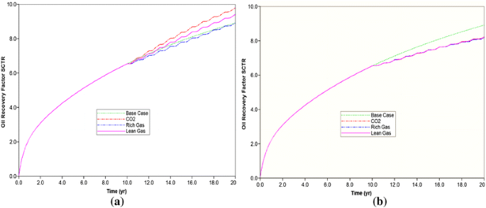

  

  Miscible gases performance in Bakken model for the 1st scenario. a Molar diffusion mechanism is ON. b Molar diffusion mechanism is OFF

The second case of this scenario is exactly the same of the first case for this scenario. However, the molar diffusion mechanism is switched off in the second case while switched on in the first case. The three different miscible gases have been also injected. All the gases have approximately shown the same performance. Their performance is worse than the base case, natural depletion case, because the obtained increment in oil recovery due to the EOR process does not fully upset the loss in oil production during the injection and soaking periods as shown in Fig. 10b.

The results of this scenario are very well consistent with the results which have been reported by Hoteit and Firoozabadi (2009) as shown in Figs. 11 and 12. In their model, which has been conducted in conventional fractured reservoirs, they observed that methane would perform better than CO₂ in the cases which have not considered the molecular diffusion mechanism. However, the injected CO₂ would result in higher increment for oil recovery in the cases which have considered the molecular diffusion mechanism.

$${\text{Rate of Diffusion}} = \frac{{C_{\text{D}} \times \left( {C_{1} - C_{2} } \right) \times {\text{Ac}}}}{{t_{\text{c}} }}$$

(2)

where C _D is the molecular diffusion rate (0.0008–0.0004 cm²/s was specified in this model), (C ₁–C ₂) is the component-concentration difference between the injected fluid and the target fluid, Ac is the contact area between the injected fluid and the target fluid, and t_C is the separation distance between the injected fluid and the target fluid.

Fig. 11

Effect of molecular diffusion on CO₂-EOR performance: a CO₂ performance in shale oil reservoirs—Bakken model, b CO₂ performance in fractured conventional reservoirs (Hoteit and Firoozabadi 2009)

Fig. 12

Effect of molecular diffusion on natural gas-EOR performance: a natural gas performance in shale oil reservoirs—Bakken model, b NG performance in conventional fractured reservoirs (Hoteit and Firoozabadi 2009)

• Second Scenario (2 cycles): This scenario has two cases. In the first case, the molecular diffusion mechanism is switched on and three different miscible gases which are rich gas, lean gas, and CO₂ have been injected. Two cycles have been injected during 10 years. Each cycle injected 500 Mscf/day for 6 months with a soaking period of 3 months. The results indicated that CO₂ performance is the best as compared with lean gas and rich gas. We notice the performance of miscible gases from the best to the worst as CO₂, rich gas, and lean gas, respectively, as shown in Fig. 13a. Interestingly, the rich gas performance exceeds the performance of lean gas in the 2nd scenario while the lean gas performance exceeds rich gas performance in the 1st scenario. The first case of both scenarios is the same; however, the soaking period in this scenario is longer than the soaking period in the previous scenario which favors rich gas on lean gas. The rich gas is showing a good functionality for soaking period as compared with lean gas. This happens due to the difference in the concentration gradient of the miscible gas between the injected fluid and the formation fluid according to Eq. 2 which favors rich gas on lean gas, but rich gas needs a longer soaking period due to its larger molecular weight.

  Fig. 13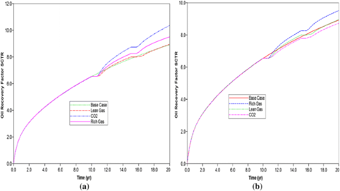

  

  Miscible gases performance in Bakken model for the 2nd scenario. a Molar diffusion mechanism is ON. b Molar diffusion mechanism is OFF

The second case of this scenario is exactly the same of the first case for this scenario. However, the molar diffusion mechanism is switched off in the second case while switched on in the first case. The three different miscible gases have been also injected. The results indicated that rich gas performance is the best as compared to CO₂ and lean gas as shown in Fig. 13b. We notice the performance of miscible gases from the best to the worst as rich gas, lean gas, and CO_2, respectively. The CO₂ has the worse performance in this case. This happens mainly due to the large molecules for CO₂ as compared with lean gas and rich gas. CO₂ would not penetrate into matrix far away from hydraulic fractures if the molecular diffusion rate is low according to Eq. 2 and as shown in Figs. 14 and 15. However, the lean gas and rich gas penetrate deeper into the matrix as compared to what happens in CO₂ injection. This happens in all cases in which the molecular diffusion mechanism is switched off.

Fig. 14

Gas saturation distribution in matrix versus fracture (molar diffusion mechanism is OFF). a Lean gas. b CO₂

Fig. 15

Effect of the injected gas on oil viscosity (molar diffusion mechanism is OFF). a Natural gas, b CO₂

• Third Scenario (Large Volumes Injected): This scenario has four cases. In the first case, the molecular diffusion mechanism is switched on and the three different miscible gases have been injected. Two cycles have been injected during 10 years. Each cycle injected 1500 Mscf/day for 6 months with a soaking period of 3 months. The results indicated that rich gas performance is the best as compared with lean gas and CO₂ as shown in Fig. 16a. We notice the performance of miscible gases from the best to the worst as rich gas, CO₂, and lean gas, respectively.

  Fig. 16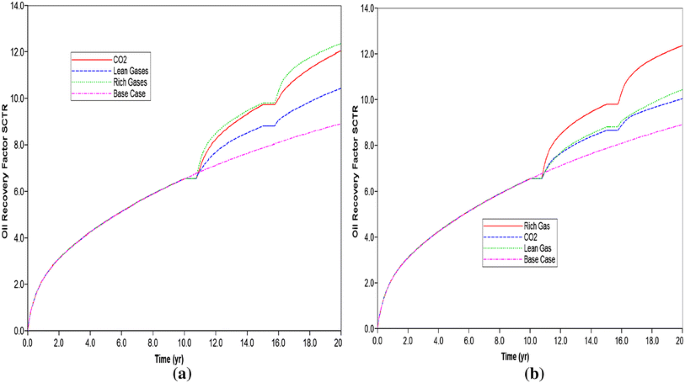

  

  Miscible gases performance in Bakken model for the 3rd scenario. a Case 1, b Case2

The second case is exactly the same of the first case, but the molecular diffusion mechanism is switched off. The results indicated that rich gas performance is the best as compared with lean gas and CO₂ as shown in Fig. 16b. We notice the performance of miscible gases from the best to the worst as rich gas, lean gas, and CO_2, respectively.

In the third case, the molecular diffusion mechanism is switched back on again and the three different miscible gases have been injected. However, in this case, ten cycles have been injected during 10 years. Each cycle injected 1500 Mscf/day for 2 months with a soaking period of 1 month. The results indicated that as far as the molar diffusion mechanism is switched on, CO₂ performance exceeds the performance for both of lean gas and rich gas as shown in Fig. 17a. We notice the performance of miscible gases from the best to the worst as CO₂, lean gas, and rich gas, respectively.

Fig. 17

Miscible gases performance in Bakken model for the 3rd scenario. a Case 3, b Case 4

The fourth case is exactly the same of the third case. However, the molecular diffusion mechanism is switched off. The results indicated that as far as the molar diffusion mechanism is switched off and large volumes injected, lean gas is the best as shown in Fig. 17b. We notice the performance of miscible gases from the best to the worst as lean gas, rich gas, and CO₂, respectively. Figure 18 summarizes the applicability of the three different miscible gases to enhance oil recovery in Bakken Model.

Fig. 18

Applicability of miscible gases EOR in Bakken model

Molar-diffusivity level in the real conditions for shale oil reservoirs

Hoffman and Evans (2016) reported seven pilot tests in Bakken formation which was conducted in North Dakota and Montana. We are presenting only one pilot of them in this section. This pilot was mentioned in his paper as pilot test #2. This pilot test injected CO₂ as huff-n-puff process in Bakken formation, in Montana portion. They injected 1500–2000 Mscf/day of CO₂ for 45 days at 2000–3000 psi. The soaking period was proposed to be 2 weeks. Then, the well was put back in the production process. In puff process, the oil rate had increased slightly above the value which was observed before CO₂ injection, but this increment in oil production rate does not reimburse the oil production lost during the injection and soaking times as shown in Fig. 19.

Fig. 19

a CO₂ pilot test#2 (Hoffman and Evans 2016). b History match from the simulated model

We used the typical fluid and rock properties of Bakken to build a model for that well. Different scenarios have been run until the best match obtained between the well model and the pilot test as shown in Fig. 19. Everything was identical between the model results and pilot test results which are shown in Fig. 19. However, there is only one difference. This difference is that the oil production came quickly after the soaking period in the pilot test; however, it takes longer time in the model case. We believe this is happening due to the reported conformance problems in these pilots where CO₂ produced in the offset wells. Furthermore, we believe that the conformance problems which were happening in those pilots are due to injection-induced fractures (Alfarge et al. 2017). Therefore, the produced-back CO₂ volumes in the production well were small which resulted in less hold up effect on produced oil. However, in our model, we have not induced injection fractures. Therefore, CO₂ in large volumes produced back during the puff process of our model.

Among different scenarios which we investigate, we found that this match can be obtained in a dual-permeability model with low CO₂ molecular diffusivity. This means due to that either of diffusion rate for CO₂ in reservoir conditions is too low or kinetics of oil recovery process in the production areas overcomes the CO₂ diffusivity. The first possibility which is the low diffusivity for CO₂ in shale reservoirs conditions can be explained by two ways: (1) The contact area between the injected CO₂ and formation oil is small (2) The exposure time between the injected CO₂ and the formation oil is short. The contact area between CO₂ and formation oil is mainly a function of natural fractures intensity in shale oil reservoirs. Although it has been reported these types of reservoirs has high intensity of natural fractures, the dual-permeability model can match the conducted pilot test results even with low intensity of natural fractures. This indicated that either of these natural fractures is not active or they are not connected in good pathways with hydraulic fractures.

Closing remarks

Most of the experimental studies reported that CO₂ diffusion mechanism is beyond the increment in oil recovery which was obtained in laboratory conditions. This increment in oil recovery and/or the diffusion rate which were observed in laboratory conditions were upscaled directly by most of the previous researchers to the field scale by using numerical simulation methods. This direct upscaling methodology is so optimistic due to that the laboratory cores have higher contact area and longer exposure time to CO₂ than what happened in the real reservoirs conditions. Therefore, both of simulation studies and experimental works were optimistic to predict a quick improvement in oil recovery from injecting CO₂ in these unconventional reservoirs. This might explain why the results from pilot tests which were using CO₂ as injectant are disappointing and the results from pilot tests which were using natural gases are encouraging (Alfarge et al. 2017). To sum up, diffusion mechanism for CO₂ in pilot tests had not been well recognized, which in turn, did not enhance oil production rate in those wells. The reason beyond the low-diffusion rate for CO₂ in pilot tests is due to either of the kinetics of oil recovery process in productive areas of these reservoirs are too fast or CO₂ diffusion rate in field conditions is too slow (Alfarge et al. 2017). To sum up, the success of CO₂ in shale reservoirs is mainly depending on understanding its main mechanisms which are totally different from its mechanisms in conventional reservoirs. Although most of unconventional IOR studies investigated the applicability of CO₂, they did not properly investigate its soul mechanism in field scale.

Conclusions

• Although most of the previous studies in this area recommended that CO₂ would be the best EOR technique to improve oil recovery in this formation, pilot tests showed that natural gases performance clearly exceeds the CO₂ results in field scale.

• In this study, Péclet number calculations report a significant flow-type heterogeneity in shale reservoirs. However, diffusion flow is the most dominant.

• The simulation results approved that the molecular diffusion has a significant role on EOR by gas injection in Bakken shale reservoir. However, CO₂ needs a good molar-diffusivity into formation oil, so it can enhance oil production in these shale reservoirs. Lean gas and rich gas success requires less molar-diffusivity as compared with CO₂.

• Some of CO₂ pilot tests showed a good match with the simulated cases which have low diffusivity between formation oil and the injected CO₂.

• If the well or field conditions predict a low molar-diffusivity for the injected gases, the rich and lean gases would have a better feasibility than CO₂. However, rich gases need long soaking periods and lean gases need large volumes to be injected for more successful results.

References

Alfarge D, Wei M, Bai B (2017) IOR methods in unconventional reservoirs of North America: comprehensive review. SPE-185640-MS prepared for presentation at the SPE western regional meeting held in Bakersfield, California, USA, 23–27 Apr 2017
Alharthy N, Teklu T, Kazemi H et al (2015) Enhanced Oil Recovery in liquidrich shale reservoirs: laboratory to field. Soc Petrol Eng. doi:10.2118/175034MS
Alvarez JO, Schechter DS (2016) Altering wettability in Bakken shale by surfactant additives and potential of improving oil recovery during injection of completion fluids. Soc Petrol Eng. doi:10.2118/SPE-179688-MS
Clark AJ (2009) Determination of recovery factor in the Bakken formation. Society of Petroleum Engineers, Mountrail County, ND. doi:10.2118/133719-STU
Computer Modeling Group, GEM Manual. www.CMG.Ca/. Accessed 2017
da Silva FV, Belery P (1989) Molecular diffusion in naturally fractured reservoirs: a decisive recovery mechanism. Presented at the SPE annual technical conference and exhibition, San Antonio, Texas, USA, 8–11 Oct. SPE-19672-MS. doi:10.2118/19672-MS
Hawthorne SB, Gorecki CD, Sorensen JA, Steadman EN, Harju JA, Melzer S (2013) Hydrocarbon mobilization mechanisms from upper, middle, and lower Bakken reservoir rocks exposed to CO. Soc Petrol Eng. doi:10.2118/167200-MS
Hawthorne SB, et al (2017) Measured crude oil MMPs with pure and mixed CO2, methane, and ethane, and their relevance to enhanced oil recovery from middle Bakken and Bakken shales. SPE-185072-MS paper was prepared for presentation at the SPE Unconventional Resources Conference held in Calgary, Alberta, Canada, 15–16 Feb 2017
Hoffman BT, Evans J (2016) Improved oil recovery IOR pilot projects in the Bakken formation. SPE-180270-MS paper presented at the SPE Low Perm Symposium held in Denver, Colorado, USA, 5–6 May 2016
Hoteit H, Firoozabadi A (2009) Numerical modeling of diffusion in fractured media for gas-injection and recycling schemes. SPE J. 14(02): 323–337. SPE-103292-PA. doi:10.2118/103292-PA
Kathel P, Mohanty KK (2013) Eor in tight oil reservoirs through wettability alteration. Soc Petrol Eng. doi:10.2118/166281MS
LeFever J, Helms L (2008) Bakken formation reserve estimates, North Dakota Geological Survey. https://pdfs.semanticscholar.org/107e/8bba008ec7333360a067b49fbb76b2a44caf.pdf
Mohebbinia S, et al (2017) Molecular diffusion calculations in simulation of gasfloods in fractured reservoirs. SPE-182594-MS paper presented at the SPE reservoir simulation conference held in montgomery, TX, USA, 20–22 Feb 2017
Moortgat J, Firoozabadi A (2013) Fickian diffusion in discrete-fractured media from chemical potential gradients and comparison to experiment. Energy Fuel 27(10):5793–5805. doi:10.1021/ef401141q
Schmidt M, Sekar BK (2014) Innovative unconventional 2EOR-A light EOR an unconventional tertiary recovery approach to an unconventional Bakken reservoir in Southeast Saskatchewan. World Petroleum Congress
Sheng JJ (2015) Enhanced oil recovery in shale reservoirs by gas injection. J Nat Gas Sci Eng 22:252–259. doi:10.1016/j.jngse.2014.12.002
Wan T, Sheng J (2015) Compositional modelling of the diffusion effect on EOR process in fractured shale-oil reservoirs by gasflooding. Soc Petrol Eng. doi:10.2118/2014-1891403-PA
Wang D, Zhang J, Butler R, Olatunji K (2016) Scaling laboratory-data surfactant-imbibition rates to the field in fractured-shale formations. Soc Petrol Eng. doi:10.2118/178489-PA
Wood T, Milne B (2011) Waterflood potential could unlock billions of barrels: Crescent Point Energy. http://www.investorvillage.com/uploads/44821/files/CPGdundee.pdf
Yu W, Lashgari H, Sepehrnoori K (2014) Simulation study of CO2 Huff-n-Puff process in Bakken tight oil reservoirs. Society of Petroleum Engineers. doi:10.2118/169575-MS
Yu Y, Li L, Sheng J (2016) Further discuss the roles of soaking time and pressure depletion rate in gas Huff-n-Puff process in fractured liquid-rich shale reservoirs. SPE-181471-MS paper presented in at the SPE annual technical conference and exhibition held in Dubai, UAE, 26–28 Sept 2016
Zhang K (2016) Experimental and numerical investigation of oil recovery from Bakken formation by miscible CO2 injection. Paper SPE 184486 presented at the SPE international student paper contest at the SPE annual technical conference and exhibition held in Dubai, UAE, 26–8 Sept 2016
Author information
Authors and Affiliations
Corresponding author
Rights and permissions
Open Access This article is distributed under the terms of the Creative Commons Attribution 4.0 International License (http://creativecommons.org/licenses/by/4.0/), which permits unrestricted use, distribution, and reproduction in any medium, provided you give appropriate credit to the original author(s) and the source, provide a link to the Creative Commons license, and indicate if changes were made.
About this article
Cite this article
Alfarge, D., Wei, M. & Bai, B. Numerical simulation study on miscible EOR techniques for improving oil recovery in shale oil reservoirs. J Petrol Explor Prod Technol 8, 901–916 (2018). https://doi.org/10.1007/s13202-017-0382-7
Received:
Accepted:
Published:
Issue Date:
DOI: https://doi.org/10.1007/s13202-017-0382-7