Real-time water quality monitoring through Internet of Things and ANOVA-based analysis: a case study on river Krishna

Abstract

In this paper, an attempt has been made to develop a statistical model based on Internet of Things (IoT) for water quality analysis of river Krishna using different water quality parameters such as pH, conductivity, dissolved oxygen, temperature, biochemical oxygen demand, total dissolved solids and conductivity. These parameters are very important to assess the water quality of the river. The water quality data were collected from six stations of river Krishna in the state of Karnataka. River Krishna is the fourth largest river in India with approximately 1400 km of length and flows from its origin toward Bay of Bengal. In our study, we have considered only stretch of river Krishna flowing in state of Karnataka, i.e., length of about 483 km. In recent years, the mineral-rich river basin is subjected to rapid industrialization, thus polluting the river basin. The river water is bound to get polluted from various pollutants such as the urban waste water, agricultural waste and industrial waste, thus making it unusable for anthropogenic activities. The traditional manual technique that is under use is a very slow process. It requires staff to collect the water samples from the site and take them to the laboratory and then perform the analysis on various water parameters which is costly and time-consuming process. The timely information about water quality is thus unavailable to the people in the river basin area. This creates a perfect opportunity for swift real-time water quality check through analysis of water samples collected from the river Krishna. IoT is one of the ways with which real-time monitoring of water quality of river Krishna can be done in quick time. In this paper, we have emphasized on IoT-based water quality monitoring by applying the statistical analysis for the data collected from the river Krishna. One-way analysis of variance (ANOVA) and two-way ANOVA were applied for the data collected, and found that one-way ANOVA was more effective in carrying out water quality analysis. The hypotheses that are drawn using ANOVA were used for water quality analysis. Further, these analyses can be used to train the IoT system so that it can take the decision whenever there is abnormal change in the reading of any of the water quality parameters.

Introduction

In the world, and especially in India, river water is the main source for all anthropogenic activities such as drinking, irrigation and agriculture (Parmar and Bhardwaj 2014; Herojeet et al. 2016).The river water quality is getting degraded day by day, and water pollution is the main reason for degradation in the recent years. The water is getting polluted mainly because of rapid industrialization of river basins and river Krishna is also one among them. River Krishna has rich mineral deposits, which makes it best suited for industrial development. The different industries that are active in the river Krishna basin region are sugar, cement, iron and steel, vegetable oil extraction and rice mills (Central Water Commission 2014). These industries produce the wastes such as (a) dirt and gravel, (b) masonry and concrete, (c) scrap metals, (d) trash, (e) oil, (f) chemicals, (g) effluents and suspended solids and (h) organic matters. These pollutants alter the physio-chemical characteristics of aquatic ecosystem because it has high concentration of BOD and TDS which cause rapid depletion of oxygen in water. It is estimated that every year, millions of tons of waste in the form of industrial waste, agricultural waste and urban waste water is dumped into the river, thus making the water from the river unusable and requires frequent quality checks (Shah and Joshi 2017; Kaur et al. 2017; Parmar and Bhardwaj 2014; Loganathan and Ahamed 2017). In India, the water quality check is carried under the careful monitoring of Central Pollution Control Board (CPCB) (Nagar 2007). All the rivers including river Krishna is monitored under Monitoring of Indian National Aquatic Resource System (MINARS) (Central Pollution Control Board 2013).

The parameters considered to carry out the water quality analysis of river Krishna were pH, TDS, turbidity, DO, temperature, conductivity, nitrate and BOD(Yan et al. 2014; Huang 2012; Verma and Prachi 2012; Jiang et al. 2009; Yunbing 2013; Geetha and Gouthami 2016; Wang et al. 2013). Table 1 shows the brief description of each parameter. The technique to assess the quality is still traditional and manual, i.e., collecting the sample from the site and taking it to the laboratory for investigation, which is a time-consuming activity. The people in the river basin region are deprived of real-time water quality alerts. Hence, IoT-based real-time system is the solution.

Table 1 The water parameters

IoT is basically a real-time remote sensing communication system, where devices are deployed at the sampling site of river Krishna to monitor the water quality. The different sensors collect data at frequent time intervals and send the same to the data center for statistical analysis.

The statistical model used in this work is based on one-way and two-way analysis of variance (ANOVA). The results obtained from the work can be fed back to the system (Tiri et al. 2015). Hence, action can be taken immediately, whenever abnormality in the data is observed, further. In this study, we have chosen river Krishna in the state of Karnataka region because previous studies were carried out in either Maharashtra part of region or Andhra part of region (Kengnal et al. 2015; River and Initiative 2014; Water et al. 2000). The present work is undertaken in order to monitor the water quality of river Krishna using ANOVA-based real-time IoT system.

A model was developed to test the water quality of the samples collected from the pipeline using IoT system. The data collected is than stored in cloud storage for future analysis. The IoT systems also alert the user whenever there is a variation in the parameter readings from a predefined standard values (Geetha and Gouthami 2016).

An online water quality management system (OWQMS) was developed to study the urban river in china as a part of environmental Internet of Things (EIoT). OWQMS has three main components: (a) multiparameter water quality analyzer, (b) an information transmission system and (c) a computer system unit. The pollutants such as organic and nitrogen, phosphorus contents were measured manually and analyzed using water quality parameters such as pH, DO, turbidity, conductivity, oxidation–reduction potential (ORP), chlorophyll, temperature and salinity of the water. Depending on the results, the water was purified. After purification, all the parameters reached the prescribed standards. River cycling was the method used for purification of river water (Wang et al. 2013).

Two-way ANOVA is used for water quality assessment on parameters such as pH, TDS, DO and BOD, which shows that there is huge deterioration of water quality at the sites near the urban settlements in Malaysian peninsular region. It also emphasized that the side channels of Malaysian peninsular were more polluted than the main stream river. Therefore, a periodic check on the parameters will help in the remedial measures in order to check the oxygen depletion (VishnuRadhan et al. 2017).

Weighted arithmetic water quality index method that provides a single number (like a grade) that expresses overall water quality at a certain location and time based on several water quality parameters was used to check the quality of water in Sabarmati River. The advantages of this method are: (a) It uses multiple parameters (pH, DO, chloride, coliforms) data to formulate mathematical equation that checks the health of water. (b) Weightage of each parameter decides the unit weight of each indicator parameter, which is used to calculate the sub-index value. (c) It shows the composite influence of each parameter on water quality management. (d) These sub-indices values were then used to determine overall water quality index (WQI). WQI is a rating technique used to check the overall water quality as a single term. It is useful in selection of appropriate treatment technique to solve the concerned issue (Shah and Joshi 2017).

A combination of hierarchical cluster analysis (HCA) and ANOVA is used to study the water quality at Koudiat Medouar, East Algeria. This study found that the water in this area was alkaline, so electrical conductivity was high. All the parameters Mg, Ca, HCO₃ and SO₄ were considered significant in quality analysis determination at observing station 1. Electrical conductivity was vital parameter in observing station 2, and parameters pH and NO₃ were critical parameters for quality analysis in observing station 3 (Tiri et al. 2015).

The quality of river Yamuna in Delhi was observed using the water quality index technique (WQI) for pre-monsoon, monsoon and post-monsoon seasons at 4 different locations in Delhi. It was found that the water quality was marginally good to very poor in study area, and the parameters that were critical in the observations were BOD, DO, total and fecal coliforms and free ammonia. WQI factors are used in combination to get a number between 0 and 100 which is used to assess the water quality of river Yamuna (Sharma and Kansal 2011).

The quality of water was assessed by hydro-chemical analysis using water quality analyzer in accordance with American Public Health Association (APHA). The water quality analysis was carried out on all rivers flowing in Malwa region in Punjab, India. In this analysis, it was found that pH was in permissible limits prescribed by WHO standards, but water had a high turbidity, which means that water contained high-level disease causing organism such as viruses, bacteria and parasites that can cause nausea, cramps and diarrhea. It was also found that the water was hard and alkaline, i.e., the pH was much higher than the permissible standards prescribed by WHO. It was found that the use of fertilizers with iron, phosphate and ammonium ions contents was the main reason for source of arsenic content in some of the water analysis sites (Kaur et al. 2017).

Statistical analysis of water quality was done using time series prediction model. This model makes use of autoregressive integrated moving average (ARIMA), R-square, root mean square error (RMSE), mean absolute percentage error (MAPE), mean absolute error (MAE) and normalized Bayesian information criterion (BIC) to find out the water quality of river Yamuna. In this analysis, it was found that water was unfit to use for drinking and agricultural purpose because it was found that the pH and water temperature (WT) parameter levels were exceeding the WHO standards limits (Parmar and Bhardwaj 2014).

Fuzzy Comprehensive analysis is used to quantify the factors with unclear boundary using fuzzy mathematics that uses a form of logic based on the concept of a fuzzy set to evaluate water quality. System Cluster analysis is also used to evaluate the water quality of rivers, i.e., one cluster is evaluated and is combined with another cluster with similar characteristics, and this process is repeated until all clusters are combined together into one cluster. Usually, the cluster analysis is based on geographical location and date (Xu et al. 2012).

Principal component analysis (PCA) and cluster analysis (CA) techniques were used for water quality analysis study. PCA provides information of most important parameters such as temperature, pH, electrical conductivity (EC) and DO and is used in statistical correlation. It uses pattern recognition technique to get variance in large set of inter-correlated variables. It also uses CA to group parameters into one group with similar characteristics. Hierarchical agglomerative clustering is a “bottom-up” approach and was used to normalize data (Zhao et al. 2012).

Factor analysis technique along with PCA was applied on the samples collected from different sources like tube-well, open-well and hand pumps. Mainly two factors are identified as the factors for variation in water quality, i.e., (a) anthropogenic sources and (b) organic source. The parameters which are affected by anthropogenic factors are electrical conductivity (EC), total dissolved solids (TDS), calcium hardness, (Ca-H), magnesium hardness (mg-H), total hardness, (TH), chloride (CL −), alkalinity, sodium (Na +), potassium (K +) and nitrate (NO3). The parameter that was affected was pH, and the organic factor affecting the water quality was presence of fluoride content in the surface water (Kumar et al. 2010).

The combination of three multivariate statistical techniques such as CA, factor analysis (FA) and PCA was used to find out the water quality of river Haraz in Iran. According to CA, the river can be divided into three clusters: low, moderate and high pollution clusters. PCA is used to identify the variations in the water quality in different seasons. Factor analysis is used to lessen the number of variables and discover the structure in relationship between different variables. The parameters that were affecting the water quality were temperature, TDS and NO₃. It was also found that parameter affecting water quality in one season may not be a factor of significance in another season (Pejman et al. 2009).

The analysis was carried out using envirometric techniques such as PCA, CA and WQI in the industrial area of Baddi Barotiwala Nalagarh, Himachal Pradesh, India. Water samples were collected from different sources such as tube-well, dug-well, well and spring for water analysis and were compared with the Bureau of Indian Standards (BIS) for its correctness. According to WQI analysis, 93.76% of water in pre-monsoon and 81.25% of water in post-monsoon seasons were found to be not suitable for human consumption. Then, PCA was applied on the same dataset and was found that 80.1% and 75.7% of total variance was observed in pre-monsoon and post-monsoon analysis. CA was used to identify the similar groups between different sampling points for pre-monsoon and post-monsoon season. All samples were clustered into four clusters for both pre-monsoon and post-monsoon. It was found that pre-monsoon clusters were affected by both natural and anthropogenic source, but the main contributor for pollution was anthropogenic source. Though the post-monsoon was also affected by natural and anthropogenic sources, the main pollutant was natural source (Herojeet et al. 2016).

WQI analysis using artificial neural network (ANN) was used for prediction of water quality. ANN algorithms applied are: (i) Early stopping: uses three data subsets, the first is a training subset used for computing and updating the gradients, network weights and biases. The second subset is a validation subset which is used to monitor errors during training. And last subset was used to obtain the maximum hidden nodes, (ii) Ensemble: used in neural network to deal with noisy data or small data sets, and to train multiple neural networks and average their outputs, (iii) Bayesian regularization: used to solve over-fitting problem. It uses goodness to fit and network architecture to minimize the problem. This method is used for modifying some of the objective functions such as mean square error (MSE) with aim to improve the model’s generalization capability. It was seen that performance of Bayesian regularization method was better than the other two methods in predicting WQI followed by ensemble and early stopping (Sakizadeh 2016).

A combination of three different multivariate statistical analyses, namely PCA, discriminant analysis (DA) and general linear model (GLM), was used to assess the water quality. After applying PCA to the datasets, it was observed that natural sources of pollution were affecting most of the parameters of water. DA was then applied in three steps, namely: (a) Standard: All water quality parameters enter the model simultaneously. (b) Forward: The variables enter the model in successive steps. At each step, large significant value of variable is chosen for inclusion in the model. (c) Backward steps: All the variables are included into the model, and then in each step, variable with least significant value is eliminated. DA is useful in removing effects of different measurement units for standardized variables. The GLM was used to study the effects of high and low flows on surface water quality. Thus, differences in the water quality were detected for both low and high flow. The study suggested that parameters that affect water quality during low flow may not be the same during the high flow (Nosrati 2015).

HCA was performed on different water parameters based on the similarities of different cluster, with the aim to get an optimal cluster. Then, multiple linear regression (MLR) was applied which quantifies the relationship between independent variables with dependent variables. MLR was essential to find out the relationship between depth of siltation and water quality parameters. Lastly, mathematical equation modeling (MEM) was applied and was found that the water parameters such as temperature, salinity, pH, DO and conductivity along with depth of siltation were affecting the water quality. The degradation of water quality was mainly due to agricultural waste, soil erosion and tidal effect in the area. It was found that as the siltation increases, the water quality starts degrading (Roy et al. 2014).

Multivariate statistical analysis such as hierarchical cluster analysis (HCA) and principal component analysis (PCA) along with Karl Pearson Correlation Matrix Analysis (KPCMA) was employed to determine the water quality of river Amaravathi, India. PCA was applied on large data set, for data reduction and deciphering the patterns within the dataset in order to provide information about the most important and meaningful parameters. HCA is used as the classification technique. HCA uses two techniques, namely Q-mode and R-mode analysis. The samples are classified into distinct hydro-chemical groups using Q-mode. Similarly, the linking of variables were carried out using R-mode. KPCMA is basically a hydro-chemical study that specifies the association between individual parameters along with various factors controlling it. It was found from the study that EC, TDS, pH, DO and BOD parameters were mainly affected by anthropogenic activity in the region (Loganathan and Ahamed 2017).

Materials and methods

Study area

The origins of river Krishna is in the state of Maharashtra at the village called Jor near Mahabaleshwar in Satara district at the coordinate points of 17°59′18.8″N latitude, 73°38′16.7″E longitude at an elevation of 1372 m. The river flows eastwards passing through the states of Karnataka, Telangana and Andhra Pradesh to finally reach the Bay of Bengal. Our area of study deals only with the part of river Krishna that flows through the state of Karnataka. The river Krishna enters the state of Karnataka near village Jugala at the coordinate points of 16°37′16.64″N latitude, 74°41′29.06″E longitude and flows approximately about 483 km in state of Karnataka (Fig. 1).

Fig. 1

Source: Krishna Basin Profile published by Central Water Commission and google map)

River Krishna basin and details of water collecting stations

Sampling

Table 2 shows the stations from which the samples were collected and these stations are standard locations taken from national database; a total of 36 samples, i.e., six samples per station, were collected randomly. Out of six samples collected from each station, a pair of samples represents the summer, rainy and winter season, respectively. The stations in Karnataka regions are as follows:

Table 2 Water sample collection stations in Karnataka

IoT system specification

Internet of Things (IoT) is nothing but making the real physical objects to talk to each other using internet. It is the capability of things to sense, communicate, interact and collaborate with other things using embedded technology, by creating a network of physical objects. IoT could be a system of interconnected computing devices, mechanical and digital machines, objects, animals or those who are given distinctive identifiers and also the ability to transfer knowledge over a network while not requiring human-to-human or human-to-computer interaction. Figure 2 shows Internet of Things (IoT) test bed for measuring the different water quality parameters to collect the samples. Our test bed comprises of the following:

Fig. 2

The circuit and the block diagram of IoT system

Arduino Mega 2560

The Arduino Mega 2560 is a microcontroller board based on the AT mega 2560. It has 54 digital input/production personal identification number (of which fourteen can be used as PWM outputs), sixteen analog inputs, 4 UARTs (hardware serial port), a 16 Megacycle per second crystal oscillator, a USB connection, a major power jack, an ICSP coping and a reset button. It contains support in the form of microcontroller, simply connect it to a computer with a USB cable or power it with an AC-to-DC adapter or a battery to get started.

pH sensor

Water pH is the measure of concentration of H + ions in the water. As water pH decreases, it becomes more acidic and as the number of H + ions increases, it becomes more alkaline. The AWQMP is designed to use YSI pH 6-series sensors (YSI 2013) for pH measurements. The sensors can handle all ionic strength conditions, from seawater, to “average” freshwater lakes and rivers, to pure mountain streams. The sensors specifications are: a range of 0–14 units with resolution of 0.01 units and accuracy of ± 0.1 unit.

Temperature sensor

Temperature sensor is used to measure the temperature of H₂O. It is one of the most important parameters to be considered. It dramatically affects the rates of chemical substance and biochemical reactions within water. Many biological, physical and chemical principles are temperature dependent. The most common are: the solvability of compound in sea water; distribution and abundance of organisms aliveness in the watershed; rates of chemical reactions; water density; inversion and mixing; and current campaign.

Dissolved oxygen sensor

The dissolved oxygen sensor output is 4–20 mA with a three wire configurations. The dissolved oxygen sensor’s electronics are completely encapsulated in marine grade epoxy within stainless steel housing. The dissolved oxygen sensor uses a removable shield and dissolved oxygen element for easy maintenance.

Biochemical oxygen demand

BOD detector systems comprise of a six position stirring units complete with 6 BOD Sensor, 6 alkali holder for absorbing the carbon dioxide and 6 stirring bars. This instrument is a complete solution for the user. It is immediately operational for measuring the BOD with 4 exfoliation—XC, 250, 600 and 999 ppm BOD—or higher value after dilution.

Conductivity sensor

Conduction sensor is suitable for measurement conduction in a wide variety of covering including science laboratory, streams, rivers and groundwater. The conductivity detector’s small size and rugged housing shuffle are useful for hand-held mensuration or permanent installation. The conductivity sensors use a 4-electrode mensuration technique that provides accurate readings over a wide range of conduction and temperatures. An in-bloodline interface module converts the digital conductivity sensor and temperature data into two separate 4–20 mA signals for monitoring with data logger and PLC devices.

Esp8266

ESP8266 is an impressive, low-cost WiFi unit suitable for adding WiFi functionality to an existing microcontroller task via a UART serial connection. The module can even be reprogrammed to act as a standalone WiFi-connected device.

Statistical methods

In our work, we have used one-way ANOVA and two-way ANOVA for water quality analysis. The ANOVA was applied on the collected dataset. The brief description of one-way ANOVA and two-way ANOVA is given below.

One-way ANOVA

Analysis of variance (ANOVA) is associate degree analysis tool employed in statistics that splits the combination variability found within a knowledge set into 2 parts: systematic factors and random factors. The systematic factors have an applied mathematics influence on the given information set; however, the random factors do not. ANOVA may be a cluster of statistical models to check if there exists a major distinction between means. It tests whether or not the means that of varied group is equal or not. In ANOVA, the variance observed in particular variable is partitioned off into totally different element based on the sources of variations. We use multivariate analysis to check out whether or not the means differ considerably. The ANOVA produces an F-statistic, the ratio of the variance calculated among the means to the variance within the samples.

$$F = {\text{variation between sample means }}/{\text{variation within the samples}}$$

$$F{\text{ - critical}}\left( {0.05} \right) = \frac{{{\text{Variance}}1}}{{{\text{Variance}}2}}$$

$$R2 = 1 - {\text{SSE /SST}}$$

$$R2\quad {\text{adj }} = 1 - {\text{MSE /MST}}$$

$$P{\text{-value }} = 2 *P ({\text{TS}} \ge \left| {\text{ts}} \right| |H0 {\text{is true}}) = 2 * \left( {1 - {\text{cdf}}\left( {\left| {\text{ts}} \right|} \right)} \right)$$

Two-way ANOVA

It is an extension of the one-way analysis of variance that examines the influence of 2 totally different categorical independent variables on one continuous variable. The two-way analysis of variance not solely aims at assessing the main impact of every experimental variable, however, even if there is any interaction between them.

The following algorithm and flowchart in Fig. 3 show how we are trying to model our analysis:

Fig. 3

The hypothesis check for prediction

Results

One-way ANOVA results

We apply one-way ANOVA on each of the water parameters, namely temperature, DO, pH, BOD, conductivity, TDS and nitrate. We group these parameters according to the stations at which the samples were collected. We trifurcate our analysis based on three seasons, namely summer season in between March and May, rainy season in between June and August and winter season in between November and January.

Summer season

During summer season, it was observed that the water is either stagnant or water level in the river was low mainly due to evaporation or heavy consumption, and the following observations were made.

• (i) Temperature: The station 1028 has the lowest mean temperature of 32.2 °C, and station 1181 has the largest standard deviation of 3.64 among all stations (Fig. 4a); the mean temperature of 31.33 °C was recorded maximum at station 1170 (Fig. 4b).

  Fig. 4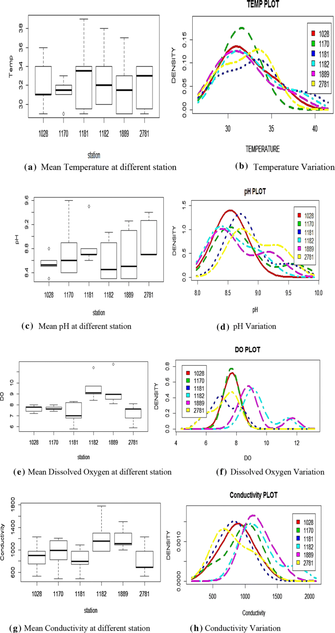

  

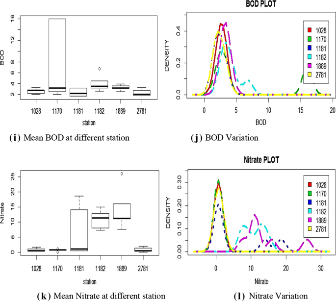
  a Mean temperature at different stations, b temperature variation, c mean pH at different stations, d pH variation, e mean dissolved oxygen at different stations, f dissolved oxygen variation, g mean conductivity at different stations, h conductivity variation, i mean BOD at different stations, j BOD variation, k mean nitrate at different stations, and l nitrate variation

• (ii) pH: The smallest mean pH value of 8.53 was observed at station 1028, and station 1170 had a large standard deviation of 0.364 among all stations (Fig. 4c); the mean pH value of 8.97 was maximum at station 2781 followed by 1181 with value of 8.82 (Fig. 4d).

• (iii) DO: The station 1181 had smallest mean value of 7.18 DO, and station 1889 had the largest standard deviation of 1.0 (Fig. 4e); the mean DO at station 1182 was maximum at 9.4, closely followed by 1889 stations with value of 9.2, respectively (Fig. 4f).

• (iv) Conductivity: It was observed that the smallest mean conductivity value of 814.88 was observed at station 1181, and the largest standard deviation of 298.42 was recorded at station 1182 (Fig. 4g); meanwhile, the maximum conductivity of 1224.88 was recorded at station 1182 (Fig. 4h).

• (v) BOD: The station 2781 had a smallest mean BOD of 2.25, and station 1182 having a largest standard deviation of 1.19 (Fig. 4i); the maximum mean BOD of 4.01 was observed at station 1182 followed by station 1889 with the value of 3.26 (Fig. 4j).

• (vi) NO₃: The station 1170 had the lowest mean nitrate value of 0.6, and station 1889 had the largest standard deviation of 5.17 among all stations (Fig. 4k); the mean Nitrate value of 13.81 was recorded maximum at station 1889 (Fig. 4l).

After applying one-way ANOVA on the dataset for each individual parameter, the following results are obtained from Table 3.

Table 3 One-way ANOVA calculations for summer season

From Table 3 observations, we can conclude that the parameters that were affecting the analyses of water quality are:

• (a) DO: The p value of the parameter 0.000 was less than α value of 0.05, so null hypotheses can be rejected.

• (b) Conductivity: Because the p value of the parameter 0.021 was less than α value of 0.05, null hypotheses can be rejected.

• (c) NO₃: The p value of the parameter 0.000 was less than α value of 0.05, so null hypotheses can be rejected.

This means that DO, conductivity and NO₃ are the parameters that were affecting the water quality in the summer season.

In summer season, it can be observed from Fig. 5 that the conductivity parameter is more prominent due to low water level and more the mineral concentration in water if the conductivity crosses 500 ppm which is not recommended for drinking purpose. Similarly, the pH parameter value was also found to be more. It also shows the station-wise variation of different parameters for year 2008 and year 2016, respectively, and similar observations were made for years 2009–2015. Figure 6 also depicts the summary of total dissolved solids at each station. In the year 2010–2011, in the following stations 1028, 1170, 1181 and 2781, it was observed that the concentration of minerals in the water was less may be due to two possibilities those are (a) on demand release of water from the dams in Maharashtra. (b) due to torrential rains in catchment area of these stations. Similarly in year 2012, station 1182 recorded highest conductivity. In year 2013, station 1189 recorded the highest TDS. It is also observed that from year 2014 onward the conductivity is in the range of 500–700 ppm.

Fig. 5

Yearly variations of different water parameters in summer season for year 2008 and 2016

Fig. 6

Year-wise data of TDS at each station for summer season

Rainy season

During the rainy season, it was observed that the water level in the river was maximum, mainly due to heavy rainfall in the catchment area, as a result the following observations are made from Table 4.

Table 4 One-way ANOVA for rainy season

• (i) Temperature: The station 1182 and 1889 recorded the lowest mean temperature of 23.66 °C, and station 1182 has the largest standard deviation of 1.96 among all stations; the mean temperature value of 27 °C was recorded maximum at station 1170.

• (ii) pH: The lowest mean pH value of 7.51 was observed at stations 2781 and 1181, and probably station 2781 had a largest standard deviation of 0.23 among all stations; the mean pH was maximum value of 7.9 at station 1170 followed by 1182.

• (iii) DO: The station 2781 had smallest mean value of 5.28 DO, and the station 1889 had a largest standard deviation value of 0.54; the mean DO value of 6.87 at station 1028 was at maximum.

• (iv) Conductivity: It was observed that the smallest mean conductivity value of 239.88 was observed at station 1182, and the largest standard deviation value of 90.87 was recorded at station 1170; meanwhile, the maximum conductivity value of 350.88 was recorded at station 1170.

• (v) BOD: The station 1182 had a smallest mean BOD value of 0.5 with station 1181 having a largest standard deviation value of 0.35, and the maximum mean BOD value of 1 was observed at stations 1028 and 1170.

• (vi) NO₃: The stations 1181 and 2781 had the lowest mean nitrate value of 0.02, and station 1182 has the largest standard deviation with value of 2.13 among all stations; the mean Nitrate value of 3.01 was recorded maximum at station 1182.

After applying one-way ANOVA on the dataset for each individual parameter, the following results were obtained.

From Table 4 observations, we can conclude that the parameters that were affecting the analyses of water quality are:

• (a) Temperature: The p value of the parameter 0.001 was less than α value of 0.05, so null hypotheses can be rejected.

• (b) DO: The p value of the parameter 0.000 was less than α value of 0.05, so null hypotheses can be rejected.

• (c) BOD: Because the p value of the parameter 0.020 was less than α value of 0.05, null hypotheses can be rejected.

• (d) NO₃: The p value of the parameter 0.002 was less than α value of 0.05, so null hypotheses can be rejected.

This means that the parameters such as temperature, DO, BOD and NO₃ were affecting the prediction of water quality in rainy season.

In rainy season, the conductivity was under check except for one station, i.e., 1170; DO was the cause of concern because DO depends on temperature which is low. Figure 7 shows the station-wise variation of different parameters for year 2008 and year 2016, respectively, and similar observations were made for years 2009–2015. According to Fig. 8, in year 2008, it was observed that almost all the stations except 2781 had recorded the highest conductivity factor due to less rainfall in the catchment area. Similarly, the TDS was recorded more during the year 2013 again due to less rainfall. Otherwise, all the stations recorded steady values during year 2014 to 2016.

Fig. 7

Yearly variations of different water parameters in rainy season for year 2008 and 2016

Fig. 8

Year-wise data of TDS at each station for rainy season

Winter season

During the winter season, the water level in the river was normal; hence, the following observations were made.

• (i) Temperature: The station 1889 recorded the lowest mean temperature of 26.68 °C, and station 1889 has the largest standard deviation value of 1.28 among all stations; the mean temperature of 28.88 °C was recorded maximum at station 1028.

• (ii) pH: The lowest mean pH value of 8.11 was observed at station 1889, and station 1028 had a large standard deviation of 0.17 among all stations; the mean pH value of 8.3 was maximum at station 1170.

• (iii) DO: The station 2781 had smallest mean DO value of 6.09, and the station 1181 had a largest standard deviation value of 0.66; the mean DO at station 1028 was at maximum with value of 7.3.

• (iv) Conductivity: It was observed that the smallest mean conductivity with value of 547.44 was observed at station 2781, and the largest standard deviation was recorded at station 1170 with the value of 108.69; meanwhile, the maximum conductivity was recorded at stations 1182 with the value of 734.44.

• (v) BOD: The station 1181 had a smallest mean BOD value of 1.39, with station 1170 having a largest standard deviation of the value 0.5; the maximum mean BOD value of 2.40 was observed at station 1170.

• (vi) NO₃: The station 2781 has the lowest mean nitrate value of 0.30, and station 1889 had the largest standard deviation of 4.35 among all stations; the mean nitrate value of 8.18 was recorded maximum at station 1889.

After applying one-way ANOVA on the dataset for each individual parameter, the following results are obtained from Table 5.

Table 5 One-way ANOVA for winter season

From Table 5 observations, we can conclude that the parameters that were affecting the analyses of water quality are:

• (a) Temperature: The p value of the parameter 0.001 was less than α value of 0.05, so null hypotheses can be rejected.

• (b) DO: The p value of the parameter 0.000 was less than α value of 0.05, so null hypotheses can be rejected.

• (c) Conductivity: The p value of the parameter 0.010 was less than α value of 0.05, so null hypotheses can be rejected.

• (d) BOD: The p value of the parameter 0.001 was less than α value of 0.05, so null hypotheses can be rejected.

• (e) Nitrate: Because the p value of the parameter 0.000 was less than α value of 0.05, null hypotheses can be rejected.

This means that in winter season, the parameter that are affecting the prediction of water quality are temperature, DO, conductivity, BOD and Nitrate.

The following Fig. 9 shows the year-wise data of river Krishna from year 2008–2016 (for all three seasons) and station-wise for the parameters like temperature, pH, conductivity, DO, Nitrate, BOD and total dissolved solids (TDS).

Fig. 9

Yearly variations of different water parameters in winter season for year 2008 and 2016

In winter season, we can see that the conductivity parameter is more prominent among the other parameters and ranges between 600 to 800 ppm in water. Similarly, the BOD and DO values were found to be more than normal. Figure 9 shows the station-wise variation of different parameters for year 2008 and year 2016, respectively, and similar observations were made for years 2009–2015. In Fig. 10, we can see that for year 2008, station 1170 had a highest TDS value, while other stations were in the CPCB standard. Similarly for year 2013, stations 1170 and 1889 had conductivity value more than CPCB permissible limits, so it is advisable not to use water for drinking purpose. From 2014 onward, the TDS was in normal range as given by CPCB.

Fig. 10

Year-wise data of TDS at each station for winter season

Two-way ANOVA results

In our statistical analysis, we try and evaluate the effects of water parameters with respect to the observing stations. The following observations are made from Table 6:

Table 6 The two-way ANOVA observation table

• (a) Temperature in summer, rainy and winter in each of the stations: The observation suggests that for sample, there is a significant difference in F and F-critical value and also the P value is very small as compared to alpha value (0.05).

• (b) For columns, though there is no much difference in F and F-critical values, P value is smaller than alpha value.

• (c) The interaction shows that as independent parameter the temperature is not acceptable because there is a huge variation in F value and F-critical values as well as P value; it is acceptable as a group because there is no much difference in F value and F-critical values.

• (d) DO shows that neither as the independent variable nor as a group the prediction cannot be accepted because there is a huge difference between F and F-critical values for sample, for columns nor for interaction; also the P value is much lesser than alpha value.

• (e) pH when considered as only sample: It is not acceptable because there is a huge difference between F and F-critical values; otherwise, it is accepted as columns and interaction as F and F-critical and P value are within range.

• (f) Conductivity parameter is bound to create an exception because all the critical attributes, i.e., F, F-critical and P value are significantly not acceptable.

• (g) BOD as an interaction between sample and columns is only acceptable because F and F-critical values are in acceptable range, otherwise as an independent variables F, F-critical and P value differ significantly.

• (h) NO₃ shows that neither as the independent variable nor as a group, the prediction can be accepted because there is a huge difference between F and F-critical values for sample, columns and interaction; also the P value is much lesser than alpha value.

• (i) TDS shows that neither as the independent variable nor as a group, the prediction can be accepted because there is a huge difference between F and F-critical values for sample, columns and interaction; also the P value is much lesser than alpha value.

Conclusion

An IoT system was developed to monitor river Krishna in real time. The IoT system was used to collect the data from identified stations for different water quality parameters such as pH, turbidity, DO, BOD, NO₃, temperature and conductivity to generate a data set that was used to monitor the quality of water. The collected data were successfully utilized to assess the water quality of river Krishna using one-Way ANOVA which analyze a particular parameter and predict the quality based on value obtained. Two-way ANOVA was used to do the analysis of two parameters as a single entity as well as a combination of two parameters. The results showed that one-Way ANOVA was best suited for training the IoT system. The observations showed that all the water quality parameters play a vital role in one or the other seasons. In summer season, the parameters conductivity and TDS were found to be more concentrated due to low water level in the river and the water quality was 30.39%. In rainy season, the water quality was 65.37% and the parameter affecting the water quality was DO. In winter seasons, DO was the parameter which affected the water quality and the water quality was 46.47%. The collected data set can also be used in future to make the system intelligent by applying machine learning techniques.

References

Central Pollution Control Board (2013) Status of water quality in India 2011. Central Pollution Control Board, New Delhi
Central Water Commission Ministry of Water Resources India (2014) Report on Krishna River Basin Version 2.0
Geetha S, Gouthami S (2016) Internet of things enabled real time water quality monitoring system. Smart Water 2:1. https://doi.org/10.1186/s40713-017-0005-y
Herojeet R, Rishi MS, Lata R, Sharma R (2016) Application of environmetrics statistical models and water quality index for groundwater quality characterization of alluvial aquifer of Nalagarh Valley, Himachal Pradesh, India. Sustain Water Resour Manag 2:39–53. https://doi.org/10.1007/s40899-015-0039-y
Huang L (2012) Unmanned monitoring system of rivers and lakes based on WSN, 495–498
Jiang P, Xia H, He Z, Wang Z (2009) Design of a water environment monitoring system based on wireless sensor networks. Sensors 9:6411–6434. https://doi.org/10.3390/s90806411
Kaur T, Bhardwaj R, Arora S (2017) Assessment of groundwater quality for drinking and irrigation purposes using hydrochemical studies in Malwa region, southwestern part of Punjab, India. Appl Water Sci 7:3301–3316. https://doi.org/10.1007/s13201-016-0476-2
Kengnal P, Megeri MN, Giriyappanavar BS, Patil RR (2015) Multivariate analysis for the water quality assessment in rural and urban vicinity of Krishna River (India). Asian J Water Environ Pollut 12:73–80
Kumar M, Singh Y, Al MKET (2010) Interpretation of water quality parameters for villages of Sanganer Tehsil by using multivariate statistical analysis. J Water Resour 2:860–863. https://doi.org/10.4236/jwarp.2010.210102
Loganathan K, Ahamed AJ (2017) Multivariate statistical techniques for the evaluation of groundwater quality of Amaravathi River Basin: South India. Appl Water Sci 7:4633–4649. https://doi.org/10.1007/s13201-017-0627-0
Nagar EA (2007) Guidelines for Water Quality Monitoring Central Pollution Control Board Parivesh Bhawan Foreword. Water 1–35
Nosrati K (2015) Application of multivariate statistical analysis to incorporate physico-chemical surface water quality in low and high flow hydrology. Model Earth Syst Environ 1:19. https://doi.org/10.1007/s40808-015-0021-6
Parmar KS, Bhardwaj R (2014) Water quality management using statistical analysis and time-series prediction model. Appl Water Sci 4:425–434. https://doi.org/10.1007/s13201-014-0159-9
Pejman AH, Bidhendi GRN, Karbassi AR et al (2009) Archive of SID evaluation of spatial and seasonal variations in surface water quality using multivariate statistical techniques. Int J Environ Sci Technol 6:467–476
River Krishna, Initiative M (2014) Comprehensive study report on Koyna River (Koyna dam to confluence with Krishna River, Karad) Submitted by MITRA (Mass Initiative for Truth Research & Action)
Roy PK, Pal S, Banerjee G et al (2014) Variation of water quality parameters with siltation depth for river Ichamati along international border with Bangladesh using multivariate statistical techniques. J Inst Eng Ser E 95:97–103. https://doi.org/10.1007/s40034-014-0038-9
Sakizadeh M (2016) Artificial intelligence for the prediction of water quality index in groundwater systems. Model Earth Syst Environ 2:8. https://doi.org/10.1007/s40808-015-0063-9
Shah KA, Joshi GS (2017) Evaluation of water quality index for River Sabarmati, Gujarat, India. Appl Water Sci 7:1349–1358. https://doi.org/10.1007/s13201-015-0318-7
Sharma D, Kansal A (2011) Water quality analysis of River Yamuna using water quality index in the national capital territory, India (2000–2009). Appl Water Sci 1:147–157. https://doi.org/10.1007/s13201-011-0011-4
Tiri A, Lahbari N, Boudoukha A (2015) Assessment of the quality of water by hierarchical cluster and variance analyses of the Koudiat Medouar Watershed. Appl Water Sci, East Algeria. https://doi.org/10.1007/s13201-014-0261-z
Verma S, Prachi (2012) Wireless Sensor Network application for water quality monitoring in India. Comput Commun Syst (NCCCS), 2012 Natl Conf 1–5. https://doi.org/10.1109/ncccs.2012.6412990
VishnuRadhan R, Zainudin Z, Sreekanth GB et al (2017) Temporal water quality response in an urban river: a case study in peninsular Malaysia. Appl Water Sci 7:923–933. https://doi.org/10.1007/s13201-015-0303-1
Wang S, Zhang Z, Ye Z et al (2013) Application of Environmental Internet of Things on water quality management of urban scenic river. Int J Sustain Dev World Ecol 20:216–222. https://doi.org/10.1080/13504509.2013.785040
Water N, Monitoring Q, Pradesh A, et al. (2000) Water quality status of river Krishna Water quality of river Krishna is monitored regularly on monthly basis under National Water Quality Monitoring project (NWMP) by Andhra Pradesh Pollution Control Board
Xu HS, Xu ZX, Wu W, Tang FF (2012) Assessment and spatiotemporal variation analysis of water quality in the Zhangweinan River Basin, China. Procedia Environ Sci 13:1641–1652. https://doi.org/10.1016/j.proenv.2012.01.157
Yan ZR, Fang CY, Qi SH et al (2014) Ecological monitoring scheme based on wireless sensor network in baisha lake of the nanji wetland nation reserve. Proc Int Conf Wirel Commun Sens Netw WCSN 2014:435–438. https://doi.org/10.1109/WCSN.2014.94
Yunbing HU (2013) Research on water quality monitoring by means of sensor network. J Theor Appl Inf Technol 49:126–130
Zhao Y, Xia XH, Yang ZF, Wang F (2012) Assessment of water quality in Baiyangdian Lake using multivariate statistical techniques. Procedia Environ Sci 13:1213–1226. https://doi.org/10.1016/j.proenv.2012.01.115
Author information
Authors and Affiliations
Corresponding author
Additional information
Publisher's Note
Springer Nature remains neutral with regard to jurisdictional claims in published maps and institutional affiliations.
Rights and permissions
Open Access This article is distributed under the terms of the Creative Commons Attribution 4.0 International License (http://creativecommons.org/licenses/by/4.0/), which permits unrestricted use, distribution, and reproduction in any medium, provided you give appropriate credit to the original author(s) and the source, provide a link to the Creative Commons license, and indicate if changes were made.
About this article
Cite this article
Pujar, P.M., Kenchannavar, H.H., Kulkarni, R.M. et al. Real-time water quality monitoring through Internet of Things and ANOVA-based analysis: a case study on river Krishna. Appl Water Sci 10, 22 (2020). https://doi.org/10.1007/s13201-019-1111-9
Received:
Accepted:
Published:
DOI: https://doi.org/10.1007/s13201-019-1111-9