
Abstract
Tidal marsh functions are driven by interactions between tides, landscape morphology, and emergent vegetation. Less often considered are the diurnal pattern of tide extremes and seasonal variation of solar insolation in the mix of tidal marsh driver interactions. This work demonstrates how high-frequency hydroperiod and water temperature variability emerges from disparate timescale interactions between tidal marsh morphology, tidal harmonics, and meteorology in the San Francisco Estuary. We compare the tidal and residual flow and temperature response of neighboring tidal sloughs, one possessing natural tidal marsh morphology, and one that is modified for water control. We show that the natural tidal marsh is tuned to lunar phase and produces tidal and fortnight water temperature variability through interacting tide, meteorology, and geomorphic linkages. In contrast, temperature variability is dampened in the modified slough where overbank marsh plain connection is severed by levees. Despite geomorphic differences, a key finding is that both sloughs are heat sinks in summer by latent heat flux-driven residual upstream water advection and sensible and long-wave heat transfer. The precession of a 335-year tidal harmonic assures that these dynamics will shift in the future. Water temperature regulation appears to be a key function of natural tidal sloughs that depends critically on geomorphic mediation. We investigate approaches to untangling the relative influence of sun versus tide on residual water and temperature transport as a function of system morphology. The findings of this study likely have ecological consequences and suggest physical process metrics for tidal marsh restoration performance.
Introduction
Tidal marshes are the most vulnerable estuarine system habitats. They occupy the transition between open water and terrestrial systems. They are defined by the presence of tidal creeks, marsh plains, and emergent vegetation that absorb energy, exchange nutrients and sediment, and generally produce system carbon (Mitsch and Gosselink 2007; Kneib et al. 2008). Process feedbacks between tide, sediment, and vegetation dynamics make each component at once system driver, and system function (Reed 1988; Friedrichs and Aubrey 1988; Silvestri and Marani 2004; Kirwan and Murray 2007). These interactions generate sharp residence time and scalar gradients and ecotonal diversity (McLusky and M. Elliott 2004). Their vulnerability arises from the inconvenience they place on human access to navigable channels valuable for transportation, food, and waste disposal (Vileisis 1999). As a result, most temperate estuaries have lost much of their tidal marshes to human development (Holland et al. 2004). The San Francisco Estuary (SFE) has lost between 80 % (Monroe et al. 1999) and 95 % (Atwater et al. 1979) of its historical wetland extent.
Tidal marsh-to-channel interactions are the loci of key estuarine ecosystem functions including regional food web support through export of excess productivity to net consumer habitats (Cloern 2007; Kneib et al. 2008), and provision of forage, cover, and reproduction space habitat for resident and migratory fishes (Knieb 1997; Simenstad et al. 2000). Spatiotemporal variability in tidal marsh function is usually attributed to tide, meteorology, and estuary inflow variability (Moyle et al. 2010). Underappreciated to this point is the role of hydroperiod—the temporal pattern of overbank flooding—in tidal marsh function (Malamud-Roam 2000). Overbank marsh plain flooding processes are driven by interactions between different timescales of tidal dynamics and tidal marsh morphology that, in turn, influence high-frequency variability of tidal marsh function. This paper investigates the influence of an additional century-scale tidal oscillation that, when superimposed on annual, fortnight, and tidal timescale oscillations, produces high-frequency water temperature variability in tidal marshes. We review estuarine tide dynamics and tidal marsh hydrogeomorphology and temperature dynamics as a foundation for results and discussion.
Tides
In this paper, we investigate the influence of geomorphology and tidal hydroperiod on flows and temperature fluxes in nearby tidal sloughs. Like most coasts of the Earth, the SFE exhibits mixed semi-diurnal tides with two unequal high tides and two unequal low tides per 24.84 h lunar day (Walters and Gartner 1985). The harmonic pattern is a mixture of periodic forcings caused by the position, rotation, and altitude of the Earth relative to the sun and moon (Cartwright 1999). The observed tide is a superposition of harmonic frequencies generated by aspects of the gravitational interaction between sun, moon, and earth. The speed of propagating tidal waves are controlled by water depth according to {g(h + z)} 1/2 where g is gravity acceleration, h is average depth, and z is wave height. Estuarine tides are distorted from their regular ocean harmonics by shallow and variable morphology, river flow, and wind that transfer some of the tidal energy into higher frequency “overtides” (Parker 2011). This distortion is especially important in natural tidal marshes where morphology strongly mediates hydroperiod (Malamud-Roam 2000; Aubrey and Speer 1985). There is also a consistent seasonal pattern of diurnal tide extremes caused by slight differences in tidal harmonics that advance the daily tide 12.42 h while retreating the tropical fortnight cycle 11.45 h (Malamud-Roam 2000). As a consequence, the net change in the annual sequence of the diurnal tidal pattern is about 1.09 days/year with a full cycle period of 335 years. This pattern has consequences for estuarine processes that are mediated by sunlight. Examples include biochemical process rates in mudflats as affected by diurnal timing of tidal exposure and estuarine monitoring that could be biased by the timing of sampling regimes. Finally, as we will demonstrate, this low frequency tide oscillation influences estuarine water temperature dynamics.
Tidal Flow Asymmetry
Discounting watershed inputs, the total discharge through a tidal slough cross-section is equal to u(t) × A which, integrated over a tidal cycle, is nominally equal to zero (where u is cross-section average velocity and A is cross-section area). However, estuarine tides are distorted by processes that compete to produce either faster flood or ebb currents (Friedrichs and Aubrey 1988). When the duration of ebb tide is shorter than flood tide, stronger peak ebb currents compensate and the system is considered ebb dominant. The opposite is true for shorter duration flood tides (Walton 2002). Residual sediment transport is sensitive to the tidal velocity pattern, thus system bathymetry is strongly influenced by ebb-flood asymmetries (Friedrichs and Perry 2001; Dronkers 1986). Tidal asymmetries can also arise from other interacting processes including variability of estuarine morphology (Fischer et al. 1979; Dronkers 1986), phasing of principle tidal constituents with their higher harmonics (Aubrey and Speer 1985; DiLorenzo 1988), and channel friction and depth relationships (Aubrey and Speer 1985). The San Francisco Estuary is possibly unique because its overall ebb dominance arises from tidal harmonic content that sequences the low–low tide after the high–high tide about 80 % of the time (Malamud-Roam 2000). Consequently, tidal current maxima occur most often on ebb tides with clear implications for sediment and chemical–biological transports. At the tidal slough scale, flow and velocity asymmetry can also be driven by natural tidal marsh morphology where channel margins generally orient to approximately local mean higher–high water (MHHW).
Tidal Marsh Hydrogeomorphology
Tidal marsh geomorphology characteristically includes a nearly level vegetated plain incised by a terminal dendritic channel network (Myrick and Leopold 1963). The marsh plain elevation is typically near the upper end of the tidal frame and constitutes a hydrogeomorphic threshold for several marsh processes and functions (Pethick 1980). High tides that exceed bank-full elevation rapidly expand the flow area and generate much stronger currents in marsh channels resulting in flood dominant current asymmetry (Reed 1988; French and Stoddart 1992). Lawrence et al. (2004) reports measurements of under-marsh plain tidal flows that generally peak near 1/3 m/s while over-marsh tidal currents with sudden access to the marsh plain can exceed 1 m/s for short periods. In remnant natural marshes of Suisun Marsh California (Fig. 1), about 15 % of high tides flood over channel banks. A smaller percentage of high tides flood marsh plains considerably, primarily by stronger full moon spring tides in the summer and winter.

Study area and sensor locations in Suisun Marsh, California. To indicate the contrast between sloughs compared in this paper, a nominal cross-section elevation for each slough is shown relative to NGVD88 and key tide height constituents
Tidal Marsh Temperature Budget
Tidal marsh water and soil temperature is regulated by heat flux at the air–land and air–water interface and is mediated by tidal dynamics and marsh morphology (Wheaton 1977; Hardisty 2999; Stacy and Monismith 2008). The temperature budget includes several interacting processes: solar insolation as short wave radiation is directly absorbed by water and modulated by turbidity, cloud cover, and reflectivity. Net long-wave radiation is a measure of the difference between outgoing long-wave heat radiation from land and water and incident atmospheric long-wave counter-radiation. Direct conduction of heat across the air–water interface (sensible heat flux) depends on the interface temperature difference. Wind speed and fetch are key mediators of this process. Water evaporation drives latent heat flux to the atmosphere depending sensitively on relative humidity, water temperature, and wind. Finally, water temperature transport is controlled by river flow (advection) and tidal currents (dispersion). McKay and DiIorio (2008) identified distinct sections of a tidal creek with a different mix of temperature drivers depending on tidal creek morphology and tidal communication with the adjacent bay. Along-creek temperature gradients are tidally mixed by bathymetry and curvature-induced lateral and vertical water column shear (Rattray and Dworski 1980). Temperature gradients are also mixed by ebb and flood flow asymmetries between dendritic creeks and distributary channels, a process called tidal trapping (Fischer et al. 1979). Depending on diel timing, sediments exposed at low tide can develop steep vertical subsurface temperature gradients that dissipate rapidly under subsequent inundation (Harrison and Phizacklea 1987). On vegetated marsh plains, the temperature budget depends sensitively on the particular plant species present as they can alter evaporation and mediate solar insolation and wind at the air–water and land–water interface (Crabtree and Kjerfve 1977).
Native species have adapted life history and phenotypic strategies to physical process patterns in natural estuaries. Restoration of physical process and pattern is a key to conservation of native estuarine species in modified estuaries (Wiens 2002). Restoration performance measurement depends on understanding how landscape patterns mediate transport processes and outcomes like tidal marsh slough currents and temperature regimes. The present analysis compares how the disparate morphologies of nearby sloughs control hydroperiod and thus water exposure to solar insolation and heat exchange processes. Natural tidal marshes display a sharp elevation discontinuity at the intersection of channel edge and marsh plain. This drives a step-change in hydroperiod on the highest tides which periodically increase water exposure to air temperature and sun. Sun exposure in natural marshes is modulated by phasing of tidal dynamics at hourly, lunar, seasonal, and decadal timescales. We demonstrate how these processes become dampened and irregular in diked sloughs. By comparing two sloughs with essentially matching driver influence and similar relative size, we assume that all differences in internal flow and temperature dynamics are ultimately due to morphology differences. We investigate several approaches to untangling the relative influence of meteorology versus tide on residual water and temperature transport as a function of system morphology.
Study Area
Suisun Marsh is the largest contiguous brackish water wetland in California. It is in the geographic center of the San Francisco Estuary downstream from the Sacramento–San Joaquin River Delta and upstream from the San Francisco Bay (Fig. 1). It comprises about 30,000 acres of sloughs and small bays, about 52,000 acres of managed wetlands, and about 6,300 acres of mostly unmanaged tidal marsh. It is an important wetland on the Pacific Flyway, providing food and habitat for migratory birds. The managed wetlands are mostly duck hunting clubs that have seasonally controlled water through levee culverts for 80 to 120 years. As elsewhere around the world, wetland water control has caused widespread land subsidence from compaction and peat soil decomposition (Turner 2004; Portnoy and Giblin 1997). By contrast, the remnant tidal marshes largely maintain historical geomorphic characteristics including dendritic tidal creek systems, steep sided channels, low creek-side levees with relatively higher mineral composition, and marsh plains that maintain elevation near mean higher–high water (Culberson et al. 2004).
These contrasting land uses provide an opportunity to compare hydrogeomorphic functioning as a consequence of land use. Sheldrake Slough (SH) and First Mallard Branch (FM) in Suisun Marsh offer just such a comparison (Fig. 1). SH is a former tidal creek system modified within the last century for duck hunting club water management. At least three slough orders and the associated marsh plain have been severed from the main slough. The remaining main slough is completely diked from the mouth to a cul-de-sac-like terminus at its western end, a distance of about 1.7 km (Fig. 1). Hydraulic connectivity to the surrounding land is through several culverts with screw gates and flashboard risers to control water levels. Surrounding lands are moderately subsided from their late Holocene elevation near local MHHW (approximately 2.1 m NAVD88 today). By comparison, FM has not been diked and thus maintains natural features including low natural levees on tidal creek banks and a marsh plain elevation near MHHW. It is a fourth-order tidal creek system connected to a small managed ephemeral creek watershed that contributed essentially zero inflow during the study period. The main slough is approximately 2.7 km from mouth to upland creek transition. The MLLW depth is 1 to 1.5 m over most of the length. The average SH tidal prism is about 86K m3, about 69 % of the slough volume of approximately 123K m3 below mean high water. The average FM tidal prism is 40K m3, about 77 % of the slough volume of approximately 58K m3 below mean high water.
Methods
High-frequency flow and constituent concentration measurements are widely used in tidal areas to estimate material fluxes (e.g., Reed 1988; French and Stoddart 1992; Temmerman et al. 2005; Lucas et al. 2006). We obtained time series of specific conductance, water temperature (T), and current velocity (U) at 15-min intervals the mouths of FM and SH between April 15 and August 5, 2004 (n = 10,752). We used Argonaut XR 3-beam current meters at both sites sensing at 1,500 kHz. The current meters were attached to frames for stability. A 30-m cable attached the current meter frame to a 100- kg weight. A surface mark also attached to the weight (Fig. 2). The sampling period for the current meter was 600 s and the averaging period was 240 s. The instruments were powered by a 100 amp/h battery enclosed within the frame. A time series of slough flow was generated from stage-area measurement and index velocity rating.

Channel cross-section elevation view schematic of instrument configuration at the entrances to Sheldrake Slough and First Mallard Branch
Multi-parameter sondes were co-located with the current meters so that constituent fluxes could be calculated (Fig. 2). We used battery powered YSI 6600 sondes deployed near low tide mid-depth (approximately 1 m off the bottom). Sondes were attached to steel cables and suspended from underwater buoys. Fifty-kilogram weights anchored the apparatus. A 30-m stainless steel cable connected the sonde apparatus to a 100 kg weight that anchored a marker buoy (Fig. 2). The sonde was programmed to log dissolved oxygen (optical), temperature, specific conductance, and unvented depth, every 15 min. The sondes were serviced and data downloaded approximately once every 10 days. Equipment failures occurred occasionally due to probe leakage, and bio-fouling. We also obtained 15-min tide stage for the mouth of the estuary at the Golden Gate (USGS web access), and hourly reference evapotranspiration (ETo) and air temperature from meteorology station within 3 km of the sloughs (DWR 2011). All references to “15-minute” data in this paper refer to the raw, unfiltered data.
A primary aim of our data analysis is to unravel the suite of shifting and interacting driver influences on slough temperature and currents. These understandings are essential for judging the performance of tidal marsh restoration initiatives in estuaries. Our approach is to investigate candidate meteorology and tide driver proxies with principle components analysis, then calculate non-parametric slough current and temperature response correlations over a range of leads and lags. We further examine drivers and responses by spring and neap tide categories to discern how tidal dynamics and geomorphic thresholds influence current and temperature response. Highest correlation leads or lags are submitted again to PCA to resolve relative driver influences. We show that tidal flows and temperatures in the sloughs are strongly driven by tidal harmonic forcing and daily solar insolation. However, for subtidal timescales (greater than ∼1 day), slough flows and temperatures are driven by complex and shifting interactions between heat transfer mechanisms and tide-morphology interactions.
We refer to flow and temperature responses at the subtidal timescales (diel—24 h, and tidal—24.84 h) as “residuals” (after Walters et al. 1982); 24.84 h is two-times the M2 (principle lunar) tidal harmonic frequency which accounts for about 30 % of the total tidal amplitude potential in Suisun Bay where the tidal content is considered “mixed semi-diurnal” (Malamud-Roam 2000). We closely examine residual flow and temperature responses to forcing by diel average meteorology and tidal day average RMS tide height at the Golden Gate. The proxy for meteorological forcing is the 24-h average of hourly reference ETo. We examine the effect of the drivers individually using non-parametric correlation, and in tandem using principle component analysis. When the residual driver is 24 h average ETo, the flow and temperature responses are the 24 h average of 15-min data. When the residual driver is 24.84 h average RMS tide height at the Golden Gate, we take several steps. First, we calculate GGRMSht = <(h t − h m)2>1/2 where GGRMSh is the RMS tide height at the Golden Gate, h t is the 15-min Golden Gate stage (NAVD88) time series, h m is the least squares fit of Golden Gate stage for the study period, and < > denotes a low-pass tidal filter (Godin 1972). Second, we tidally (low-pass) filter the temperature and flow response data for each slough. Finally, we take the 24.84-h averages of GGRMSh and the tidally filtered flow and temperature responses by interpolating between the 15-min data and sampling at 24.84-h intervals. Some of the analyses below investigate how residual flow and temperature responses differ between spring and neap tides. Tide categories were determined by fitting a linear regression to the calculated GGRMSh. Where regression residuals are positive, FM and SH flow and temperature data is categorized as “spring tide” data. Where regression residuals are negative we assign response data to the “neap tide” category. In addition, we generate advective and dispersive water and temperature flux estimates using the low-pass tidal filter. Finally, in all results below, the positive flow direction is down-slough, or ebb direction, toward the ocean.
Tidal Timescale Results
Fifteen-minute flow time series for both sloughs are shown in Fig. 3a, b. Panel (c) shows the primary low frequency physical drivers--RMS tide height at the mouth of the San Francisco Estuary (GGRMSh) and daily reference ETo along with moon phase. The common x-axis covers the period of the study between April 15th and August 5, 2004. Both FM and SH tidal flow (shown in dark gray) varies between about −10 and +10 cm during lunar minima. There is a two- to threefold expansion of the tidal flow at FM during lunar maxima when water elevation exceeds the marsh plain elevation and conveyance area expands (Fig. 3 panel a). FM flow is distinctly flood dominant reaching ∼30 cm on flood tides compared to ∼20 cm on ebb tides. Flood dominance increases as astronomical tide strength and variability increases into the summer. In contrast, SH responds only minimally to spring tides with a slight flow range expansion similar to the general estuarine spring tidal prism expansion. Spring tide maximum flow range at SH is about ±12 cm.

Tidal and residual flow (left axis), and cumulative volume (right axis) between April 15 and August 4 for First Mallard Branch (a) and Sheldrake Slough (b). Tidal flow is 15-min data. Residual flow is derived from a low-pass filter and multiplied by 10 to exaggerate the pattern. Cumulative volume is running volumetric sum of 15-min data beginning April 15. Negative values are flood direction (into slough). Positive values are ebb direction (out of the slough). Panel (c) is RMS tide height at the Golden Gate and day total ETo 3 km northwest of site. Moon phase is shown for reference
Figure 4 magnifies a 14-day period between June 22 and July 6. Panel (a) shows the unvented depth (not tied to a datum) above the pressure sensors at the mouth of both sloughs. The sensor depths at FM and SH are not identical but the graphical overlay masks differences. Panel (a) also depicts the approximate elevation of the natural levee at FM and the constructed levee at SH relative to the NGVD88 datum. Since the y-axis is local sensor depth, it is not commensurate with the NGVD88 levee elevations. Nevertheless, the graphical comparison of heights illustrates the frequency, magnitude, and duration of natural levee overtopping. Finally, panel (a) shows the RMS tide height at the Golden Gate. Panel (b) shows tidal flow detail for FM and SH. Three to four days prior to the maximum spring tide, local tide elevation at FM is sufficient to overtop the slough bank (June 27, 10:15 PM) when there is a sharp increase in flood tide flow. The site demonstrates an asymmetrical ebb-flood pattern as the ensuing ebb tide returns a sharp yet lower magnitude and longer duration discharge. Strong flood dominance develops over the following 5–6 days. SH shows no such geomorphic flow mediation and the ebb-flood asymmetry is instead slightly ebb dominant. Panel (c) shows the concurrent water temperature response. On June 28, FM ebb discharge is cooled nearly 2 °C compared to 24 h prior. Between late afternoon on June 26 and early morning on June 28, diel temperature differences approach 6 °C. The tidal precession moves timing of overbank flood tides to 3:00 AM by July 4, the last day of overbank tide heights (Fig. 4). Ebb discharge cooling is increasingly attenuated by morning sun exposure. SH exhibits a similar but damped pattern. FM also exhibits high-frequency (∼8-h period) variability within the diel water temperature oscillation during the neap tide period (Fig. 4, ∼June 22–26). Using a particle tracking model, we confirmed that there is strong tidal trap due to the particular connectivity of the downstream distributary channel that alternately pulses water from different locations within the same flood or ebb sequence. Tidal trapping dissipates during the ensuing spring tide when water volumes are more energetically mixed and tidal excursions exceed distributary slough lengths (Fischer et al. 1979; Warner et al. 2002). The underlying temperature signal at both sloughs is strongly forced by diel solar insolation during both spring and neap tides. Maximum and minimum temperatures generally occur at the end of ebb tide—minimum if the ebb occurs predominantly at night, maximum if the ebb occurs predominantly during the day. Even on neap tides, flood-ebb temperature oscillations are more than 4 °C.

FM and SH slough mouth depth, flow, and temperature data from June 22 to July 6 2004. Panel (a) is 15-min local depth (not referenced to a vertical datum) above unvented pressure sensors mounted near the channel bottom. Note that slough depths are nearly identical and thus overlay. Right axis is RMS tide height at the Golden Gate. Panel (a) also shows the estimated NAVD88 elevation of the constructed levee at SH, and the natural levee at FM relative to the local tide height. Panel (b) shows 15-min time series and tidal filtered residual flow for both sloughs. Residual flows are multiplied by 10 for clarity. Panel (c) shows 15-min time series and tidal filtered residual temperature for both sloughs. The first overbank flow of the spring tide occurs on June 27 at 10:15 PM. The ensuing ebb tide flow (dotted vertical lines) is significantly cooled. The diel precession of overbank flows shifts the timing of ebb flows to the late morning reducing the cooling effect. Moon phase is depicted for reference
Figure 5 accentuates the influence of slough morphology by comparing tidal scale water depth and temperature variability to tidal flow magnitude. Panels (a) (FM) and (b) (SH) show marked difference in the flow–depth pattern especially when tide level exceeds the local MHHW stage during spring tides (approximately 2.1m NAVD88). Tidal flow increases rapidly with depth as the level exceeds the bank-full height. Flow variability is highly limited at SH by levees. Panels (c) and (d) show the concurrent water temperature pattern compared to flow. The core flow–temperature pattern is similar at each site until spring tides drive flows over the bank and FM water temperature drops rapidly on the ensuing early morning ebb tides for several days.

Flow vs. depth at the mouth of First Mallard Branch (a) and Sheldrake Slough (b). Flow versus temperature at the mouth of First Mallard Branch (c) and Sheldrake Slough (d). Dashed arrow on panel (c) indicates spring tide temperature trajectory with flow. Data is 15-min data from July 15 to August 4 2004. Depths are local (unvented pressure sensor). Bank-full height designation is estimated
Figure 6 shows tidal timescale flow distributions for each slough categorized by spring and neap tides. The box plots show that SH exhibits little difference between spring and neap flow distribution characteristics while flow variability expands markedly at FM on spring tides compared to neap tides. Reflecting the time series pattern in Fig. 3, flow extremes at FM occur on flood tides. The positive (ebb directed) median flow shows that higher magnitude flood flows are balanced by longer, lower magnitude ebb flows. Average FM spring tide flow is −0.43 cm (flood direction) while neap tide average flow is slightly positive (ebb direction). In contrast, average SH flow is always negative (flood direction). Figure 6 shows the companion tidal timescale water temperature data at the mouths of the sloughs. Mean and median temperatures between sloughs are well within one degree centigrade.

Distribution of 15-min flow and water temperature data for First Mallard Branch and Sheldrake Slough. Data is categorized by spring and neap tide. Box plot panels show median, and inner quartiles. Whiskers include the full data range
There is also a marked difference in the internal correlation structure of the tidal temperature signal between the sites. Figure 7 illustrates how temperature autocorrelation changes through the spring-neap cycle by sliding the autocorrelation functions successively by 3 days (as Lucas et al. 2006). Overall, FM remains smoothly auto correlated between 24 h (diel cycle) and ∼24.84 h (lunar cycle) regardless of lunar status. Close inspection of the FM signal reveals a consistent peak squarely between the solar and lunar forcing periods. By contrast, the SH peak autocorrelation is near 24.84 h during spring tides and 24h during neap tides. SH periodicity also modulates strongly with lunar status becoming more irregular during spring-neap transitions.

Progressive 3-day water temperature autocorrelation between June 21, and July 11. Each autocorrelation is based on 3 days of 15-min temperature data. Vertical lines delineate diel (12–24 h) and tidal (12.42–24.84 h) periods. Moon phase is depicted for reference
Subtidal Timescale Results
Meteorology and tide drivers also force ecologically important slough temperature and flow dynamics at subtidal, timescales. To compare processes between the natural and modified slough, we computed water and temperature fluxes, low-pass filtered residual flows and temperatures, and mean diel flows and temperatures. We also compared the distributions of tidal and diel average flow and temperature. Finally, we compared the shifting relative influence of tide and meteorological influence during spring and neap tidal conditions.
Figure 3 shows low-pass tide filtered flow for both sites (panels (a) and (b)—thick line). Tidally filtered flow at FM responds consistently to lunar phase—always negative (flood direction) during spring tide and positive (ebb direction) during neap tides. In contrast, SH shows little concordance with lunar phase. Indeed, the sign of tidally filtered flow is often different between the sites. The right axis of Fig. 3 panels (a) and (b) shows the cumulative water volume flux beginning from zero on April 15 (the negative trending traces). Over 112 days, both sloughs accumulate somewhat more than two million cubic meters of water, though the accumulation pattern is quite different. At SH, the net accumulation pattern is nearly monotonic (approximately 18K m3/day) with minimal rate response to lunar phase. Water diversions to adjacent managed wetlands may account for some of the trend though we would expect this forcing to produce a far more pulsed pattern than observed. Water management diversions are usually minimal in late spring and zero in summer. By contrast, FM accumulates water at approximately 110–125K m3/day for 7–8 days on the stronger full moon spring tides then reverts to nearly zero water flux for about three weeks during the two neap cycles and the weaker new moon spring tide cycle when water levels do not exceed the natural tidal marsh plain height. Panel (c) shows moon phase, GGRMSh, and the nearby ETo reference. The FM drainage is approximately 300 acres. If we assume the total water flux over the study period is driven by latent heat transport and plant transpiration, then ETo would need to average about 1.5 cm/day to account for the observed accumulation. Reference ETo shown in Panel (c) ranges between 0.5 and 0.8 cm/day. Using crop coefficients for typical wetland plants including Scirpus species commonly found at FM we would expect evapotranspiration between 1.2 and 1.8 cm/day (e.g., Allen et al. 1992) which would place our estimates in a reasonable range.
Comparing Water and Temperature Flux
Concurrent measurements of high-frequency flow and temperature allowed us to estimate tidally averaged temperature flux (Fig. 8). To clarify transport mechanisms, we decomposed the total temperature flux into advective and dispersive components (e.g. Dyer 1973; Fischer et al. 1979). Total temperature flux is decomposed as advective flux—the product of tidally filtered discharge and temperature (<Q t> <C t>), and dispersive flux—the tidally averaged product of high-frequency deviations from the tidal filter (<Q t′ × C t′>). Quantities inside < > are tidally averaged using a low-pass filter by the method of Godin (1972). Total flux [C m3/s] is shown in black, tidally driven dispersive flux is shown in green (the trace that stays near zero), fluvial input or latent heat transfer driven advective flux is shown in blue. Temperature flux at FM is clearly coherent with lunar phase as maximum advection is up to an order of magnitude larger than the period-average advection. Concordant with water advection (Fig. 3), FM temperature advection is upstream (negative) on spring tides and downstream (positive) on neap tides. Temperature dispersion at FM is negative throughout the period (mean = −1.3 C m3/s). Two types of dispersion peaks are evident. First, there is a strong correlation between advective and dispersive flux during lunar maximums. This stronger dispersion peak is likely due to current shear associated with increased velocity during overbank flow events. The dispersion is in the upstream direction because the highest velocities occur on the flood tide. There is a secondary dispersive peak between new and first quarter moons that we hypothesize is correlated with the tidal trap-induced along-slough temperature gradients (Fig. 4). In contrast, temperature dispersion at SH is small in magnitude (mean = −0.2 C m3/s) and alternates sign irregularly though the autocorrelation function is significant at the spring-neap cycle frequency. Temperature advection is primarily flood directed and only minimally coherent with lunar status. Importantly, all temperature flux components for both sloughs are, on average, flood directed, suggesting that tidal sloughs are temperature sinks regardless of morphology and by more than one mechanism.

Temperature flux at FM (a) and SH (b). Q t is 15-min flow; C t is 15 min water temperature; Q t′ is 15-min flow deviation from tidal average; C t′ is 15-min deviation from the tidal average (Godin filter). < > is Godin filter. FM means (C m3/s): total flux = −5.8; advective flux = −4.6; dispersive flux = −1.3. SH means: total flux = −4.8; advective flux = −4.6; dispersive flux = −0.2. Moon phase is depicted for reference
Comparing Means and Distributions
Comparing the sloughs at slightly different subtidal timescales reveals the influence of geomorphology. Solar insolation and subtidal tide drivers have closely phased harmonics at 24 h versus ∼24.84 h but the dissimilarity in geomorphology between the sloughs is sensitive to the difference. Table 1 compares means and cumulative density functions for the observed 15-min flow and water temperature data averaged, in turn, over tidal (24.84 h) and then diel (24 h) time scales. We also divided the data into spring and neap categories. At the diel timescale, the means and CDF’s of 24-h average FM and SH temperatures are not significantly different regardless of tide status. When the averaging period is only 3 % longer (24.84 h versus 24 h) all water temperature means and CDF’s become significantly different. Thus, meteorological forcing tends to equalize the temperature response between sloughs at the diel scale while the interaction of tides and geomorphology tends to differentiate the temperature response between sloughs at the tidal scale. As for flows, geomorphology differences make diel and tidal average flows different in all cases except the neap tide diel CDF.
Comparing the Relative Influence of Driver
Native species have adapted life history and phenotypic strategies to physical process patterns in natural estuaries. Restoration of physical process and pattern is a key to conservation of native estuarine species in modified estuaries (Wiens 2002). Restoration performance measurement depends on understanding how landscape patterns facilitate processes and outcomes like current and temperature structure. We investigated the subtidal timescale influence and interaction of the tide and meteorology drivers using principle components to choose among candidate tidal and diel average driver proxies. We considered but ruled out local tidally filtered water depth for the tidal forcing proxy because depth at FM is distorted by local bathymetry and consistently “capped” when flow goes over bank. We instead use GGRMSh because it presents an unambiguous measure of subtidal astronomical forcing compared to local depth. GGRMSh is also indicative of tidal average estuarine elevation as it oscillates between spring and neap tides. We also examined air temperature and reference ETo as climate forcing variables. Principle components of air temperature and ETo were similar (not shown) but we carried ETo forward in the analysis assuming it enfolds more comprehensive heat flux mechanisms including air temperature, humidity, and wind.
In each of the analyses that follow, the tidal residual responses of flow and temperature are correlated at the same timescale as the driver. When the residual driver is 24-h average ETo, the flow and temperature responses are the 24-h average of 15-min data (beginning May 1, n = 98 days). When the residual driver is 24.84-h average RMS tide height at the Golden Gate, flow and temperature responses are the 24.84-h average of tidal (low-pass) filtered flow and temperature data (beginning May 1, n = 94 “tidal” days).
Table 2 shows correlations of residual flow and water temperature to GGRMSh and ETo. By this simple measure, FM residual flow is driven primarily by tide strength while SH residual flow is weakly but significantly driven by both ETo and GGRMSh. Temperature at both sloughs is not surprisingly driven by ETo by this measure. Looking more closely, we did not expect that flow and temperature responses would be instantaneous. For example, overbank flows were observed days in advance of the highest tides when water elevation exceeded slough bank heights. Therefore, while we expect tide strength to drive slough flow and temperature, geomorphic interactions induce response leads and lags at the mouth of the sloughs where we deployed sensors. Figure 9 therefore expands the Table 2 analysis in two dimensions. First, we examine responses to the driver variables over a continuous span of leads and lags (on the x-axis). Second, we partition the data into spring and neap tide categories based on the strength of Golden Gate RMS tide height as explained in the methods section. Each triangle in Fig. 9 represents an individual non-parametric correlation between driver and lagged response. Several patterns emerge.

Correlation between drivers and lagged responses categorized by spring and neap tidal periods. Lags are examined from negative (lead) to positive (lag). Each triangle is an individual non-parametric correlation between a driver (either Golden Gate RMS tide height [GGRMSh] or ETo) and response (residual flow or temperature). When correlated with GGRMSh, all data is 24.84-h average of tidally filtered data (n = 94 tidal days). The corresponding lags are 24.84-h “tidal” days. When correlated with ETo, all data is 24-h average of 15-min data (n = 98 days) and lags are 24-h days. Blue triangles are significant (p < 0.05). Correlation statistic is Kendall’s Tau. Data is 5/1/04 to 8/4/04. FM is First Mallard Slough; SH is Sheldrake Slough. Dashed lines identify zero lag and zero correlation. Orange circles identify lags submitted to PCA analysis in Fig. 10
-
1.
Considering the driver-response relationships in Fig. 9 as a whole, spring versus neap tides produce different residual temperature and flow responses in the sloughs that can lead or lag the driver impulse. The individual driver effects are broadly similar, though intermediate mechanisms may differ.
-
2.
Neap tide residual slough flows are driven by both tide strength and meteorology. The pattern of response over the range of leads and lags is similar between the sloughs suggesting that the influence of morphology is minimized when tide strength is low and high tides do not reach the marsh plain threshold (compare Fig. 9, N1–N2; N5–N6). Less energetic neap tides increase water residence time and temperature (late spring/summer) and allow time for latent heat-driven evaporation and evapotranspiration that, in turn, induces upstream advective water flux.
-
3.
Spring tide residual flows are dominated by tide strength at both sloughs though the response mechanisms and pattern are quite different (compare Fig. 9 S1 and S2). FM residual flow is strongly inverse-correlated with spring tide strength. Maximum inverse correlation leads Golden Gate RMS tide because high tides flood natural marsh plains 1–3 days before peak tides. This morphological control is not present a SH which is most uncorrelated exactly at peak tide strength because the dominant residual flow mechanism is the rate-of-change in lunar cycle estuary filling and draining—which becomes zero at maximum (or minimum) RMS height. This mechanism is equally at play at FM but morphology mediated tidal asymmetry dominates residual flow dynamics.
-
4.
The pattern of residual temperature response to meteorological forcing (as ETo) is similar between the sloughs (compare Fig. 9, S7 and S8; N7 and N8). This is likely because meteorology is autocorrelated day-to-day so temperature correlation to ETo can persist over several days—more so during neap tides when there is less mixing with downstream distributary channels.
-
5.
While there is no significant residual temperature response to GGRMSh at either slough (though some lags are significant at the 0.10 level), the pattern across lags is nevertheless instructive (compare Fig. 9, S3–S4; N3–N4). In general, the lag 0 correlation is near zero. Tidal days in advance of minimum and maximum tide strength tend to be positively correlated with GGRMSh while tidal days after are negatively correlated in a rather smooth pattern. Given the enormous heat capacity of the estuarine-scale water volume, some lag and “memory” in the temperature response to tide strength might be expected. The pattern suggests that residual water temperature depends weakly but predictably on the fortnight estuary fill-drain cycle with warming after neap tides and cooling after spring tides. In the neap tide case, weak tides can be considered a kind of “necessary condition” supporting the persistent ETo–temperature correlation (Fig. 10, N7–N8). The authors have noticed that many water temperature monitors in the northern reach of the SFE show the same pattern of temperature elevation on neap tides and reduction on spring tides suggesting that evaporative cooling processes are stronger when surface water is mixed by more energetic currents on spring tides.
Fig. 10 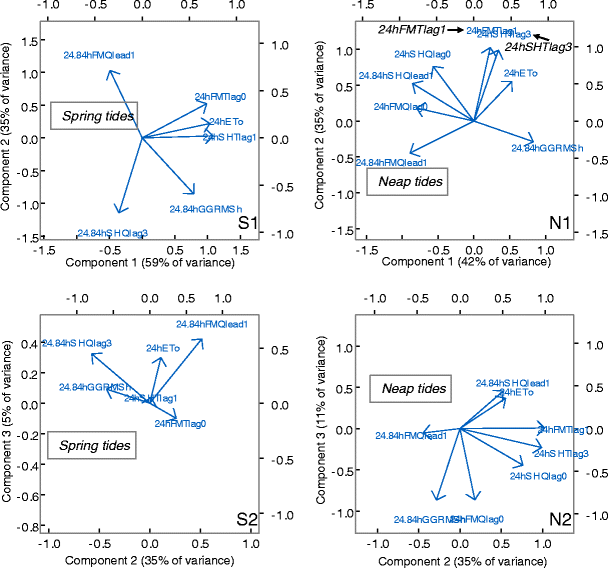
Principal components of driver and lead/lag response relationships. Response leads or lags are maximums from correlation analysis in Fig. 9 (orange circles). The first three components are represented along with variance explained. Left hand column is spring tides; right hand column is neap tides. When correlated with GGRMSh, all data is 24.84-h average of tidally filtered data (n = 94 tidal days from May 1). The corresponding lags are 24.84 h “tidal” days. When correlated with ETo, all data is 24-h average of 15-min data (n = 94 days from May 1) and lags are 24 h days. Response variables are identified by the averaging period (24.84 h or 24 h), the two-letter location abbreviation (“FM” or “SH”) appended to a response descriptor, Q for flow, T for temperature, and the lead or lag value. For example, the maximum correlation between GGRMSh and FM residual flow during spring tides occurs 1 day before the maximum RMS tide height, or “24.84hFMQlead1”

While Fig. 9 attempts to sort out the independent influences of tide strength and meteorology on slough residual flow and water temperature, covariation interactions remain. In particular, Fig. 9 only hints at the residual flow and temperature response to shifting combinations of driver states. For example, we might expect the combination of weak tides and high ETo to drive flows and temperatures differently than weak tides and lower ETo. Similarly we would expect the combination of strong tides and high versus low ETo would drive differential responses, especially at FM where morphology allows more driver interaction. We attempted to partition the data into these four driver permutations but the analysis produced limited insight apparently because the drivers themselves co-vary somewhat. While the drivers are fundamentally independent, ETo is a proxy for meteorological processes that can influence tide heights through wind set-up and fetch orientation as well as atmospheric pressure and ocean temperature anomaly. Finally, the correlation analysis tells us little about the shifting relative influence of the drivers during spring and neap tides.
We submitted the drivers and maximum lead or lag residual flow and temperature response from Fig. 9 (delineated by circles) to a principle components analysis for insight into their variance explanatory power. An exception is the day-average water temperature–ETo correlation during neap tides (Fig. 9, N7 and N8). Water temperature displays a multiple day “memory” of ETo due to the combination of longer neap tide residence time, the heat capacity of water, and the tendency for ETo to be autocorrelated over several days. We submitted to PCA the local peak correlation lags nearest to lag 0 to maintain a reasonable number of observations (realizations are lost as lags match up missing data with observations that must then be dropped). To the PCA, we chose to submit the lag 1 FM temperature–ETo, and lag 3 SH temperature–ETo correlations. We found that results are insensitive to perturbations around this choice. Figure 10 broadly verifies the pair-wise correlations in Fig. 9 with some key clarifications.
Figure 10 demonstrates that both GGRMSh and ETo influence residual temperature and flow outcomes. Moreover, the interactions of driver effects, mediated by morphology, differentiate the slough responses. Depending on spring or neap tide status, one driver can dominate or both can share influence only to shift as the spring-neap tidal harmonic oscillates. Note that the drivers (ETo and GGRMSh) are not correlated so the PCA enforces a nearly orthogonal ordination between them. This somewhat confounds the graphical representation of flow and temperature response components that are influenced by both drivers. We include the third component axis to help untangle this ambiguity. We consider spring and neap tide categories in turn.
Spring Tide Residual Flow
On spring tides, FM residual flow is dominated by tide strength (Fig. 10, S1) with only weak influence by ETo primarily along the component 3 axis (which explains only 5 % of the variance) (Fig. 10, S2). In contrast, ∼3-day lag SH residual flow is driven about equally by ETo and GGRMSh on spring tides (Fig. 10, S1) while components 2 and 3 emphasize the influence of GGRMSh primarily along the component 2 axis (Fig. 10, S2).
Neap Tide Residual Flow
On neap tides, SH residual flow (at both lag-0 day and lead-1 tidal day) is dominated by tide strength with ordination primarily along the component 1 axis (42 % of variance) (Fig. 10, N1). ETo influence on lead-1 tidal day SH flow appears on the components 2 and 3 axes though the lag-0 day SH is not swayed by either driver (Fig. 10, N2). In contrast, lead-1 tidal day and lag-0 day FM residual flow is influenced about equally by ETo and GGRMSh (Fig. 10, N1).
Spring Tide Residual Temperature
Spring tide residual temperature at both sloughs is dominated by meteorological forcing as represented by ETo (Fig. 10, S1–N1). The component 2 and 3 axes demonstrate considerable additional influence of GGRMSh on FM temperature, likely by the interaction of morphology and spring tide heights (Fig. 10, S2).
Neap Tide Residual Temperature
On neap tides, residual temperature at both sloughs is dominated about equally by ETo (Fig. 10, N1). Reduced tidal range and less energetic tidal flow dynamics equalize the driver influence on the otherwise disparate slough morphologies. A summary of driver influences and geomorphic interactions on residual flow and temperature outcomes is presented in Table 3.
Discussion
We contrast a natural and a modified tidal slough to compare the effect of slough geomorphology and hydroperiod on tidal and residual water temperature and flow. At any given time, slough water temperature and flow is influenced by the interacting and shifting influence of sun (as meteorology and tide) and moon (tide). Marsh morphology mediates these dynamics on timescales from hours to centuries via the influence of hydroperiod. The effect of morphology is particularly evident in the natural slough where lunar phase and diel timing of tidal extremes strongly influences tidal and residual flow and temperature. Comparing sloughs, we show that the natural slough is primarily driven by tidal dynamics and meteorology with substantial mediation by characteristic slough morphology. In contrast, the modified slough is influenced by tide and meteorology but there is far less interaction between drivers. This uncoupling of driver interaction is due to the substantial disconnection of slough water from the marsh plain by levees thereby diminishing the hydromorphological linkage between tide and meteorology. Thus, while the sloughs have essentially identical tide and sun influence, the emergent flow and temperature dynamics are different in possibly ecologically significant ways. We note in particular the possible modification of water quality characteristics in water that remains on the tidal marsh plain between overbank tides at FM. Water reaching the marsh plain on spring tides remains ponded or shallowly infiltrated through successive days and hosts biological activity throughout the period. One of the authors routinely observed amphipods and other aquatic invertebrates using ponded marsh plain habitat during the intertidal period between spring tides in marshes throughout the San Francisco Bay region (Culberson et al. 2004). We speculate that primary productivity is enhanced where a slough network includes fortnightly overbank tides as part of its underlying hydraulic character and see evidence of chlorophyll a subsidy from this water as it drains back to the tidal slough network on the subsequent spring sequence (Enright et al., unpublished data). This aspect has not been explored conclusively in this report, but is the subject of future analysis.
At the subtidal timescale, residual flow is driven by superposition of three interacting processes. First, tidal flow asymmetries emerge from interaction between slough morphology and semi-diurnal tide dynamics. Second, residual flows track the fortnightly estuarine fill-and-drain cycle at the lunar timescale. Third, residual flow is forced by diel-to-seasonal evaporation and evapotranspiration within the slough drainage. In parallel, residual water temperature is driven by heat flux from solar insolation, climate factors (wind and humidity), and hydroperiod mediated by morphology. Our analysis attempts to untangle the relative contribution of these influences to slough flow and temperature. We also investigated possible lagged flow and temperature responses, both positive (lag) and negative (lead). We hypothesize that observed differences in flow and temperature response between natural and modified sloughs is ultimately due to how morphology mediates tide, meteorology, and climate drivers.
Untangling Influences and Interactions
We attempted to understand the suite of shifting and interacting driver influences on slough temperature and currents. Our approach was to choose among candidate meteorology and tide driver proxies with PCA, then calculate non-parametric response correlations over a range of leads and lags on data divided into spring and neap tide categories (Fig. 9). Best leads or lags were submitted again to PCA to resolve relative driver influences (Fig. 10). Tides and diel meteorological forcing are closely phased in a ∼29-day precession of moon-sun interaction permutations. Concurrently, semi-diurnal tidal extremes generate shifting degrees of water exchange with the downstream distributary channel. The influence of solar insolation on water temperature depends partly on the residence time of water in the slough which in turn depends on slough length and tidal excursion as a function of position along the slough. Notwithstanding mixing, a given segment of water could reside within a slough for hours or weeks depending on tide strength. During neap tides, multiple along-slough water temperature peaks, caused by tidal trapping, can be superimposed on the 24-h temperature pattern when heated water segments are advected briefly out of the slough only to return on the next flood tide relatively unmixed with the distributary channel (Fig. 4). In the low-order creeks of the natural slough, spring tides drive complete water exchange. During the transition from high–high to low–low tide, even the highest order slough exchanges most of its volume. During lunar maxima, this transition occurs during early morning hours in the summer in recent decades. Much of the high–high tide water is held in overbank shallow storage at night where its temperature is more sensitive to meteorological influence. We have not explored the effect of this process on marsh plain productivity (e.g., as chlorophyll a concentrations or as density of aquatic and terrestrial invertebrates) but we suspect a local primary production export subsidy could occur as a result of shallow overbank retention and slow release (Enright et al., unpublished material). The dynamics of this process will likely change as the diel timing of marsh plain inundation by extreme tides slowly shifts within the 335-year cycle.
Additional confounding influences factor in. While RMS tide strength is a smooth process, overbank flow on the natural slough is a threshold event that step-changes the tidal and residual flow and temperature pattern. We partitioned tidal strength by coarsely dividing the continuum RMS tide height data into spring and neap categories. Each of these factors presents a challenge for untying driver influences and ecological implications.
Leads and Lags
Figure 4 shows how FM flow leads the maximum RMS tide because flood dominant currents appear as soon as the waxing tide exceeds natural bank heights—generally 1–3 days ahead of the lunar maximum. By the time tide heights peak during the lunar maxima, the marsh plain has been flooded and drained possibly multiple times filling low depressions and the field capacity of the soil. Similarly, because we monitored temperature at the slough mouths, observations integrate several processes that impart a lag in the temperature response due to the heat capacity of water, the timing of sun and tides, hydrogeomorphic storage, and transport time to the sensors. Under both spring and neap tide conditions, water temperature lags ETo by 1–2 days. The temperature response mixes out quickly during spring tides but persists for several days during neap tides.
Feedbacks and Thresholds in High-Frequency Flow and Temperature Response
The distribution of tidal currents is different between the sloughs despite equal forcing by tides and meteorology. The maximum flood tide velocity of FM currents is near −0.4 ms−1 while the ebb tide duration is slightly longer and current maximums are no greater than 0.24 ms−1. This asymmetry tends to transport sediment upstream and indeed is a key process that sustains natural tidal marsh elevations in the face of sea-level rise (e.g., Temmerman et al. 2005). Maximum SH ebb and flood currents are nearly equal at approximately ±0.3 ms−1. This difference in ebb-flood current dominance likely accounts for the higher percentage of tidal prism-to-slough volume at FM compared to SH. Flood dominance on natural sloughs is a hydrogeomorphic process feedback that at once transports sediment overbank on high tides, decants it near the channel edge, and builds the very geomorphic threshold that causes flood dominance. As Fig. 5 shows, high-frequency flow–depth and flow–temperature relationships between sloughs are similar most of the time. Only when tide height exceeds natural bank-full height do step-changes in residual flow and temperature responses appear. Compared to the modified slough, the natural slough experiences a fortnight threshold disturbance with consequences for subtidal timescale heat transfer and water flux.
Residual Flow and Temperature Response
At the tidal timescale, flows are primarily driven by tides while temperature is primarily driven by solar insolation. Tidal and diel residuals reveal more complex driver interactions. In the natural slough (FM), residual flow and temperature is driven by interaction between diel tide timing, tide height, degree of water exchange each tide, and slough morphology. The response is complex because factors interact through feedbacks (residual currents affect water exchange, which affects evaporation, which affects residual currents), thresholds (tide height and currents step-change at bank-full height), non-linearity (temperature dynamics), and phasing harmonics (tide and solar maxima precess about 12 °C/day). The modified slough response is less complex. Residual flow at SH responds weakly to tide strength in concert with the greater estuary pattern because levees prevent overbank threshold hydroperiod responses. Evaporation can drive upstream residual currents during neap tides when air temperature, residence time, and water temperature is high. During neap tides, the temperature response is similar between sloughs when morphology differences are minimized.
Sensitivity to Comparison Timescales
We also found that the temporal scale used to compare sloughs reveals differences in morphology (Table 1). Comparing sloughs at the diel timescale, temperature averages and CDF’s are not significantly different regardless of fortnight tide status. When the averaging period is only 3 % longer (nominally 24 h versus 24.84 h), all water temperature and flow means and CDF’s become significantly different. Tidal forcing, as mediated by geomorphology, dominates residual flow and temperature at the tidal time scale on the natural slough (FM). The modified slough (SH) is disconnected from its marsh plain precluding the combined effect of tide strength and meteorology to produce flow and temperature variability.
Temperature Regulation in the Estuary
A key finding of this study is that both sloughs were overall heat sinks during the study period. The average heat flux at FM is −5.8 C m3/s; the average heat flux at SH is −4.8 C m3/s (Fig. 8). FM exhibits tight coupling with the lunar status and tide strength. Temperature outwelling occurs regularly on neap tides when average water elevation in the estuary declines. Spring tide temperature flux at FM responds strongly to tide strength. Full moon RMS tide strength increases into July when the strongest tides occur and overbank flow and storage is greatest. As described above, high summer tides flood the marsh plain in the late evening allowing latent, sensible, and long-wave heat transfer to the atmosphere from water shallowly stored through the night when conditions are cool and often windy. Figure 8 illustrates this process as tidally averaged heat flux but the primary drivers are the interaction of high-frequency tide timing with meteorological factors and slough morphology. Advection is the dominant heat flux transport process at FM during both spring and neap tides though the mechanisms differ. Spring tides allow water levels to exceed bank-full height when channel conveyance suddenly expands and accommodates large advective water and heat fluxes upstream. Neap tide downstream advection at FM is the superposition of diminishing mean estuary water level and the release of water from marsh plain storage by overland, tidal creek, and hyporheic flows. Heat flux at SH is more irregular. The peak neap tide usually fluxes heat downstream for about 2 days unless it coincides with high ETo when evaporation and evapotranspiration can drive residual flow upstream in opposition to estuarine drainage (e.g., compare Fig. 3 and Fig. 8 ∼April 27).
Pulsed Inwelling and Outwelling
The estuarine outwelling hypothesis (focused primarily on detritus and phytoplankton) has been debated since it emerged from classic papers by Teal (1962) and Odum (1968). Nixon (1980) notably questioned the generality of the hypothesis and Odum (2002) suggests that outwelling is better characterized as a pulse phenomenon driven primarily by tides. Our study demonstrates that tidal sloughs both outwell and inwell temperature at tidal and lunar timescales. During neap tides the natural and modified sloughs regularly outwell heat though the modified slough can “inwell” heat if ETo is high and advection by evaporation and evapotranspiration overcomes residual slough outflows. The natural slough (FM) exhibits strong water influx over 8–9 days around the full moon spring tide while accumulation is nearly flat for the intervening three weeks (Fig. 3). When tides overtop slough banks, Fig. 8 shows that FM strongly absorbs heat from the near region. The modified slough (SH) generally imports temperature in a more muted and irregular pattern unless ETo is low on neap tides. Overall, both sloughs are temperature sinks (inwell) with the natural slough more efficiently importing heat. This pattern would likely change if high spring tides occurred during day rather than night as they will 16 decades hence.
Broad Timescale Temperature Dependence
A novel finding of this study is that tidal and residual slough temperature transport depends on the diel and seasonal timing of high spring tides. As discussed above, there is a 335-year cycle in the diel and seasonal timing of semi-diurnal high tides which precesses slightly more than one day per year (Malamud-Roam 2000). In recent and coming decades, high summer spring tides in Suisun Marsh occur in the late evening to early morning hours allowing natural sloughs to store water shallowly on broad marsh plains when the atmosphere is cooler than the water temperature. This is therefore a tidal timescale outcome that depends profoundly on a century-scale astronomical process. Several drivers and processes at intermediate timescales also intervene. Figure 11 shows a conceptual model of natural tidal slough water temperature dependence on interacting driver and process timescales. The purpose of the chart is to illustrate the breadth of timescale variability among interacting processes that influence tidal-to-seasonal timescale slough water temperature. Temperature variability reflects a complex superposition of tide, weather, and climate driver frequencies mediated by morphology. The conceptual model shows how tidal marsh slough flow and temperature is ultimately a complex emergent phenomena forced by unrelated drivers and intermediate outcomes at disparate timescales.

Conceptual model of natural tidal slough water temperature dependence on interacting driver and process timescales. Box width indicates breadth of timescale variability. Ultimate slough water temperature outcome shown in gray
Ecological Implications
Diel timing of extreme tides has implications for ecological processes. Suisun Marsh currently experiences high spring tides near midnight in the summer, and near noon in winter. Over the next 167 years, this pattern will switch. For now, mudflats are dewatered during summer days with implications for biochemical process rates, soil community metabolism, and availability of organisms to shorebirds. Tidal marshes today are inundated during the day in winter—perhaps somewhat before nekton early life stages can fully access and utilize primary-secondary production. High marsh plain production in the late spring and summer is out-welled on maximum ebb tide currents at night making it less available to visual foragers (Simenstad et al. 2000). Three to five decades hence, daytime high tides will occur in late winter and early spring when nekton access and utilization may be improved. Other tidal marsh functions may also slowly shift through the 335-year cycle. For example, within their capacity, nekton accommodates salinity, temperature, forage, and refuge changes within the compressed spatial gradients of tidal marshes. Adaptations to periodic physical processes like the regular availability of cold water at predictable times could be used to competitive advantage and may constitute a selection driver. In addition, the timing of the tidal currents relative to the photo period also has implications for long-term trends deduced from monitoring program data. For example, inferences regarding organisms whose behavior is affected by photo period but whose transport and position in the estuary are affected by the tidal currents may be biased unless the timing between day/night and the tidal cycle is taken into account (Lucas et al. 2006; Burau and Bennett, in prep). Lastly, longer-term tidal processes and the importance of long-residence water deposited on the high marsh in ponds or in near-surface soil horizons have yet to be fully described. Given that most estuary tidal marsh plains hydrogeomorphically regulate bank heights to mean high tide elevations where the higher spring tides flow over bank, we propose this is a critical feature of geomorphic–biologic linkages that makes tidal landscapes so important in the ecology of the estuary at large. Large-scale loss of these landscapes has been correlated with general declines of estuarine species, but few formal causal mechanisms of the sort discussed here have been demonstrated. We think it likely that the spring tide shallow water storage on natural marsh plains would host enhanced primary and secondary production during the “inter-spring” tide sequence. As this “aged” water drains back into high order sloughs following its residence on the marsh plain, the algal and invertebrate species it contains can be transported to and subsidize heterotrophic habitats in the broader estuary (e.g. Cloern 2007). Should this indeed be the case, it is a simple matter to understand how recovering geomorphic patterns to historic proportions might be a desired outcome of tidal marsh restoration in estuaries.
Summary Conclusions
We observed neighboring tidal sloughs with contrasting morphologies and therefore contrasting water surface exposure to solar insolation and heat exchange processes. The natural tidal marsh has elevation discontinuities which produce tidal flow asymmetries and step-changes in hydroperiod. In turn, these intermediate drivers intermittently increase water exposure to air temperature and solar insolation. Meteorological exposure in natural marshes is modulated by phasing of tidal dynamics at hourly, lunar, seasonal, and decadal, and centennial timescales.
-
The natural slough (FM) exhibits comparatively strong flood dominant tidal currents on spring tides due to geomorphic controls. This process likely encourages sediment accretion and vegetation feedbacks thereby strengthening geomorphic control. The modified slough (SH) is ebb dominant similar to the greater estuary pattern. During the warm season, residual flow in the modified slough is driven constantly by meteorology, while residual flow in the natural slough oscillates between meteorological control during neap tides and morphology-tide interaction control during spring tides.
-
At the tidal timescale, flows are strongly driven by tidal harmonic forcing while slough temperatures in the sloughs are driven by daily solar insolation and meteorological conditions. For subtidal timescales (greater than ∼1 day), slough flows and temperatures are driven by complex and shifting interactions between heat transfer mechanisms and tide-morphology interactions.
-
Both sloughs exhibit overall negative (upstream directed) water flux in warm months due to evaporation and transpiration, though the interaction mechanisms and pattern differ. In turn, both sloughs are net temperature sinks primarily by advective transport with residual water flow. FM temperature advection and dispersion are coherent with lunar cycle tidal forcing and its morphology linkage to evaporation and transpiration. SH temperature advection is irregular and lower magnitude.
-
Because we monitored temperature and flow at the slough mouths, measurements integrate several processes that lead or lag the temporal pattern of driver energy. FM residual flow leads the maximum RMS tide because flood dominant currents appear as soon as waxing tides exceed the natural bank height—generally 1–3 days ahead of the lunar maximum. Residual temperature response generally lags drivers due to the heat capacity of water, geomorphic storage, transport time to the sensors, and the status of the 335-year precession of the diel timing of extreme tides.
-
Phasing of a 335-year precession of diel timing of tidal extremes exerts a profound tidal and fortnight cooling effect on both sloughs and the estuary at large. Morphological mediation intensifies the effect on the natural slough.
-
Driver interactions in the modified slough are uncoupled by the complete disconnection of slough water from the former marsh plain by levees.
-
Tidal slough residual flow and temperature are an emergent response of a cascade of processes that are mediated by morphology. Untangling driver influences is not straightforward. The drivers we used can act together to influence residual flow or temperature, or they can act in opposite directions with the outcome reflecting subtle changes in relative strength of each driver.
-
High-frequency water temperature regulation appears to be a key function of natural tidal sloughs and depends critically on geomorphic mediation. Natural tidal marsh morphology links tidal forcing to broad timescale water temperature control. This work demonstrates how high-frequency current and water temperature variability emerges from multiple timescale interactions between tidal harmonics, tidal marsh morphology, and solar insolation.
-
We see no reason to believe that these finding should not broadly hold for tidal marshes in other estuaries. The cooling function of natural tidal sloughs is an important ecosystem service and a likely species selection driver. Tidal marsh restoration efforts that return historical current and temperature patterns may improve competitive advantage and resilience of native species in the face of contemporary estuarine system stressors.
The levees of the modified slough disconnect not only water from land, but also water from atmospheric interaction. The severed land–water interactions profoundly change current and water temperature dynamics. The northern reach of the San Francisco estuary contains hundreds of modified or disconnected terminal tidal sloughs where the current and temperature regime is probably considerably changed. A proper characterization of the change would require sophisticated modeling. In contrast, historical tidal marshes were driven by interaction of meteorology, tide, and river inputs and shaped by sedimentation—vegetation feedbacks. The key linking process is hydroperiod mediation by morphology.
Based on our results, we speculate that pre-development currents and temperature regimes in the San Francisco Estuary were significantly influenced by tidal hydroperiod interaction with natural tidal marsh morphology. Strong temperature gradients and periodic low temperature refugia would be produced in a regular pattern in tidal marsh creeks. Native species may have evolved adaptations to the pattern. The 335-year cycle of diel tidal extreme timing assures that shallow hydroperiod dynamics on tidal marsh plains will coincide with mid-day solar insolation in the next century which will likely produce higher temperatures. Other estuarine components like mudflats are also sensitive to the diel high tide timing cycle. Today, mudflats are generally more exposed to solar insolation in summer with consequences for a cascade of outcomes like soil metabolism and wading bird foraging. These outcomes may express very differently the next century.
References
Allen, R.G., J.H. Prueger, and R.W. Hill. 1992. Evapotranspiration from isolated stands of hydrophytes: cattail and bulrush. Transactions of ASAE 35(4): 1191–1198.
Atwater, B.F., S.G. Conard, J.N. Dowden, C.W. Hedel, R.L. MacDonald, W. Savage. 1979. History, landforms, and vegetation of the estuary’s tidal marshes. In: San Francisco Bay: the urbanized Estuary; T.J. Conomos (ed.). American Association for the Advancement of Science; pp 347-386.
Aubrey, D.G., and P.E. Speer. 1985. A study of non-linear tidal propagation in shallow inlet/estuarine systems, part I: observations. Estuarine, Coastal and Shelf Science 21: 185–205.
Cartwright, DE. 1999. Tides, a scientific history. Cambridge University Press.
Cloern, J.E. 2007. Habitat connectivity and ecosystem productivity: implications from a simple model. The American Naturalist 169.
Crabtree, S.J., and B. Kjerfve. 1977. The radiation balance over a salt marsh. Boundary Layer Meteorology 14(1978): 59–66.
Culberson, S.D., T.C. Foin, and J.N. Collins. 2004. The role of sedimentation in estuarine marsh development within the San Francisco Estuary, California, USA. Journal of Coastal Research 20: 970–979.
DiLorenzo, J.L. 1988. The overtide and filtering response of small inlet/bay systems. In Hydrodynamics and sediment dynamics of tidal inlets, eds. D. G. Aubrey and L. Weishar, 24–53. New York, NY: Springer.
Dronkers, J. 1986. Tidal asymmetry and estuarine morphology. Netherlands Journal of Sea Research 20(2): 117–131.
DWR 2011. California Irrigation Management Information System (CIMIS) data. California Department of Water Resources. http://wwwcimis.water.ca.gov/cimis/data.jsp
Dyer, K.R. 1973. Estuaries: a physical introduction. Wiley. 210 pp.
Fischer, H.B., J.E. List, C.R. Koh, J. Imberger and N.H. Brooks. 1979. Mixing in inland and coastal waterways. Academic.
Friedrichs, C.T., and D.G. Aubrey. 1988. Tidal distortion in shallow well-mixed estuaries: a synthesis. Estuarine, Coastal and Shelf Science, v. 27: 521–545.
Friedrichs, C.T., and J.E. Perry. 2001. Tidal salt marsh morphodynamics: a synthesis. Journal of Coastal Research 27: 7–37.
French, J.R., and D.R. Stoddart. 1992. Hydrodynamics of salt marsh creek systems: implication for marsh morphological development and material exchange. Earth Surface Processes and Landforms 17: 235–252.
Godin, G. 1972. The analysis of tides. University of Toronto Press
Hardisty, J. Estuaries: monitoring and modeling the physical system. Blackwell; Malden, MA. 157 pp.
Harrison, S.J., and A.P. Phizacklea. 1987. Vertical temperature gradients in muddy intertidal settlements in the Forth Estuary, Scotland. Limnology and Oceanography 32(4): 954–963.
Holland, A.F., D.M. Sanger, C.P. Gawle, S.B. Lerberg, M.S. Santiago, G.M.H. Riekerk, L.E. Zimmerman, and G.I. Scott. 2004. Linkages between tidal creek ecosystems and the landscape and demographic attributes of their watersheds. Journal of Experimental Marine Biology and Ecology 298: 151–178.
Kirwan, M.L., and A.B. Murray, 2007. A coupled geomorphic and ecological model of tidal marsh evolution. Proceedings of the National Academy of Sciences 104(15): 6118–6122.
Kneib, R.T. 1997. The role of tidal marshes in the ecology of estuarine nekton. Oceanography and Marine Biology: an Annual Review 35: 163–220.
Kneib, R., C. Simenstad, M. Nobriga, and D. Talley. 2008. Tidal marsh conceptual model. Sacramento (CA): Delta Regional Ecosystem Restoration Implementation Plan.
Lawrence, D.S.L., J.R.L. Allen, and G.M. Havelock. 2004. Saltmarsh morphodynamics: an investigation of tidal flows and marsh channel equilibrium. Journal of Coastal Research 20(1): 301–316.
Lucas, L.V., D.M. Sereno, J.R. Burau, T.S. Shraga, C.B. Lopez, M.T. Stacey, K.V. Parchevshy, and V.P. Parchevshy. 2006. Intradaily variability of water quality in a shallow tidal lagoon: mechanisms and implications. Estuaries and Coasts 29(5): 711–730.
Malamud-Roam, K.P. 2000. Tidal Regimes and tide marsh hydroperiod in the San Francisco Estuary: Theory and implications for ecological restoration. Dissertation, University of California, Berkeley.
McKay, P., and D. DiIorio. 2008. Heat budget for a shallow, sinuous salt marsh estuary. Continental Shelf Research 28: 1740–1753.
McLusky, D.S., and M. Elliott. 2004. The estuarine ecosystem, ecology, threats and management. Third edition. Oxford University Press.
Mitsch, W.J., and J.G. Gosslink. 2007. Wetlands--4th ed. John Wiley & Sons.
Monroe, M., P.R. Olofson , J.N. Collins, R.M. Grossinger, J. Haltiner, and C. Wilcox. 1999. Baylands ecosystem habitat goals; San Francisco Bay Area Wetlands Ecosystem Goals Project. U.S. Environmental Protection Agency, San Francisco, Calif./S.F. Bay Regional Water Quality Control Board, Oakland, Calif.
Moyle, P.B., W.A. Bennett, W.E. Fleenor, and J.R. Lund. 2010. Habitat variability and complexity in the upper San Francisco Estuary. San Francisco Estuary and Watershed Science, 8(3).
Myrick, R.M., and L.B. Leopold. 1963. Hydraulic geometry of a small tidal estuary, physiographic and hydraulic studies of rivers, U.S. Geological Survey Professional Paper 422-B, 18p
Nixon, S.W. 1980. Between coastal marshes and coastal waters--a review of twenty years of speculation and research on the role of salt marshes in estuarine productivity and water chemistry, p. 437-525. In, R. Hamilton and K.B. MacDonald [ed.] Estuarine and wetlands processes. Plenum Press, New York, NY.
Odum, E.P. 1968. Energy flow in ecosystems: A historical review. Amer. Zool. 8(1): 11–18.
Odum, E.P. 2002. Tidal marshes as outwelling/pulsing systems. In, M. Weinstein and D.A. Kreeger [ed.] Concepts and controversies in tidal marsh ecology, pp 3-7. Springe, Netherlands.
Parker, B. 2011. The tide predictions for D-Day. Physics Today 64(9): 35–40.
Pethick, J.S. 1980. Velocity surges and asymmetry in tidal channels. Estuarine and Coastal Marine Science 11: 331–345.
Portnoy, J.W., and A.E. Giblin. 1997. Effects of historic tidal restrictions on salt marsh sediment chemistry. Biogeochemistry 36: 275–303.
Rattray, M., and J.G. Dworski. 1980. Comparison of methods for analysis of the transverse and vertical circulation contributions to the longitudinal advective salt flux in estuaries. Estuarine Coastal Mar. Sci. 11: 515–536.
Reed, D.J. 1988. Sediment dynamics and deposition in a retreating coastal salt marsh. Estuarine, Coastal and Shelf Science 26: 67–79.
Silvestri S., and M. Marani. 2004. Salt-marsh vegetation and morphology: basic physiology, modeling, and remote sensing observations, In Ecogeomorphology of Tidal Marshes, eds. S.
Simenstad, C.A., W.G. Hood, R.M. Thom, D.A. Levy, and D.L. Bottom. 2000. Landscape structure and scale constraints on restoring estuarine wetlands for Pacific Coast juvenile fishes. In Concepts and controversies in tidal marsh ecology, ed. M.P. Weinstein and D.A. Kreeger, pp. 597–630. Dordrecht, Netherlands: Kluwer.
Stacey, M.T, and S.G. Monismith. 2008. Temperature dynamics of the Sacramento–San Joaquin Delta. Unpublished conceptual model compiled for the CALFED ERP Program DRERIP program element (website here: http://www.dfg.ca.gov/ERP/conceptual_models.asp)
Teal, J.M. 1962. Energy flow in the salt marsh ecosystem of Georgia. Ecology 43: 614–624.
Temmerman, S., T.J. Bouma, G. Grovers, and D. Lauwaet. 2005. Flow paths of water and sediment in a tidal marsh: relation with marsh developmental stage and tidal inundation height. Estuaries 28(3): 338–352.
Turner, R.E. 2004. Coastal wetland subsidence arising from local hydrologic manipulations. Estuaries 27(2): 265–272.
Vileisis, A. 1999. Discovering the unknown landscape: a history of America’s wetlands. Washington DC: Island.
Walton, T.L. 2002. Tidal velocity asymmetry at inlets. ERDC/CHL CHETN IV-47. U.S. Army Engineer Research and Development Center, Vicksburg, MS Thesis, http://chl.erdc.usace.army.mil
Walters, R.A., R.T. Cheng, and T.J. Conomos. 1982. Time scales of circulation and mixing processes of San Francisco Bay waters. Hydrobiologia 129: I3–36.
Walters, R.A., and J.W. Gartner. 1985. Subtidal sea level and current variations in the northern reach of San Francisco Bay. Estuarine, Coastal and Shelf Science 21: 7–32.
Warner, J., D.H. Schoellhamer, J.R. Burau, and G. Schladow. 2002. Effects of tidal current phase at the junction of two straits. Continental Shelf Research 22(11): 1629–1642.
Wheaton, F.W. 1977. Aquacultural engineering, 708 pp. New York: Wiley.
Wiens, J.A. 2002. Riverine landscapes: taking landscape ecology into the water. FreshwaterBiology 47: 501–515.
Acknowledgments
Thanks to two anonymous reviewers for comments that improved the paper. One reviewer in particular exemplified the spirit of scientific peer review by offering an extremely careful and thoughtful appraisal which greatly clarified the manuscript. We are humbled and honored by the depth of consideration. Thanks to Curt Battenfeld, Angelo Garcia and Randy Smith for capable field assistance. Thanks to the Interagency Ecological Program for bridge funding.
Author information
Authors and Affiliations
Corresponding author
Rights and permissions
Open Access This article is distributed under the terms of the Creative Commons Attribution License which permits any use, distribution, and reproduction in any medium, provided the original author(s) and the source are credited.
About this article
Cite this article
Enright, C., Culberson, S.D. & Burau, J.R. Broad Timescale Forcing and Geomorphic Mediation of Tidal Marsh Flow and Temperature Dynamics. Estuaries and Coasts 36, 1319–1339 (2013). https://doi.org/10.1007/s12237-013-9639-7
Received:
Revised:
Accepted:
Published:
Issue Date:
DOI: https://doi.org/10.1007/s12237-013-9639-7