Adaptive Kuwahara filter

Abstract

A new filter was created by improving the standard Kuwahara filter. It allows more efficient noise reduction without blurring the edges and image preparation for segmentation and further analyses operations. One of the biggest and most common restrictions encountered in filter algorithms is the need for a declarative definition of the filter window size or the number of iterations that an operation should be repeated. In the case of the proposed solution, we are dealing with automatic adaptation of the algorithm to the local environment of each pixel in the processed image.

Introduction

Contextual transformations are operations in which the outcome depends on a modified pixel and its surroundings [4, 5]. Alternatively, the name “digital filters” is also used. The application of digital filters is very wide, and they are used in many areas of life including radiology, automatic control systems and machine vision. The main applications of digital filters are as follows:

• suppressing unwanted noise,

• improving image sharpness,

• removing specific defects ,

• visualizing certain image features,

• reconstructing partly destroyed images.

In this paper, I address the issues of reducing noise from digital images and present a new highly efficient algorithm. The issue of noise or other errors is extremely important because they can appear during image acquisition, transmission or compression and decompression. Therefore, image filtering is a very important aspect of image processing and preparation for further work such as image compression, edge detection or image segmentation. The application of noise reduction algorithms is also extensively used in medical imaging. A large number of articles discussing this subject have been published, e.g., [2, 3].

However, at the beginning I would like to present the presentation of the standard commonly used algorithms and to clarify the terms used.

It is highly likely that there exist filters that remove noise from digital images faster, gain a better rate of bug fixing or modify the edges of objects less than those used in this study. However, a comparison of all the existing solutions would require a large and difficult to estimate amount of work, at least because of the need to provide a similar level of implementation and other conditions of the experiment, and thus, it would exceed significantly the planned scope of the study. There is nothing, however, to prevent extending the scope of the comparison and to present its results in future publications.

The general concept of the context filters is to create the output image on the basis of the source image in such a way that the value of each pixel at coordinates (x,y) in the output image is determined based on a certain neighborhood of the pixel at coordinates (x,y) in the source image [4–9]. This neighborhood is defined as a filter window. Usually, it is assumed that the filter window is square and the size (width and height) is an odd integer number, e.g., $3\times 3, 5\times 5, 7\times 7$. In this case, a pixel at coordinates (x,y) is exactly in the middle of the filter window. There are also solutions that collect statistical information about the entire image and then use them during the processing of each pixel.

Context filters

Average filter

The average filter is one of the simplest filters enabling removing noise and distortion. Unfortunately, it also introduces changes in the areas that have originally been noise and distortion free.

Let us assume that we construct a filter operating on the window ${N} \times {N}$. In this case, the resulting value of the pixel is the average value of all the pixels contained within the current analysis window of the source image

$$\begin{aligned} m_{\theta }=\frac{1}{{N} \times {N}} \times \sum \limits _{(x,y) \in \theta } \varphi \big (f(x,y)\big ) \end{aligned}$$

(1)

where:

• f is the source image function,

• f(x,y) is the value of the pixel at coordinates (x, y),

• $\varphi$ is a function calculating the value of a particular pixel. This function can take different values depending on the color space, the format or the depth of the image,

• ${{N} \times {N}}$ is the number of pixels in the current window,

• $\theta$ represents the collection of pixels in the current window.

Some of the largest disadvantages of the average filter are blurring noise and significant modification of correct pixels.

Median filter

The concept of the median filter is very similar to that shown above. The only difference is that all elements in the current filter window have to be sorted and ordered in an ascending sequence. The resulting value is the value of the item in the exact middle point of the ordered sequence (position $\frac{{N} \times {N}}{2}$ for ${N} \times {N}$ window).

With the use of this filter, one can very effectively remove any local noise, without blurring the noise to larger areas, which was a major disadvantage of the average filter.

Adaptive median filter

The adaptive median filter, as its name suggests, is a modification of the median filter. This modification consists in allowing a situation where the window size is not constant, but changes dynamically according to the context. If you select too small a window, the median filter could not handle all the noises, while too large a window results in dissolving the smaller but desired image detail.

The adaptive median filter algorithm has the following form:

Step 1 For each pixel $\textit{f}\,\,(\textit{x},\textit{y})$ of the image f, we determine the list of neighbors in $\textit{N} \times \textit{N}$ window. Among these elements, we calculate the minimum, middle (median) and the maximum value and denote these values as $f_\mathrm{min}$, $f_\mathrm{med}$ and $f_\mathrm{max}$, respectively.

Step 2 If $f_\mathrm{min}=f_\mathrm{med}$ or $f_\mathrm{med}=f_\mathrm{max}$, then the size of filter window is increasing and the actions done in the previous step for the new window have to be repeated. Otherwise, go to the next step.

For obvious reasons, there must exist the maximum allowable window size. If it is not possible to further increase the filter window size, then the output pixel is set to the neighbors list middle value determined in the previous step ($f_\mathrm{med}$).

Step 3 If $f_\mathrm{min}<f(x,y)$ and $f(x,y)<f_\mathrm{max}$, then the output pixel takes the value of f(x, y), which means that item is not modified. Otherwise, the output pixel is set to the neighbors list middle value determined in the first step ($f_\mathrm{med}$).

This filter is able to reduce even a large noise. Unfortunately, the high computational complexity of this filter is quite a serious disadvantage. In addition, if the maximum window size is set to too small a value, we can get unsatisfactory results. However, too large a window size may cause very unsatisfactory execution time.

Kuwahara filter

Because the contour plays a very important role in the process of image analysis [4, 9], it is very important to ensure that the image smoothing does not affect the sharpness of contours. This could cause serious problems later, during segmentation. The Kuwahara filter [1] is an example of a filter which meets these requirements. This filter can be constructed for any window size. For readability, the algorithm will be described for the window of size of $3\times 3$.

The filter window should be divided into four areas. Let us denote them as $\theta _{k}$ where $k\in \{0,1,2,3\}$. These four areas are highlighted in Fig. 1. The center pixel is marked with black color. If a square filter window consists of $(2\times n+1)\times (2\times n+1)$ elements, then each area will contain exactly $(n+1)\times (n+1)$ elements. In the described case, the filter window size is $3\times 3$, so each area will consist of four elements. Then, for each of these areas, the values of average $m_{k}$ and variance $\delta _{k}^{2}$ are calculated. The average and variance are calculated according to the formula:

$$\begin{aligned} m_{k}= & {} \frac{1}{(n+1)\times (n+1)} \times \sum \limits _{(x,y) \in \theta _{k}} \varphi \big (f(x,y)\big ) \end{aligned}$$

(2)

$$\begin{aligned} \delta _{k}^{2}= & {} \frac{1}{(n+1)\times (n+1)} \times \sum \limits _{(x,y) \in \theta _{k}} \Big [ \varphi \big (f(x,y)\big ) - m_{k} \Big ]^2\nonumber \\ \end{aligned}$$

(3)

where:

• $k \in \{0,1,2,3\}$,

  Fig. 1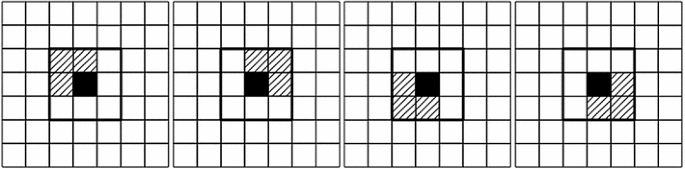

  

  Kuwahara filter window with highlighted four areas $\theta _{k}$

• f is the source image function,

• f(x, y) is the value of the pixel at coordinates (x, y),

• $\varphi$ is a function calculating the value of a particular pixel,

• $\frac{1}{(n+1)\times (n+1)}$ is the number of pixels in the current area,

• n is the value obtained directly from the filter window size.

Finally, we compare the variance of all four areas and look for an index of the area for which the variance is the smallest.

$$\begin{aligned} \delta _\mathrm{min}^{2} = \min _{k \in \{1,2,3,4\}} \big ( \delta _{k}^{2} \big ) \end{aligned}$$

(4)

The resulting value of the center pixel is the average value of the area for which the variance was the smallest.

The result of increasing the size of the filter windows will be better noise reduction, but it can cause blurring of small details in the analyzed image.

Adaptive Kuwahara filter

The adaptive Kuwahara filter algorithm was created by combining two other filters: the adaptive median filter and the Kuwahara filter. The most important feature of the adaptive median filter is the possibility to adjust the window size of the filter to the results of a partial analysis obtained during the operation, whereas the major task of the Kuwahara filter is smoothing colors intensity and removing small noise while maintaining the edges. Unfortunately, neither of these filters are flaw free.

The first blurs the edges, making further analysis even more difficult. Furthermore, in connection with variable window size, computational complexity of the filter can be much higher than of other filters. On the other hand, the Kuwahara filter retains the edges, but it requires a strictly defined window size. An undesirable effect of the second filter is very significant pixelation, which is a mosaic of large, homogeneous, often rectangular areas.

The differences in the operation of the various algorithms can be seen in Figs. 2, 3, 4, 5, 6 and 7. Each figure consists of a sequence of five images; starting from the left side, they represent (a) original image, (b) after applying Kuwahara filter where window size is constant and equals $3\times 3$, (c) after applying Kuwahara filter where window size is constant and equals $11\times 11$, (d) after applying adaptive median filter and (e) after applying adaptive Kuwahara filter.

Fig. 2

Comparison of adaptive Kuwahara filter with other filters. Image without noise. Labels a, b, c, d and e correspond to a original image, b Kuwahara filter with constant window size $3\times 3$, c Kuwahara filter with constant window size $11\times 11$, d adaptive median filter and e adaptive Kuwahara filter

Fig. 3

Comparison of adaptive Kuwahara filter with other filters. Image has been modified by the addition of salt and pepper noise with uniform distribution on the surface of 1 %. Labels a, b, c, d and e correspond to a original image, b Kuwahara filter with constant window size $3\times 3$, c Kuwahara filter with constant window size $11\times 11$, d adaptive median filter and e adaptive Kuwahara filter

Fig. 4

Comparison of adaptive Kuwahara filter with other filters. Image has been modified by the addition of salt and pepper noise with uniform distribution on the surface of 2 %. Labels a, b, c, d and e correspond to a original image, b Kuwahara filter with constant window size $3\times 3$, c Kuwahara filter with constant window size $11\times 11$, d adaptive median filter and e adaptive Kuwahara filter

Fig. 5

Comparison of adaptive Kuwahara filter with other filters. Image has been modified by the addition of additive salt and pepper noise with uniform distribution on the surface of 5 %. Labels a, b, c, d and e correspond to a original image, b Kuwahara filter with constant window size $3\times 3$, c Kuwahara filter with constant window size $11\times 11$, d adaptive median filter and e adaptive Kuwahara filter

Fig. 6

Comparison of adaptive Kuwahara filter with other filters. Image has been modified by the addition of additive salt and pepper noise with uniform distribution on the surface of 25 %. Labels a, b, c, d and e correspond to a original image, b Kuwahara filter with constant window size $3\times 3$, c Kuwahara filter with constant window size $11\times 11$, d adaptive median filter and e adaptive Kuwahara filter

Fig. 7

Comparison of adaptive Kuwahara filter with other filters. Image has been modified by the addition of additive salt and pepper noise with uniform distribution on the surface of 25 % and white grid. Labels a, b, c, d and e correspond to a original image, b Kuwahara filter with constant window size $3\times 3$, c Kuwahara filter with constant window size $11\times 11$, d adaptive median filter and e adaptive Kuwahara filter

In addition, one can see how the presented filters behave in relation to images with different noise levels. Figure 2 is the original image without additional noise. Figure 3 has been modified by the addition of salt and pepper noise with uniform distribution on the surface of 1 %. Figure 4 has been modified by the addition of salt and pepper noise with uniform distribution on the surface of 2 %. Figure 5 has been modified by the addition of additive salt and pepper noise with uniform distribution on the surface of 5 %. The brightness of the randomly selected pixel was changed (increased or decreased) by 25 % of the maximum value. Figure 6, like the previous one, has been modified by the addition of additive salt and pepper noise with uniform distribution on the surface of 25 %. The last picture (Fig. 7) is a modification of the previous one by adding a white grid.

Algorithm description

The standard Kuwahara filter requires a strictly defined window size. In the case of the proposed modification of the filter, the window size is changing, just as it did in the adaptive median filter, depending on the local properties of the image. The initial window size is $3\times 3$.

Step 1 The filter window should be divided into four areas by following the original algorithm. Let us denote them as $\theta _{k}$ where $k \in \{0,1,2,3\}$. Initially, each of these areas will consist of four pixels. For the purposes of this algorithm, let us call these four areas the basic areas.

Step 2 For each of these areas, the values of mean $m_{k}$ and variance $\delta _\mathrm{min}^{2}$ are calculated. As before, the value of a specific pixel can be the value of color intensity, brightness or any other calculated value. The mean and variance are calculated according to the formula:

$$\begin{aligned} m_{k}= & {} \frac{1}{N_{k}} \times \sum \limits _{(x,y) \in \theta _{k}} \varphi \big (f(x,y)\big ) \end{aligned}$$

(5)

$$\begin{aligned} \delta _{k}^{2}= & {} \frac{1}{N_{k}} \times \sum \limits _{(x,y) \in \theta _{k}} \Big [ \varphi \big (f(x,y)\big ) - m_{k} \Big ]^2 \end{aligned}$$

(6)

where:

• $k \in \{0,1,2,3\}$,

• f is the source image function,

• $\varphi$ is a function calculating the value of a particular pixel,

• $N_{k}$ is the number of pixels in the current area, in the first cycle the value is 4.

Step 3 Each of the basic areas is considered separately. For the chosen area, the size of the window is increased by 1. Next, for the new window size, mean $\overline{m_{k}}$ and variance $\overline{\delta _{k}^{2}}$ have to be calculated according to the formulas presented in the previous step.

An example can be seen in Fig. 8. The filter window central element and the elements included in area $\theta _{k}$ as it increases are highlighted.

Fig. 8

Resizing the filter window and items included in the new area $\theta _{k}$

If the variance of the new area ($\overline{\delta _{k}^{2}}$) is smaller than before the resizing of the filter window ($\delta _{k}^{2}$), then the mean and variance of the basic area k take the newly calculated values:

$$\begin{aligned} m_{k}:= & {} \overline{m_{k}} \end{aligned}$$

(7)

$$\begin{aligned} \delta _{k}^{2}:= & {} \overline{\delta _{k}^{2}} \end{aligned}$$

(8)

Then we continue to increase the size of the window for the basic area selected in the current step until its size reaches the maximum allowable size or until the variance of the newly enlarged area is greater than that calculated in the previous cycle of the algorithm. In this way, the minimum variance and the corresponding average value will be achieved for the basic area k. For further calculations, it is not necessary to know the size of the window for which the variance and the mean values were calculated.

The calculations shown in Step 3 must be repeated separately for each of the four basic areas.

Step 4 Finally, we compare the variance of all four areas. At this stage, each of the basic areas can be made with different quantity of items. We are looking for an index of the area for which the variance is the smallest.

$$\begin{aligned} \delta _\mathrm{min}^{2} = \min _{k \in \{1,2,3,4\}} \big ( \delta _{k}^{2} \big ) \end{aligned}$$

(9)

The resulting value of the output pixel is the average value of the basic area for which the variance was the smallest. Figure 9 presents an example of possible window size distribution for items included in the four basic areas and common parts of these areas. The center pixel is marked with black color.

Fig. 9

An example of possible window size distribution for basic areas

Figure 10 presents a block diagram showing the operation of the developed algorithm.

Fig. 10

Block diagram of the adaptive Kuwahara filter

Comparison of algorithms

One of the most serious problems of the edge preserving smoothing filters is causing over blurring and removing details in low-contrast regions. Nonlinear edge preserving smoothing filters have been an actively researched continuously for decades. Worth mentioning is the articles [10–15] where authors present various approaches to the problem of edge preserving smoothing filters.

Very interesting approach of the advanced modification of the Kuwahara filter was introduced in the work [16] where authors used very sophisticated mathematical description on the theoretical considerations. The paper in any way does not cover the technical aspects of implementation or optimization. The only suggestion placed by the authors was information that definite integral can be approximate by discrete sums. It is a trivial remark and in any meaningful way does not clean the complexity of implementation.

The article authors suggest that processing time depends on the size of the filter kernel, the number of sectors and the size of input. However, based on the exemplary, implementation and the description of the algorithm can be concluded that the computational complexity is also influenced by the radius h parameter which is used for mapping $\varOmega$ into a disk of h radius. There were not, however, shown any estimations considering the computational complexity of the presented algorithm. But, on the basis of the theoretical considerations, it can easily be concluded that the computational complexity of the adaptive Kuwahara filter is significantly smaller than anisotropic Kuwahara filter. This is, due to among other things, because the necessity of smoothing with a Gaussian filter and defining elliptic filter kernels. In addition, for each regions, in order to obtain weighted local averages and variances, complex calculations have to be performed.

The separate aspect is the fact that anisotropic Kuwahara filter was primarily designed for preserving shape boundaries and achieving the painterly effect look, without having to deal with individual brush strokes. One of the major similarities of the two filters (adaptive Kuwahara filter and anisotropic Kuwahara filter) is a robust against high-contrast noise, and the difference is the fact that the proposed new approach does not require from the user to provide any additional parameters.

Short tests were conducted to compare the quality of the noise reduction in the analyzed filters. Tests include previously discussed algorithms and anisotropic Kuwahara filter. Original images have been modified by the addition of additive salt and pepper noise with uniform distribution on the surface of 25 %. Finally, the original and filtered were compared with the use of the mean squared error algorithm. The results are shown in Table 1. In the MSE algorithm, smaller value indicates a better result. Figure 11 presents a sequence of seven images; starting from the left side, they represent original image, noised image, after applying average filter with where window size $7\times 7$, after applying adaptive median filter, after applying Kuwahara filter where window size is constant and equals $7\times 7$, after applying adaptive Kuwahara filter and finally after applying anisotropic Kuwahara filter.

Table 1 Comparation of the noise reduction filters (MSE algorithm)

Fig. 11

Comparation of the noise reduction filters on the Lena image

One can easily see proposed algorithm guarantees to achieve very good results. For the all examined examples, the effects of the adaptive Kuwahara filter were better than anisotropic Kuwahara filter. In addition, taking into account, lower computational complexity adaptive Kuwahara filter can be considered as a strong contender of the anisotropic Kuwahara filter.

Summary

On the basis of the examples, it can be easily noticed that the modified Kuwahara filter is a promising improvement. The most important of its features includes the ability to preserving the edges of the objects. After applying the proposed filter, both the objects and the edges are changed much less than when using the standard Kuwahara filter. Additionally, the tendency to pixelation, compared to the standard Kuwahara filter, has been greatly reduced. Furthermore, it has the ability to remove noise from an image with comparable efficacy as that of the adaptive median filter as well as it retains a greater variety of color intensity in relation to the Kuwahara filter what can be confirmed by analyzing the results of MSE algorithm.

While creating presented solution, very important aspect was the optimization of computational complexity. The adaptive Kuwahara filter is very fast in operation, especially compared to the adaptive median filter. This suggests that the direction for further research should be a detailed analysis of the computational complexity of created algorithm and its comparison with other filters.

References

Kuwahara, M., Hachimura, K., Eiho, S., Kinoshita, M.: Processing of RI-angiocardiographic images. In: Preston Jr, K., Onoe, M. (eds.) Digital Processing of Biomedical Images, pp. 187–202. Plenum, New York (1976)
Söderman, M., Holmin, S., Andersson, T., Palmgren, C., Babić, D., Hoornaert, B.: Image noise reduction algorithm for digital subtraction angiography: clinical results. Radiology 269(2), 553–560 (2013)
Leipsic, J., LaBounty, T.M., Heilbron, B., Min, J.K., Mancini, G.B.J., Lin, F.Y., Taylor, C., Dunning, A., Earls, J.P.: Adaptive statistical iterative reconstruction: assessment of image noise and image quality in coronary CT angiography. Cardiopulm. Imaging, 195, September (2010)
Pratt, W.K.: Digital Image Processing. Wiley, New York (2001)
Rosenfeld, A.: Picture Processing by Computer. Academic Press, New York (1969)
Bovik, A.C.: Handbook of Image and Video Processing. Academic Press, New York (2000)
Hall, E.L.: Computer Image Processing and Recognition. Academic Press, New York (1979)
Jahne, B.: Digital Image Processing. Springer, Berlin, Heidelberg (2005)
Sonka, M., Hlavac, V., Boyle, R.: Image Processing Analysis and Machine Vision. Springer, US (1993)
Tomita, F., Tsuji, S.: Extraction of multiple regions by smoothing in selected neighborhoods. IEEE Trans. Syst. Man Cybern. 7, 107–109 (1977)
Nagao, M., Matsuyama, T.: Edge preserving smoothing. Comput. Gr. Image Process. 9, 394–407 (1979)
van den Boomgaard, R.: Decomposition of the Kuwahara-Nagao operator in terms of linear smoothing and mor- phological sharpening. ISMM 2002 (2002)
Hu, H., de Haan, G.: Adding explicit content classification to nonlinear filters. Signal, Image Video Process. 5(3), 291–305 (2011)
Nasimudeen, A., Nair, Madhu S., Tatavarti, Rao: Directional switching median filter using boundary discriminative noise detection by elimination. Signal, Image Video Process. 6(4), 613–624 (2012)
Bhadouria, V.S., Ghoshal, D., Siddiqi, A.H.: A new approach for high density saturated impulse noise removal using decision-based coupled window median filter. Signal, Image Video Process. 8(1), 71–84 (2014)
Kyprianidis, J.E., Kang, H., Döllner, J.: Image and video abstraction by anisotropic Kuwahara filtering. Comput. Gr. Forum, pp. 1955–1963 (2009)
Author information
Authors and Affiliations
Corresponding author
Rights and permissions
Open Access This article is distributed under the terms of the Creative Commons Attribution 4.0 International License (http://creativecommons.org/licenses/by/4.0/), which permits unrestricted use, distribution, and reproduction in any medium, provided you give appropriate credit to the original author(s) and the source, provide a link to the Creative Commons license, and indicate if changes were made.
About this article
Cite this article
Bartyzel, K. Adaptive Kuwahara filter. SIViP 10, 663–670 (2016). https://doi.org/10.1007/s11760-015-0791-3
Received:
Revised:
Accepted:
Published:
Issue Date:
DOI: https://doi.org/10.1007/s11760-015-0791-3